A late time accelerated FRW model with scalar and vector fields via Noether symmetry

Abstract

We study the evolution of a three-dimensional minisuperspace cosmological model by the Noether symmetry approach. The phase space variables turn out to correspond to the scale factor of a flat Friedmann-Robertson-Walker (FRW) model, a scalar field with potential function $V(\phi)$ with which the gravity part of the action is minimally coupled and a vector field of its kinetic energy is coupled with the scalar field by a coupling function $f(\phi)$. Then, the Noether symmetry of such a cosmological model is investigated by utilizing the behavior of the corresponding Lagrangian under the infinitesimal generator of the desired symmetry. We explicitly calculate the form of the coupling function between the scalar and the vector fields and also the scalar field potential function for which such symmetry exists. Finally, by means of the corresponding Noether current, we integrate the equations of motion and obtain exact solutions for the scale factor, scalar and vector fields. It is shown that the resulting cosmology is an accelerated expansion universe for which its expansion is due to the presence of the vector field in the early times, while the scalar field is responsible of its late time expansion.
PACS numbers: 04.20.Fy, 98.80.-k
Keywords: Noether symmetry, Scalar field cosmology, Vector field cosmology

1 Introduction

Symmetries have always played a central role in conceptual discussion of the classical and quantum physics. The main reason may be that various laws of conservation, such as energy, momentum, angular momentum, etc., that provide the integrals of motion for a given dynamical system, are indeed the result of existence of some kinds of symmetry in that system. From a more general point of view, it can be shown that all such conservation laws are particular cases of the so-called Noether theorem, according to which for every one-parameter group of coordinate transformation on the configuration space of a system, which preserves the Lagrangian function, there exists a first integral of motion [1]. In mathematical language this means that if the vector field $X$ is the generator of the above diffeomorphism, the Lie derivative of the Lagrangian function along it should vanish: $L_{X}{\cal L}=0$ [2]. Numerous applications of this theorem in general relativity and cosmology are those concerned with the following form of action (see for instance [3] and the references therein)

$${\cal S}=\int_{{\cal M}}d\tau\left[\frac{1}{2}{\cal G}_{AB}\frac{dq^{A}}{d\tau}\frac{dq^{B}}{d\tau}-{\cal U}(\bf{q})\right],$$ (1)

where $q^{A}$ are the coordinates of the configuration space with metric ${\cal G}_{AB}$ (the indices $A$, $B$, … run over the dimension of this space), ${\cal U}(\bf{q})$ is the potential function and $\tau$ is an affine parameter along the evolution path of the system. In time-parameterized theories such as general relativity, the action retains its form under time reparameterization. Therefore, one may relate the affine parameter $\tau$ to a time parameter $t$ by a lapse function $N(t)$ through $Ndt=d\tau$. In these cases the action (1) can be written as

$${\cal S}=\int_{{\cal M}}dt{\cal L}(q^{A},\dot{q}^{A})=\int_{{\cal M}}dtN\left[\frac{1}{2N^{2}}{\cal G}_{AB}\dot{q}^{A}\dot{q}^{B}-{\cal U}(\bf{q})\right],$$ (2)

where an over-dot indicates derivation with respect to the time parameter $t$ and ${\cal L}(\bf{q},\dot{\bf{q}})$ is the Lagrangian function of the system. A straightforward calculation based on the Hamiltonian formalism leads us to the Hamiltonian constraint

$$H=N\left[\frac{1}{2}{\cal G}^{AB}P_{A}P_{B}+{\cal U}(\bf{q})\right]=N{\cal H}\equiv 0,$$ (3)

where $P_{A}$ is the momentum conjugate to $q^{A}$.

For the systems whose dynamics can be described by the above explanation, we may define a vector field $X$ on the tangent space $TQ=({\bf q},{\bf\dot{q}})$ by

$$X=\alpha^{A}({\bf q})\frac{\partial}{\partial q^{A}}+\frac{d\alpha^{A}({\bf q})}{dt}\frac{\partial}{\partial\dot{q}^{A}},$$ (4)

where $\alpha^{A}({\bf q})$ are unknown functions on configuration space. According to what we have mentioned above, this vector field will generate a Noether symmetry if

$$L_{X}{\cal L}=\alpha^{A}({\bf q})\frac{\partial{\cal L}}{\partial q^{A}}+\frac{d\alpha^{A}({\bf q})}{dt}\frac{\partial{\cal L}}{\partial\dot{q}^{A}}=0.$$ (5)

As the other kinds of symmetries, the Noether symmetry is also a powerful tool in finding the solutions of equations of motion in a dynamical system. Indeed, as we will see in detail in the following sections, noting that $P_{A}=\frac{\partial{\cal L}}{\partial\dot{q}^{A}}$ and taking into account the Euler-Lagrange equations $\frac{dP_{A}}{dt}=\frac{\partial{\cal L}}{\partial q^{A}}$, from (5) we get the first integrals of motion as

$$Q=\alpha^{A}({\bf q})P_{A}.$$ (6)

In cosmology, when the models are expressed in terms of the minisuperspace variables usually the scale factors, matter fields and their conjugate momenta play the role of dynamical variables. In these models it can be shown that the evolution of the system can be obtained from an action of the form (2) [4]. Therefore, introduction of Noether symmetry by adopting the approach discussed above is particularly relevant. This method usually works in such a way that first one sets up an effective Lagrangian in terms of its configuration variables and their velocities so that its variation yields the appropriate equations of motion. However, in many of the extended theories of gravity the Lagrangian involves potential and coupling functions that are not clearly defined. The functional forms of these functions may have their roots in the other physical theories such as particle physics and quantum field theory. In the Noether symmetry approach, the form of the unknown functions in the Lagrangian may be found by demanding that the Lagrangian admits the desired Noether symmetry. In this regard, the condition (5) gives a system of partial differential equations from its solutions of the unknown functions $\alpha^{A}({\bf q})$ as well as the potential and other coupling functions in the Lagrangian are extracted.

Our goal in this paper is to explore the Noether symmetry in a cosmological model for which, in addition to a scalar field, a vector field is also present in its action. Although scalar fields have played an important role in the development of modern cosmological theories [5], the vector fields to introduce the various cosmological aspects have seldom been studied in the literature [6]. Our study is based on an action introduced in [7] to investigate the anisotropic inflation with gauge fields in which a scalar field has either a minimally coupling with gravity or a non-minimally coupling with a vector field, see the action (8) below. However, they have shown that for special exponential forms (fixed by hand) for the scalar field potential and the coupling function between the scalar and vector fields, the model has also isotropic power-law inflationary solutions. This was a motivation for us to consider the existence of Noether symmetry in such models with unknown potential and coupling functions. So, we will consider a flat FRW cosmology with scale factor $a$, a scalar field $\phi$ with potential $V(\phi)$ minimally coupled to it and a vector field $A_{\mu}$ non-minimally coupled to the scalar field by a coupling function $f(\phi)$. Therefore, the corresponding minisuperspace of our model is a three-dimensional Riemannian manifold with coordinates $(a,\phi,A)$ in which we construct a point-like Lagrangian to produce the dynamics of the model. We then impose the Noether symmetry condition on this Lagrangian and see how one can obtain the explicit form of the potential and the coupling functions. Since the existence of a symmetry results in a constant of motion, we can integrate the field equations which would then lead to the expansion law of the universe.

2 The model

In this section we consider a homogeneous and isotropic cosmological model in which the space-time is assumed to be of flat FRW whose line element can be written

$$ds^{2}=-N^{2}(t)dt^{2}+a^{2}(t)\delta_{ij}dx^{i}dx^{j},$$ (7)

where $N(t)$ and $a(t)$ are the lapse function and the scale factor, respectively. In such a background geometry, we consider a gravity model whose dynamics is given by the action [7]

$${\cal S}=\int d^{4}x\sqrt{-g}\left[\frac{1}{2}R-\frac{1}{2}g^{\mu\nu}\partial_{\mu}\phi\partial_{\nu}\phi-V(\phi)-\frac{1}{4}f(\phi)^{2}F_{\mu\nu}F^{\mu\nu}\right],$$ (8)

where $\phi(t)$ is a scalar field minimally coupled to gravity, $V(\phi)$ is its potential and $F_{\mu\nu}$ is the strength tensor of the vector field $A_{\mu}$ with standard definition $F_{\mu\nu}=\partial_{\mu}A_{\nu}-\partial_{\nu}A_{\mu}$. As the action shows, the vector field is coupled to the scalar field through the coupling function $f(\phi)$. If we introduce a vector field

$$A_{\mu}=\left(0;0,0,A(t)\right),$$ (9)

the non-vanishing components of $F_{\mu\nu}$ are

$$F_{03}=-F_{30}=\dot{A}\Rightarrow F^{03}=-F^{30}=-\frac{1}{N^{2}}a^{-2}\dot{A},$$ (10)

from which we get

$$F_{\mu\nu}F^{\mu\nu}=-\frac{2}{N^{2}}a^{-2}\dot{A}^{2}.$$ (11)

With the above results at hand, the action (8) can be written in the form ${\cal S}=\int dt{\cal L}({\bf q},\dot{{\bf q}})$, where ${\bf q}=(a,\phi,A)$ and

$${\cal L}({\bf q},\dot{{\bf q}})=\frac{1}{N}\left[-3a\dot{a}^{2}+\frac{1}{2}a^{3}\dot{\phi}^{2}+\frac{1}{2}af(\phi)^{2}\dot{A}^{2}-N^{2}a^{3}V(\phi)\right],$$ (12)

is a point-like Lagrangian from which the dynamics of the model can be obtained. It is clear that this Lagrangian has the form of (2) with

$${\cal G}_{\mu\nu}=\mbox{diag}(-6a,a^{3},af(\phi)^{2}).$$ (13)

To write the corresponding Hamiltonian, we notice that the momenta conjugate to the dynamical variables may be obtained from the definition $P_{q}=\frac{\partial{\cal L}}{\partial\dot{q}}$ with result

$$P_{a}=-\frac{6a\dot{a}}{N},\hskip 14.22636ptP_{\phi}=\frac{a^{3}\dot{\phi}}{N},\hskip 14.22636ptP_{A}=\frac{af(\phi)^{2}\dot{A}}{N},$$ (14)

leading to the following Hamiltonian

$$H=N{\cal H}=N\left[-\frac{P_{a}^{2}}{12a}+\frac{P_{\phi}^{2}}{2a^{3}}+\frac{P_{A}^{2}}{2af(\phi)^{2}}+a^{3}V(\phi)\right].$$ (15)

Now, the dynamical equations (in the cosmic time gauge $N=1$) of the system can be written by using of the Hamiltonian equations that are

$$\left\{\begin{array}[]{ll}\dot{a}=\{a,H\}=-\frac{P_{a}}{6a},\\ \\ \dot{P_{a}}=\{P_{a},H\}=-\frac{P_{a}^{2}}{12a^{2}}+\frac{3P_{\phi}^{2}}{2a^{4}}+\frac{P_{A}^{2}}{2a^{2}f(\phi)^{2}}-3a^{2}V(\phi),\\ \\ \dot{\phi}=\{\phi,H\}=\frac{P_{\phi}}{a^{3}},\\ \\ \dot{P_{\phi}}=\{P_{\phi},H\}=\frac{P_{A}^{2}f^{\prime}(\phi)}{af(\phi)^{3}}-a^{3}V^{\prime}(\phi),\\ \\ \dot{A}=\{A,H\}=\frac{P_{A}}{af(\phi)^{2}},\\ \\ \dot{P_{A}}=\{P_{A},H\}=0.\end{array}\right.$$ (27)

Also, it is well known that the Hamiltonian of a gravitational system is constrained to vanish due to the invariant property of the action under time reparameterization. By using of the relations (14) and (15), the Hamiltonian constraint $H=0$ reads

$$-3\dot{a}^{2}+\frac{1}{2}a^{2}\dot{\phi}^{2}+\frac{1}{2}f(\phi)^{2}\dot{A}^{2}+a^{2}V(\phi)=0.$$ (28)

It is clear that to solve the above equations first of all one should decide for the form of the potential function $V(\phi)$ and the coupling function $f(\phi)$. In the next section we will fix this issue by demanding that the Lagrangian (12) satisfies a Noether symmetry condition.

3 Noether symmetry

In this section we assume that the Lie derivative of the Lagrangian (12) along a vector field $X$ vanishes which means that the model has the so-called Noether symmetry. Under this condition we have

$$L_{X}{\cal L}=0,$$ (29)

where $X$ has the form of equation (4), that is

$$X=\alpha\frac{\partial}{\partial a}+\beta\frac{\partial}{\partial\phi}+\gamma\frac{\partial}{\partial A}+\dot{\alpha}\frac{\partial}{\partial\dot{a}}+\dot{\beta}\frac{\partial}{\partial\dot{\phi}}+\dot{\gamma}\frac{\partial}{\partial\dot{A}},$$ (30)

in which $\alpha(a,\phi,A)$, $\beta(a,\phi,A)$ and $\gamma(a,\phi,A)$ are some unknown functions of the configuration space variables $(a,\phi,A)$. Now, by imposing the condition (29) we arrive at

$$0 = -3\dot{a}^{2}\left(\alpha+2a\frac{\partial\alpha}{\partial a}\right)+a^{2}\dot{\phi}^{2}\left(\frac{3}{2}\alpha+a\frac{\partial\beta}{\partial\phi}\right)+f(\phi)\dot{A}^{2}\left[\frac{1}{2}\alpha f(\phi)+a\beta f^{\prime}(\phi)+a^{2}f(\phi)\frac{\partial\gamma}{\partial A}\right]$$

$$+ a\dot{a}\dot{\phi}\left(-6\frac{\partial\alpha}{\partial\phi}+a^{2}\frac{\partial\beta}{\partial a}\right)+a\dot{a}\dot{A}\left(-6\frac{\partial\alpha}{\partial A}+f(\phi)^{2}\frac{\partial\gamma}{\partial a}\right)+a\dot{\phi}\dot{A}\left(a^{2}\frac{\partial\beta}{\partial A}+f(\phi)^{2}\frac{\partial\gamma}{\partial\phi}\right)$$

$$- a^{2}\left[3\alpha V(\phi)+a\beta V^{\prime}(\phi)\right].$$

It is seen that the above expression is a quadratic polynomial in terms of $\dot{a}$, $\dot{\phi}$, $\dot{A}$. Therefore, the necessary and sufficient condition for this expression to be identically equal to zero is that all of its coefficients are zero which leads to a system of partial differential equations for $\alpha$, $\beta$ and $\gamma$. With this argument we are led to the following system:

$$\left\{\begin{array}[]{ll}\alpha+2a\frac{\partial\alpha}{\partial a}=0,\\ \\ 3\alpha+2a\frac{\partial\beta}{\partial\phi}=0,\\ \\ -6\frac{\partial\alpha}{\partial\phi}+a^{2}\frac{\partial\beta}{\partial a}=0,\\ \\ -6\frac{\partial\alpha}{\partial A}+f(\phi)^{2}\frac{\partial\gamma}{\partial a}=0,\\ \\ a^{2}\frac{\partial\beta}{\partial A}+f(\phi)^{2}\frac{\partial\gamma}{\partial\phi}=0,\\ \\ \alpha f(\phi)+2a\beta f^{\prime}(\phi)+2a^{2}f(\phi)\frac{\partial\gamma}{\partial A}=0,\\ \\ 3\alpha V(\phi)+a\beta V^{\prime}(\phi)=0.\end{array}\right.$$ (45)

From the first equation of this system, we can immediately separate the function $\alpha$ as

$$\alpha(a,\phi,A)=a^{-1/2}G(\phi)H(A),$$ (46)

where $G(\phi)$ and $H(A)$ are arbitrary functions of $\phi$ and $A$, respectively. Using this expression in the second equation of the system (45) we obtain

$$\beta(a,\phi,A)=-\frac{3}{2}a^{-3/2}H(A)\int G(\phi)d\phi.$$ (47)

Upon substitution these results into the third equation of (45) we obtain the following expression for $G(\phi)$:

$$G(\phi)=c_{1}e^{\omega\phi}+c_{2}e^{-\omega\phi},$$ (48)

where $\omega^{2}=3/8$ and $c_{1,2}$ are integration constants. Now from the fourth equation of (45) we have $\frac{\partial\gamma}{\partial a}=6a^{-1/2}f^{-2}(\phi)G(\phi)\frac{dH}{dA}$ which after integration with respect to $a$ gives

$$\gamma(a,\phi,A)=12a^{1/2}f^{-2}(\phi)G(\phi)\frac{dH}{dA}.$$ (49)

Computing $\frac{\partial\gamma}{\partial\phi}$ from this equation and equating it with $\frac{\partial\gamma}{\partial\phi}$ from the fifth equation of (45) yields

$$f(\phi)=G^{1/3}(\phi)=\left(c_{1}e^{\omega\phi}+c_{2}e^{-\omega\phi}\right)^{1/3}.$$ (50)

Using the above relations in the last equation of the system (45) leads us to

$$\frac{V^{\prime}(\phi)}{V(\phi)}=2\omega\frac{c_{1}e^{\omega\phi}+c_{2}e^{-\omega\phi}}{c_{1}e^{\omega\phi}-c_{2}e^{-\omega\phi}},$$ (51)

from which we immediately obtain the form of the potential function as

$$V(\phi)=\left(c_{1}e^{\omega\phi}-c_{2}e^{-\omega\phi}\right)^{2}.$$ (52)

What remains is to examine the solutions obtained until now into the sixth equation of (45). If one does so, gets

$$\frac{24}{H(A)}\frac{d^{2}H}{dA^{2}}=a^{-3}\left(-f(\phi)^{2}+\frac{3f(\phi)f^{\prime}(\phi)}{G(\phi)}\int G(\phi)d\phi\right).$$ (53)

This equation is consistent if its both sides are equal to zero. Therefore, from $\frac{24}{H(A)}\frac{d^{2}H}{dA^{2}}=0$ we obtain

$$H(A)=d_{1}A+d_{2},$$ (54)

where $d_{1}$ and $d_{2}$ are some integration constants. Also, if we use the relations (48) and (50) in the right-hand side of (53) and then put it equal to zero, we arrive at $c_{1}c_{2}=0$. The analysis of the solutions to the system (45) is now complete and two sets of its solutions are achieved as

$\bullet$ I ($c_{1}=0$)

$$\left\{\begin{array}[]{ll}\alpha(a,\phi,A)=\alpha_{0}a^{-1/2}e^{-\omega\phi}(d_{1}A+d_{2}),\\ \\ \beta(a,\phi,A)=\beta_{0}a^{-3/2}e^{-\omega\phi}(d_{1}A+d_{2}),\\ \\ \gamma(a,\phi,A)=\gamma_{0}a^{1/2}e^{-\omega\phi/3},\\ \\ V(\phi)=V_{0}e^{-2\omega\phi},\\ \\ f(\phi)=f_{0}e^{-\omega\phi/3},\end{array}\right.$$ (64)

and

$\bullet$ II ($c_{2}=0$)

$$\left\{\begin{array}[]{ll}\alpha(a,\phi,A)=\alpha_{0}a^{-1/2}e^{\omega\phi}(d_{1}A+d_{2}),\\ \\ \beta(a,\phi,A)=-\beta_{0}a^{-3/2}e^{\omega\phi}(d_{1}A+d_{2}),\\ \\ \gamma(a,\phi,A)=\gamma_{0}a^{1/2}e^{\omega\phi/3},\\ \\ V(\phi)=V_{0}e^{2\omega\phi},\\ \\ f(\phi)=f_{0}e^{\omega\phi/3},\end{array}\right.$$ (74)

where in each case $V_{0}$ is a positive constant in terms of which we have $\alpha_{0}=V_{0}^{1/2}$, $\beta_{0}=\frac{3V_{0}^{1/2}}{2\omega}$, $\gamma_{0}=12V_{0}^{1/6}d_{1}$ and $f_{0}=V_{0}^{1/6}$. It is seen that the Noether symmetry fixes the potential function for the scalar field and the coupling function between the scalar and vector fields in the form of exponential functions. These are exactly the same as are chosen in [7] to get exact power-law isotropic inflation with the help of the above model.

4 Cosmological dynamics

With the functions $V(\phi)$ and $f(\phi)$ at hand, we may look for the solutions to the equations of motion (27) and (28). However, before dealing with this issue, we note that the model has some constants of motion. One of them, $P_{0A}$, comes from the last equation of (27) and indeed is the reflection of the fact that $A$ is a cyclic variable in the Lagrangian (12). Another constant of motion arises from the existence of the Noether symmetry in the model under consideration. To see this, we rewrite equation (29) as

$$L_{X}{\cal L}=\left(\alpha\frac{\partial{\cal L}}{\partial a}+\frac{d\alpha}{dt}\frac{\partial{\cal L}}{\partial\dot{a}}\right)+\left(\beta\frac{\partial{\cal L}}{\partial\phi}+\frac{d\beta}{dt}\frac{\partial{\cal L}}{\partial\dot{\phi}}\right)+\left(\gamma\frac{\partial{\cal L}}{\partial A}+\frac{d\gamma}{dt}\frac{\partial{\cal L}}{\partial\dot{A}}\right)=0.$$ (75)

Noting from the Euler-Lagrange equation that $\frac{\partial{\cal L}}{\partial q}=\frac{dP_{q}}{dt}$, we have

$$\left(\alpha\frac{dP_{a}}{dt}+\frac{d\alpha}{dt}P_{a}\right)+\left(\beta\frac{dP_{\phi}}{dt}+\frac{d\beta}{dt}P_{\phi}\right)+\left(\gamma\frac{dP_{A}}{dt}+\frac{d\gamma}{dt}P_{A}\right)=0,$$ (76)

which yields

$$\frac{d}{dt}\left(\alpha P_{a}+\beta P_{\phi}+\gamma P_{A}\right)=0.$$ (77)

Thus the constant of motion is found as

$$Q=\alpha P_{a}+\beta P_{\phi}+\gamma P_{A}.$$ (78)

With the help of the relations (14), (64) and (74) the above integral of motion can be written as

$$\left(\alpha_{0}a^{-1/2}e^{\mp\omega\phi}A\right)(-6a\dot{a})\pm\left(\beta_{0}a^{-3/2}e^{\mp\omega\phi}A\right)(a^{3}\dot{\phi})+\left(\gamma_{0}a^{1/2}e^{\mp\omega\phi/3}\right)(af_{0}^{2}e^{\mp 2\omega\phi/3}\dot{A})=Q,$$ (79)

in which we have set $d_{1}=1$ and $d_{2}=0$. Also, the upper and lower signs correspond to the class I and class II solutions, respectively. After a little algebra in which the fifth equation of the system (27) is also considered, this expression results in

$$-\frac{3}{2}\frac{\dot{a}}{a}\pm\omega\dot{\phi}+3\frac{\dot{A}}{A}=\frac{1}{4}QP_{0A}^{-3/2}\frac{\dot{A}^{3/2}}{A}.$$ (80)

In what follows we shall deal with the solutions of the above equation only for the simple case $Q=0$ for which integration of (80) gives

$$\omega\phi=\mp\ln\frac{A^{3}}{a^{3/2}}.$$ (81)

With the help of these relations and from the last equations of (64) and (74) the expression $f=f_{0}Aa^{-1/2}$ will be obtained in which the function $f$ is expressed in terms of $A$ and $a$. By using of this result in the fifth equation of the system (27) we obtain

$$A(t)=\left(\omega_{0}t\right)^{1/3},$$ (82)

where $\omega_{0}=3f_{0}^{-2}P_{0A}$ and we have set $P_{A}=P_{0A}=\mbox{cons.}$ from the last equation of (27). Now, we may insert the relations (81), (82) and the expressions for $V(\phi)$ from (64) and (74) into (28) to get the following equation for the scale factor

$$-ta^{2}\dot{a}+\frac{1}{3}a^{3}+\frac{1}{9}\xi t^{4/3}+\eta t^{4}=0,$$ (83)

where $\xi=f_{0}^{2}\omega_{0}^{4/3}/8$ and $\eta=V_{0}\omega_{0}^{2}/4$. This equation can be easily integrated to yield

$$a(t)=\left(\eta t^{4}+\xi t^{4/3}+{\cal C}t\right)^{1/3},$$ (84)

in which ${\cal C}$ is an integration constant. Finally, the time evolution of the scalar field can now be achieved from (81) as

$$\omega\phi(t)=\mp\ln\frac{\omega_{0}t}{\left(\eta t^{4}+\xi t^{4/3}+{\cal C}t\right)^{1/2}}.$$ (85)

The above expressions for the corresponding cosmology which describe an isotropic accelerated expansion universe, are comparable with the relations (4.39) and (4.41) of [7]. Figure 1 shows the qualitative behavior of the scale factor and scalar field for the class I of solutions. As is clear from the figure, in the early times of cosmic evolution, the amount of the scalar field (and also its kinetic energy) decreases while at the same time, according to relations of (64), the coupling with the vector field (and also the vector field’s kinetic energy) is growing. So during this period, the coupling between the scalar and the vector fields is responsible for the expansion of the universe. However, after the scalar field reaches its minimum value, its incremental behavior begins. A glance at the relations of (64) shows that in this era the coupling function rapidly decreases and the vector field loses its energy. Therefore, the late time acceleration is due to the presence of the scalar field without a significant roll of the vector field. A similar discussion can be raised for the class II of solutions.

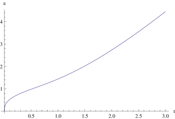
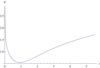
Figure 1: Qualitative behavior of the scale factor (left) and scalar field (right) versus time.

5 Summary

In this letter, we have studied a scalar-vector field model of cosmology in a Noether symmetry point of view, in such a way that in its action, in addition to a minimally coupling between the scalar field and gravity, there is also a coupling between the scalar and the kinetic energy of the vector field. For the background geometry, we have considered a flat FRW metric and then set up the phase space by taking the scale factor $a$, scalar field $\phi$ and the vector field $A$ as the independent dynamical variables. The Lagrangian of the model in the configuration space spanned by $\{a,\phi,A\}$ is so constructed that its variation with respect to these dynamical variables yields the Einstein field equations. The existence of Noether symmetry implies that the Lie derivative of this Lagrangian with respect to the infinitesimal generator of the desired symmetry vanishes. By applying this condition to the Lagrangian of the model, we have obtained the explicit form of the corresponding potential function of the scalar field and the coupling function between the scalar and the vector fields. We then obtained the constant of motion related to the Noether symmetry by means of which we could integrate the dynamics to yield the exact expressions for the dynamical variables $a(t)$, $\phi(t)$ and $A(t)$. The evolutionary behavior of these quantities shows that with a growing vector field we have an isotropic accelerated expansion universe. Our analysis showed that in the early times of evolution the amount of the scalar field decreases continuously to reach a minimum value, simultaneously the kinetic energy of the vector field and its coupling to the scalar field increase. On the other hand, after this period this behavior is reversed, the scalar field begins to increase while its coupling with vector field as well as the vector field’s kinetic energy rapidly decrease. Therefore, in the late times, the universe is scalar field dominated and the vector field plays a subdued role in the expansion in this epoch.

References

• [1] V. I. Arnold, Mathematical Methods of Classical Mechanics (1989) (Springer-Verlag: New York)
• [2] S. Capozziello, G. Marmo, C. Rubano, and P. Scudellaro, Int. J. Mod. Phys. D 06 (1997) (arXiv: gr-qc/9606050) 491
S. Capozziello and G. Lambiase, Gen. Rel. Grav. 32 (2000) 673 (arXiv: gr-qc/9912083)
• [3] S. Capozziello, M. De Laurentis, S.D. Odintsov, Noether Symmetry Approach in Gauss-Bonnet Cosmology (arXiv: 1406.5652 [gr-qc])
A. Paliathanasis, M. Tsamparlis, S. Basilakos, S. Capozziello, (arXiv: 1403.0332 [astro-ph.CO])
T. Christodoulakis, N. Dimakis, Petros A. Terzis, B. Vakili, E. Melas and Th. Grammenos, Phys. Rev. D 89 (2014) 044031 (arXiv: 1309.6106 [gr-qc])
T. Christodoulakis, N. Dimakis, Petros A. Terzis, G. Doulis, Th. Grammenos, E. Melas and A. Spanou, J. Geom. Phys. 71 (2013) 127 (arXiv: 1208.0462 [gr-qc])
B. Vakili and F. Khazaie, Class. Quantum Grav. 29 (2012) 035015 (arXiv: 1109.3352 [gr-qc])
B. Bakili, Int. J. Theor. Phys. 51 (2012) 133 (arXiv: 1102.1682[gr-qc])
S. Capozziello and A. De Felice, J. Cosmol. Astropart. Phys. JCAP08 (2008) 016 (arXiv:0804.2163 [gr-qc])
B. Vakili, Phys. Lett. B 664 (2008) 16 (arXiv: 0804.3449 [gr-qc])
F. Darabi, K. Atazadeh, A. Rezaei-Aghdam, Eur. Phys. J. C 73 (2013) 2657 ( arXiv: 1304.2926 [qr-qc])
A. Paliathanasis, S. Basilakos, E.N. Saridakis, S. Capozziello, K. Atazadeh, F. Darabi and M. Tsamparlis, Phys. Rev. D 89 (2014) 104042 (arXiv: 1402.5935 [gr-qc])
S. Capozziello, M. De Laurentis and S.D. Odintsov, Eur. Phys. J. C 72 (2012) 2068 (arXiv: 1206.4842 [gr-qc])
A. Paliathanasis and M. Tsamparlis, Int. J. Geom. Methods Mod. Phys. 11 (2014) 1450037 (arXiv: 1312.3942 [math-ph])
• [4] J.J. Halliwell, Introductory Lectures on Quantum Cosmology (arXiv: 0909.2566 [gr-qc])
• [5] C. Brans and R.H. Dicke, Phys. Rev. 124 (1961) 925
A.G. Riess et al, Astron. J. 116 (1998) 1009
D.H. Lyth and A. Riotto, Phys. Rep. 314 (1999) 1
T. Padmanabhan, Phys. Rep. 380 (2003) 235
• [6] A. Tartaglia and N. Radicella, Phys. Rev. D 76 (2007) 083501 (arXiv: 0708.0675 [gr-qc])
M. Artymowski and Z. Lalak, J. Cosmol. Astropart. Phys. JCAP09 (2011) 017 (arXiv: 1012.2776 [gr-qc])
S.D. Sadatian, Int. J. Mod. Phys. D 21 (2012) 1250063 (arXiv: 1206.2438 [gr-qc])
O. Akarsu, T. Dereli and N. Oflaz, Class. Quantum Grav. 31 (2014) 045020 (arXiv: 1311.2573 [gr-qc])
• [7] A. Maleknejad, M.M. Sheikh-Jabbari and J. Soda, Gauge Fields and Inflation (arXiv: 1212.2921 [hep-th])