Bogoliubov Theory of Dipolar Bose Gas in Weak Random Potential
Abstract
We consider a dilute homogeneous Bose gas with both an isotropic short-range contact interaction and an anisotropic long-range dipole-dipole interaction in a weak random potential at low temperature in three dimensions. Within the realm of Bogoliubov theory we analyze how both condensate and superfluid are depleted due to quantum and thermal fluctuations as well as disorder fluctuations.
pacs:
03.75.Hh, 67.85.DeI Introduction
Since the first observation of Bose-Einstein condensation (BEC) in 1995 for alkali atomic vapors of 87Rb and 23Na atoms both theoretical and experimental research has accelerated to study this newly discovered macroscopic quantum phenomenon, where a fraction of these bosons occupies the same quantum mechanical ground state. Achieving BEC in experiment for alkali atoms was only possible due to the discovery of efficient cooling and trapping techniques which became available by the end of the twentieth century key-3 ; key-1 ; key-2 . With more cooling advances, research interest has not only increased in the field of ultra-cold quantum gases with isotropic short-range contact interaction, which represents the effective interaction between atoms and is dominated by the s-wave scattering length. Also the anisotropic long-range dipole-dipole interaction has been made accessible to detailed study by the formation of a BEC in a dipolar quantum gas of 52Cr atoms pfau ; pfau-3 . Further atomic BECs with magnetic dipole-dipole interaction followed soon with 164Dy lev and 168Er grimm atoms. Strong electric dipole-dipole interactions were realized by a stimulated Raman adiabatic passage (STIRAP) experiment, which allowed the creation of 40K 87Rb molecules in the rovibrational ground state ospelkhaus ; ospelkhaus1 .
The research field of ultra-cold quantum gases allows today to analyze many condensed matter problems in the spirit of Feynman’s quantum simulator Fenman , as all ingredients of the quantum many-body Hamiltonian can be experimentally tuned with an unprecedented precision. The kinetic energy can be controlled with spin-orbit coupling kinetic ; kinetic1 , the potential energy can be harmonic harmonic box-like hadzib or even anharmonic aharmonic and also the strength of contact as well as dipolar interaction are tunable feshbach ; pfau-1 ; pfau-2 . In addition, in order to make quantum gas simulators even more realistic, various experimental and theoretical methods for controlling the effect of disorder have been designed. Using superfluid helium in vycor glass, which represents some kind of porous media, the random distribution of pores represents a random environment key-4 . Laser speckles are produced by focusing the laser beam on a glass plate, where the resulting random interference pattern is reflected to a BEC cell key-5 ; key-7 ; key-6 ; aspect . Wire traps represent magnetic traps on atomic chips where the roughness and the imperfection of the wire surface generates a disorder potential key-8 ; key-9 . Another possibility to create a random potential is to trap one species of atoms randomly in a deep optical lattice, which serves as frozen scatterers for a second atomic species key-10 ; Schneble . In addition also, incommensurable lattices provide a useful random environment incommen1 ; incommen2 ; incommen3 .
In order to study the properties of interacting bosons in such a random potential Huang and Meng proposed a Bogoliubov theory, which was applied to the case of superfluid helium in porous media key-11 , and extended later by others giorgini ; lopatin ; key-12 ; graham1 . For a delta-correlated disorder it was found that both a condensate and a superfluid depletion occurs due to the localization of bosons in the respective minima of the external random potential which is present even at zero temperature. A generalization to the corresponding situation, where the disorder correlation function falls off with a characteristic correlation length as, for instance, a Gauss function key-14 ; pelster1 , laser speckles pelster2 or a Lorentzian pelster3 is straightforward.
In this paper we extend the Bogoliubov theory of Huang and Meng key-11 to a dipolar Bose gas at finite temperature. With this we go beyond the zero-temperature mean-field approach where the Gross-Pitaevskii equation is solved perturbativly with respect to the random potential pelster1 ; pelster3 . This extension to the finite-temperature regime allows us to study in detail how the anisotropy of superfluidity can be tuned, a phenomenon which also occurs at zero-temperature pelster1 ; pelster3 , but turns out to be enhanced by the thermal fluctuations. We observe in addition that contact and dipolar interaction have different effects upon quantum, thermal, and disorder depletion of condensate and superfluid.
The paper is organized as follows. In Section. II we revisit the Bogoliubov theory of the homogeneous dirty boson problem. With this, we determine for a general two-particle interaction and a general disorder correlation for different observables the beyond mean-field corrections which stem from quantum, thermal, and disorder fluctuations. In Section. III we specialize our treatment for a dipolar Bose gas and a delta-correlated disorder in the zero-temperature and the thermodynamic limit. In particular, we investigate the particle and condensate density as well as the inner energy. In Section. IV we extend the Bogoliubov theory in order to derive the superfluid depletion which turns out to be only due to the external random potential and the thermal excitation. In Section. V we consider how finite-temperature effects on the condensate depletion as well as the normal fluid component depend on the respective strength of contact and dipolar interaction.
II Bogoliubov Theory
A three-dimensional ultra-cold dipolar Bose gas in a weak random potential is modeled by the grand-canonical Hamiltonian
| (1) | ||||
where and are the usual field operators for Bose particles of mass , which satisfy the following commutation relations
| (2) |
Here denotes the chemical potential and represents the random potential. Irrespective of the physical origin of the disorder potential, we assume that the average over the random potential vanishes and that it has some kind of correlation i.e. and . Furthermore, the two-particle interaction potential for a dipolar Bose gas consists of two different parts: . On the one hand the short-range isotropic contact interaction is given by , where represents its strength with the s-wave scattering length . From now on we assume a positive , i.e. a repulsive contact interaction, which depletes the particles from the ground state due to quantum and thermal fluctuations and also forbids them from being localized in the minima of the external random potential . Thus, unlike the case of free fermions, where Pauli blocking prevents the particles from localizing in a single orbital, bosons require a repulsive interaction to prevent them from collapsing into the respective minima of the external random potential. On the other hand the long-range anisotropic polarized dipolar part is written in real space for dipoles aligned along -axis direction according to
| , | (3) |
where represents the dipolar interaction strength due to magnetic or electric dipole moments. In the first case we have , with the magnetic dipole moment and the magnetic permeability of vacuum , and in the latter case we have , with the electric dipole moment and the vacuum dielectric constant . Note that, due to the anisotropic character of the dipolar interaction, many static and dynamic properties of a dipolar Bose gas become tunable pfau ; pfau-3 ; glaum ; glaum1 , consequences for a random environment have only recently be explored pelster1 ; pelster3 .
With the help of a Fourier transformation we can rewrite the Hamiltonian (1) in momentum space according to
| (4) |
where denotes the volume and the interaction potential in momentum space is given by pfau-1
| (5) |
Here denotes the angle between the polarization direction, which is here along the -axis, and the wave vector . Note that (5) is not continuous at , as the limit is direction dependent. This is the origin for various anisotropic properties, which are characteristic for dipolar Bose gases pelster1 ; pelster3 ; key-15 ; lima . The operators and are the annihilation and creation operators in Fourier space, respectively, which turn out to satisfy the bosonic commutation relations
| . | (6) |
Near absolute zero temperature the number of the particles in the ground state becomes macroscopically large. In this case we have due to (6) and , so the operators and approximately commute with each other. Thus we can apply the Bogoliubov prescription bogoliubov and replace the creation and annihilation operators of the ground state by a c-number, i.e. . As a consequence, we have to decompose the respective momentum summations in the Hamiltonian (4) into their ground state and excited states contributions. By doing so, we perform the following two physical approximations. At first, we ignore terms which contain creation and annihilation operators of the excited states , which are of third and fourth order, as they represent higher-order interactions of the particles out of the condensate. Such an approximation is justified in the case of weakly interacting systems. Secondly, we assume for weak enough disorder that disorder fluctuations decouple in lowest order. Therefore, we ignore the terms with both and . Note that these two physical approximations imply that the excited states are only rarely occupied, i.e. . With this we get the simplified Hamiltonian
| (7) |
Here the prime over the summation symbol indicates that the ground state is excluded. The appearance of off-diagonal terms and with in equation (7) indicates that the state is no longer the ground state of the interacting system. In order to determine this new mean-field ground state we have to diagonalize the Hamiltonian (7). To this end we follow Ref. key-11 and use the inhomogeneous Bogoliubov transformation
| (8) |
Note that the Bogoliubov amplitudes and can be chosen to be real without loss of generality. Furthermore, we impose upon the new operators that they also satisfy bosonic commutation relations
| . | (9) |
Inserting (8) in the simplified Hamiltonian (7) we obtain via diagonalization the following results for the Bogoliubov parameters
| (10) |
and the translations
| (11) |
Here we have introduced for brevity the condensate density and the quasi-particle dispersion
| . | (12) |
Note that the diagonalized Hamiltonian changes with each realization of the disorder potential . Therefore, we get the final Hamiltonian of the dirty dipolar Bose system by performing the disorder ensemble average
| (13) |
With this it is straightforward to determine the corresponding grand-canonical potential , where denotes the grand-canonical partition function and is the reciprocal temperature:
| (14) |
Extremizing equation (14) with respect to the condensate density for fixed chemical potential we find up to first order in quantum, thermal, and disorder fluctuations
| (15) | ||||
where the quasi-particle dispersion (12) now reads
| . | (16) |
Note that the zeroth order in (15) represents the mean-field result and corresponds to the Hugenholtz-Pines relation pines . It makes the quasi-particle dispersion (12) according to (16) linear and gapless (massless) in the long-wavelength limit , in accordance with the Nambu-Goldstone theorem nambu ; goldstone .
Inserting (15) in (14) the grand-canonical potential reduces up to first order in all fluctuations to the grand-canonical free energy
| (17) |
The particle number density follows then from equation (17) via the thermodynamic relation :
| (18) |
Eliminating from (15) and (18) the chemical potential allows to determine the condensate depletion up to first order in the respective fluctuations:
| (19) |
Thus the total particle density consists of four parts. Within the Bogoliubov theory the main contribution is due to the condensate density , whereas the occupation of the excited states above the ground state consists of three distinct terms: the condensate depletion due to interaction and quantum fluctuations is denoted by yang
| (20) |
Note that we neglected here any impact of the external random potential upon the quantum fluctuations, an interesting case which was only recently studied in detail in Refs. muller ; muller1 .
The condensate depletion due to the thermal fluctuations is given by
| (21) |
And finally, the condensate depletion due to the external random potential results in
| (22) |
Note that the validity of our approximation depends on the condition , i.e. the depletion is small, so that condensate density and total density are approximately the same. With this dispersion (16) in all fluctuation terms (20)–(22) reduces to
| , | (23) |
which represents the celebrated Bogoliubov spectrum for the collective excitations. Note that in the Popov approximation the particle density in (23) is substituted by the condensate density , so that this Bogoliubov dispersion acquires fluctuation corrections jandersen .
The grand-canonical ground-state energy follows directly from equation (17), by using the thermodynamic relation :
| . | (24) |
The first term on the right-hand side of (24) represents the ground-state mean-field energy for the homogeneous Bose-Einstein condensate, whereas the other three terms denote energy contributions which are due to the partial occupation of the excited states. The energy shift due to interaction and quantum fluctuations is denoted by
| . | (25) |
The energy shift due to the thermal fluctuations is given by
| . | (26) |
And, finally, the energy shift due to the external random potential reads
| . | (27) |
Within the next section these general results are further evaluated and discussed for a dipolar Bose gas.
III Zero-Temperature results
In this section we specialize our results to the zero-temperature limit for a delta-correlated random potential , where denotes the disorder strength. In the thermodynamic limit, when both the particle number and the volume diverge, i.e. and , but their ratio remains constant, the respective wave vector sums converge towards integrals: . With this we obtain for the quantum depletion (20) the concrete result key-15 ; lima
| , | (28) |
with the original Bogoliubov expression bogoliubov
| , | (29) |
whereas the disorder depletion (22) specializes to pelster1 ; pelster3
| . | (30) |
Here denotes the relative dipolar interaction strength, and
| , | (31) |
represents the Huang-Meng result for the isotropic contact interaction key-11 . In addition, the functions
| , | (32) |
which describe the dipolar effect, can be expressed analytically gradshtien
| (33) |
in terms of the hypergeometric function . The dipolar function is depicted in Fig. 1, and increases for increasing magnitude of for both positive and negative sign. Note that, in order to avoid any instability, we restricted in Fig. 1 to the maximum value one, so that the radicand in the Bogoliubov spectrum (23) remains positive when key-15 ; lima .
We conclude that Eqs. (28), (30) reproduce the contact interaction results Eqs. (29), (31) for due to the property . Note that increasing the repulsive contact interaction has opposite effects on the zero-temperature condensate depletion. On the one hand more and more bosons are then scattered from the ground state to some excited states so that the quantum depletion (29) increases. On the other hand the localization of bosons in the respective minima of the random potential is hampered, so that disorder depletion (31) decreases. In contrast to that the long-range dipolar interaction turns out to enhance both the quantum deletion (28) and the disorder depletion (30), see Fig. 1. As the dipolar interaction potential (3) has two repulsive and only one attractive direction in real space, it yields a net expulsion of bosons from the ground state which is described by in (28). In contrast to that the dipolar interaction supports the localization of bosons in the random environment pelster1 ; pelster3 according to in (30). This is due to the fact that the BEC droplets in the respective minima of the random potential can minimize their energy by deformation along the polarization axis pfau-3 . The dipolar enhancement in both the quantum depletion and the external random potential depletion are approximately the same with respect to up to , but then the dipolar enhancement in starts to increase faster than in , see Fig. 1.
Furthermore, we read off from (25) that the energy shift due to the interaction and the quantum fluctuations are ultraviolet divergent. Thus, following Refs. lima ; fetter , we can evaluate (25) by introducing an ultraviolet cutoff, where the interaction has to be renormalized by inserting the term , so that the divergent part is removed
| , | (34) |
evaluations in the thermodynamic limit yielding
| . | (35) |
Another method for (25) relies on Schwinger trick kleinert which leads again to (35). The energy shift due to the external random potential (27) is also ultraviolet divergent:
| . | (36) |
Thus, it is calculated either with an ultraviolet cutoff by subtracting the divergent term , or with the help of the Schwinger trick, leading to
| (37) |
Note that energy shift due to interaction and quantum fluctuations in equation (35) and the external random potential energy shift in equation (37) reproduce the well-known contact interaction results when , and that increases quicker than with respect to . Finally note that both energy shifts (35) and (37) could be used to study the collective properties of a trapped dipolar Bose gas within the local density approximation huang ; huang1 .
IV Superfluidity
Now we extend the Bogoliubov theory in order to study the transport phenomenon of superfluidity within the framework of linear response theory. With this we calculate the superfluid depletions due to both the external random potential and the thermal fluctuations.
IV.1 Bogoliubov theory revisited
Following Refs. key-12 ; ueda we calculate the superfluid component of the Bose gas, which moves with the superfluid velocity , via a linear response approach. To this end we perform a Galilean boost for our system with a boost velocity so that the normal fluid component is dragged along this boost. Inserting the Galilean transformations , , and rewriting the field operator in Heisenberg picture according to , the Hamiltonian in momentum space reads instead of (4)
| (38) |
with the effective chemical potential . Applying the Bogoliubov theory along similar lines as in Section II and after performing the disorder ensemble average of the grand-canonical Hamiltonian we obtain instead of (13)
| (39) |
where stands for the quasi-particle dispersion (12) with substituted by . Now it is straightforward to find the corresponding grand-canonical effective potential, where we get instead of (14):
| (40) |
Within a linear response approach we are only interested in small velocities and , so we expand Eq. (40) up to second order in , and we get
| (41) | ||||
Note that the terms linear in vanish due to symmetry reasons. Extremizing the grand-canonical effective potential (41) with respect the the condensate density yields in zeroth order the mean-field result . With this we are ready to determine the momentum of the system in the small-velocity limit, which turns out to be of the following form
| , | (42) |
where the total density decomposes into the superfluid and normal component and , respectively, and denotes the normal fluid velocity. The normal fluid density turns out to decompose according to , where the contribution due to the external random potential, which only exists in the zero temperature limit, reads pelster1
| , | (43) |
while the normal fluid density due to the thermal fluctuations is given by
| , | (44) |
where stands for the Bogoliubov energy spectrum (23). Note that there is no superfluid depletion in (42) which is due to quantum fluctuations, in contrast to the condensate depletion which has a quantum fluctuations component determined by Eq. (20).
IV.2 Zero-temperature superfluid depletion
Again we specialize at first to the zero-temperature limit and to a delta-correlated random potential and evaluate the corresponding superfluid depletions in the thermodynamic limit. Depending on the boost direction, we have two different superfluid depletions in the directions parallel or perpendicular to the dipole polarization. In the first case the superfluid depletion reads
| , | (45) |
whereas in the second case the superfluid depletion turns out to be
| . | (46) |
Here we have introduced the new function
| , | (47) |
which can also be expressed analytically with the help of the integral table gradshtien according to
| . | (48) |
Note that the function shown in Fig. 2 has the property and decreases slowly with increasing for , while it behaves non-monotonically with increasing for .
We observe that, due to and , both depletions and coincide for vanishing dipolar interaction and equate , which reproduces the Huang-Meng result for the isotropic contact interaction key-11 . Due to the localization of bosons in the respective minima of the random potential the superfluid is hampered, so that the superfluid depletion is larger than the condensate depletion. Switching on the dipolar interaction has a significant effect on both depletions and . Their ratio with the condensate depletion turns out to be monotonically decreasing/increasing with respect to the relative dipolar interaction strength according to Fig. 3. This is explained qualitatively by considering the dipolar interaction in Fourier space (5) as an effective contact interaction pelster1 ; pelster3 . Therefore, for sufficiently large values of , it turns out that becomes even smaller than the condensate depletion. This surprising finding suggests that the localization of the bosons in the minima of the random potential only occurs for a finite period of time graham . As a consequence the ratio decreases monotonically for increasing values of the relative dipolar interaction strength .

V Finite-temperature effects
In the previous sections we restricted the application of the Bogoliubov theory of dirty bosons to the zero-temperature limit. Nevertheless any experiment is performed at finite-temperature, where thermal fluctuations play an important role besides quantum and disorder fluctuations. Therefore, we calculate in this section for a dipolar BEC the contributions to both the condensate and the normal fluid component which are due to thermal excitations.
V.1 Condensate depletion
At zero temperature the condensate depletion consists of two contributions, one due to the quantum fluctuation (20) and another one due to the disorder potential (22), which are evaluated in (28), (30) for a dipolar BEC, respectively. But for increasing temperature also the third contribution (21) of the depletion (19) will play an important role and should be taken into account. This additional term represents the condensate depletion due to the thermal excitations, which reads in the thermodynamics limit
| , | (49) |
where denotes the Bogoliubov spectrum (23). The integral (49) can be recast in dimensionless form
| , | (50) |
where we have introduced the gas parameter , and the relative temperature , with being the critical temperature for the non-interacting Bose gas, and denotes the Riemann zeta function with the value . The remaining integral reads
| , | (51) |
with the abbreviations and . Fig. 4 shows how the condensate thermal fractional depletion (50) increases with the relative temperature for different values of the relative dipolar interaction strength and the gas parameter . For increasing contact interaction, it turns out that decreases as collisions between the thermal particles yield partially a scattering into the macroscopic ground state. In contrast to that we observe that the dipolar interaction has the opposite effect: increasing enhances the thermal depletion . This can be understood from considering the consequences of the dipolar interaction as an effective contact interaction pelster1 ; pelster3 , yielding two attractive and one repulsive direction in Fourier space according to (5).
In order to investigate this qualitative finding more quantitatively in the vicinity of zero temperature but far below the critical temperature, we approximate the condensate depletion (50) analytically like
| (52) |
This reproduces the isotropic contact interaction case for vanishing dipolar interaction due to landau-1 . Note that (52) turns out to approximate (51) quite well irrespective of and in the temperature range . Here also each term in (52) decreases for increasing , while it is enhanced for increasing .
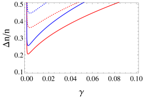
Now we investigate how the validity range of the Bogoliubov theory depends on the gas parameter and the relative temperature for different values of the relative dipolar interaction strength and the disorder strength . To this end we restrict the condensate depletion in equation (19) to be limited maximally by half of the particle number density . Inserting the critical temperature for the non-interacting Bose gas and the gas parameter in the condensate depletion due to quantum fluctuation (28) and random potential (30), the fractional depletion reads

| (53) |
Here the thermal fractional condensate depletion (50) in (53) is determined numerically from (51) and from (52) analytically in the vicinity of zero temperature for comparison. Fig. 5 depicts the resulting validity range of the Bogoliubov theory in the clean case i.e. the disorder strength , and in the dirty case with . It is represented by the area below the curves when the condensate depletion is equal to . Outside this area the Bogoliubov approximation is not valid. Note that the validity range (50), (53) is well approximated by (52) near zero temperature. From (50), (53) we read off that the Bogoliubov theory is not applicable near the critical temperature. Furthermore the validity range decreases for increasing values of the relative dipolar interaction strength , and it also smaller in the dirty case compared to the clean one.
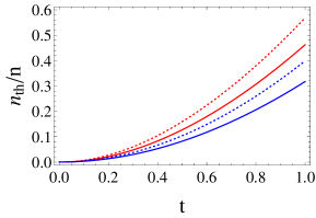
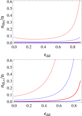
Finally, we plot in Fig. 6 the total fractional condensate depletion versus the gas parameter with the thermal fractional condensate depletion in (53) inserted from (50) for the disorder strength . Note that the sharp increase for small gas parameter is unphysical due to the fact that the Bogoliubov theory is no longer valid, see Fig. 5. We conclude that increasing the parameters and yields an increasing fractional depletion.

V.2 Superfluid depletion
Now we calculate the superfluid depletion for the dipolar Bose gas which is due to thermal fluctuations. In the thermodynamic limit of equation (44) the components parallel and perpendicular to the dipole polarization direction have to be evaluated separately. Parallel to the dipoles the integral reads in dimensionless form
| , | (54) |
where the remaining integral is written explicitly as
| . | (55) |
In the direction perpendicular to the dipoles the superfluid depletion reads in dimensionless form
| , | (56) |
where the remaining integral is written explicitly as
| . | (57) |
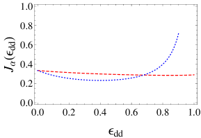
Fig. 7 shows how the superfluid thermal fractional depletions parallel and perpendicular to the polarized dipoles depend on the respective values of the parameters , , and . The perpendicular superfluid depletion behaves similar to the condensate thermal depletion , i.e. is enhanced for increasing and , whereas it is reduced for increasing . Also for we observe that it depends on and , like and , i.e. it increases with but decreases with . But, surprisingly, it turns out that has a nontrivial dependence on , where we have first a decrease and then an increase for increasing . Fig. 8 highlights in more detail how the superfluid thermal fractional depletions changes versus relative dipolar interaction strength .
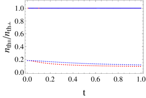
Note that both and coincide for vanishing dipolar interaction as follows from Fig. 9 which shows the thermal superfluid depletion ratio versus the relative temperature . When the dipolar interaction is present we notice that the ratio reveals only a tiny - and -dependence which is decreasing with and increasing with , respectively. In Fig. 10 we plot the thermal superfluid depletions ratio versus the relative dipolar strength . It shows that both and coincide for vanishing dipolar interaction, and the ratio decreases for increasing values of the relative dipolar strength .

In the vicinity of the zero temperature but far below critical temperature we can approximate the superfluid depletion in (54) analytically. We find that the superfluid depletion parallel to the dipoles reads
| . | (58) |
which has a non-monotonic behavior versus due to the function , which is plotted in Fig. 2 where we have a decrease at first and then an increase for increasing . Furthermore, the superfluid depletion perpendicular to the dipoles reads
| . | (59) |
so that is enhanced for increasing due to the fact that the function shown in Fig. 1 increases faster than the function shown in Fig. 2. A comparison between the two different superfluid depletions shows that both and coincide for vanishing dipolar interaction, and reproduce the isotropic contact interaction result landau-1 due to and . The ratio from (58), (59) decreases for increasing values of the relative dipolar strength as is shown in gray color in Fig. 10


V.3 Superfluid Ratios
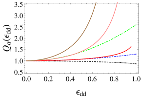
Finally after having discussed the different origins of the superfluid depletions for the dipolar Bose gas, we discuss now the ratios of the total superfluid depletions over the total condensate depletion for different values of the respective parameters , , and . We consider both the clean case where the disorder strength and in the dirty case with . Fig. 11 shows the clean case with the ratios (upper) and (lower) versus relative dipolar strength . For increasing and , both and are enhanced, but increasing decreases both and .
Fig. 12 shows in the dirty case the ratios (upper) and (lower) versus relative dipolar strength . For increasing we will get enhancement for , regardless of the temperature , while for we will get enhancement for small values of and then upon increasing , we observe a decrease up to and then an increase, which shows that the disorder changes the situation a lot compared to the clean case in Fig. 11. Increasing will cause a more complex interplay on both and , as is seen in Fig. 12.
VI Conclusion
In this paper we have investigated the dipolar dirty boson problem,
where both the short-range isotropic contact interaction as well as
the anisotropic long-range dipole-dipole interaction are present within
a Bogoliubov theory at low temperatures below the critical temperature.
In the zero-temperature limit, we discussed analytically the nontrivial
results for both the condensate and the superfluid depletions as well as
the interplay between the long-range anisotropic dipolar interaction
and the external random potential which yields an anisotropic superfluidity
pelster1 ; pelster3 . At finite temperature, we obtained, due
to the long-range anisotropic dipole-dipole interaction, different
analytical and numerical results for condensate and the superfluid
depletions, where the latter depends sensitively on whether the flow
direction is parallel or perpendicular to the dipolar polarization
axis. It still remains to investigate how the Josephson relation between condensate and superfluid densities reads
for a disordered dipolar superfluid cord .
VII Acknowledgment
We both acknowledge fruitful discussions with T. Checinski and A. R. P. Lima. M. Ghabour thanks his family for financial support during this work. A. Pelster thanks for the support from the German Research Foundation (DFG) via the Collaborative Research Center SFB /TR49 Condensed Matter Systems with Variable Many-Body Interactions.
References
- (1) J. Stenger, D. M. Stamper-Kurn, M. R. Andrews, A. P. Chikkatur, S. Inouye, H. J. Miesner, and W. Ketterle. J. Low Temp. Phys. 113, 167 (1998).
- (2) F. Dalfovo, S. Giorgini, L. P. Pitaevskii, and Sandro Stringari. Rev. Mod. Phys. 71, 463 (1999).
- (3) A. J. Leggett. Rev. Mod. Phys. 73, 307 (2001).
- (4) A. Griesmaier, J. Werner, S. Hensler, J. Stuhler, and T. Pfau. Phys. Rev. Lett. 94, 160401 (2005).
- (5) T. Lahaye, T. Koch, B. Frohlich, M. Fattori, J. Metz, A. Griesmaier, S. Giovanazzi, and T. Pfau. Nature 448, 672 (2007).
- (6) M. Lu, N. Q. Burdick, S. H. Youn, and B. L. Lev. Phys. Rev. Lett. 107, 190401 (2011).
- (7) K. Aikawa, A. Frisch, M. Mark, S. Baier, A. Rietzler, R. Grimm, and F. Ferlaino. Phys. Rev. Lett. 108, 210401 (2012).
- (8) S. Ospelkaus, K. K. Ni, M. H. G. de Miranda, B. Neyenhuis, D. Wang, S. Kotochigova, P. S. Julienne, D. S. Jin, and J. Ye. Faraday Discuss. 142, 351 (2009).
- (9) S. Ospelkaus, K. K. Ni, G. Quèmèner, B. Neyenhuis, D. Wang, M. H. G. de Miranda, J. L. Bohn, J. Ye, and D. S. Jin. Phys. Rev. Lett. 104, 030402 (2010).
- (10) R. Feynman. Int. J. Theo. Phys. 21, 467 (1982).
- (11) Y. J. Lin, R. L. Compton, K. Jiménez-García, J. V. Porto, and I. B. Spielman. Nature 462, 628 (2009).
- (12) Y. J. Lin, K. Jiménez-García, and I. B. Spielman. Nature 471, 83 (2011).
- (13) H. J. Metcalf and P. van der Straten, Laser Cooling and Trapping (Springer, Berlin, 1999).
- (14) A. L. Gaunt, T. F. Schmidutz, I. Gotlibovych, R. P. Smith, and Z. Hadzibabic. Phys. Rev. Lett. 110, 200406 (2013).
- (15) V. Bretin, S. Stock, Y. Seurin, and Jean Dalibard. Phys. Rev. Lett. 92, 050403 (2004).
- (16) S. Inouye, M. R. Andrews, J. Stenger, H. J. Miesner, D. M. Stamper-Kurn, and W. Ketterle. Nature 392, 151 (1998).
- (17) K. Góral, K. Rzaźewski, and T. Pfau. Phys. Rev. A 61, 051601(R) (2000).
- (18) S. Giovanazzi, A. Görlitz and T. Pfau. Phys. Rev. Lett. 89, 130401 (2002).
- (19) B. C. Crooker, B. Hebral, E. N. Smith, Y. Takano, and J. D. Reppy. Phys. Rev. Lett. 51, 666 (1983).
- (20) J. E. Lye, L. Fallani, M. Modugno, D. S. Wiersma, C. Fort, and M. Inguscio. Phys. Rev. Lett. 95, 070401 (2005).
- (21) D. Clement, A. F. Varon, J. A. Retter, L. Sanchez-Palencia, A. Aspect, and P. Bouyer. New J. Phys. 8, 165 (2006).
- (22) L. Sanchez-Palencia, D. Clement, P. Lugan, P. Bouyer, and A. Aspect. New J. Phys. 10, 045019 (2008).
- (23) J. Billy, V. Josse, Z. Zuo, A. Bernard, B. Hambrecht, P. Lugan, D. Clement, L. Sanchez-Palencia, P. Bouyer, and A. Aspect. Nature 453, 891 (2008).
- (24) P. Krüger, L. M. Andersson, S. Wildermuth, S. Hofferberth, E. Haller, S. Aigner, S. Groth, I. Bar-Joseph, and J. Schmiedmayer. Phys. Rev. A 76, 063621 (2007).
- (25) J. Fórtagh and C. Zimmermann. Rev. Mod. Phys. 79, 235 (2007).
- (26) U. Gavish and Y. Castin. Phys. Rev. Lett. 95, 020401 (2005).
- (27) B. Gadway, D. Pertot, J. Reeves, M. Vogt, and D. Schneble. Phys. Rev. Lett. 107, 145306 (2011).
- (28) B. Damski, J. Zakrzewski, L. Santos, P. Zoller, and M. Lewenstein. Phys. Rev. Lett. 91, 080403 (2003).
- (29) T. Schulte, S. Drenkelforth, J. Kruse, W. Ertmer, J. Arlt, K. Sacha, J. Zakrzewski, and M. Lewenstein. Phys. Rev. Lett. 95, 170411 (2005).
- (30) G. Roati, C. D’Errico, L. Fallani, M. Fattori, C. Fort, M. Zaccanti, G. Modugno, M. Modugno, and M. Inguscio. Nature 453, 895 (2008).
- (31) K. Huang and H. F. Meng. Phys. Rev. Lett. 69, 644 (1992).
- (32) S. Giorgini, L. Pitaevskii, and S. Stringari. Phys. Rev. B 49, 12938 (1994).
- (33) A. V. Lopatin and V. M. Vinokur. Phys. Rev. Lett. 88, 235503 (2002).
- (34) G. M. Falco, A. Pelster, and R. Graham. Phys. Rev. A 75, 063619 (2007).
- (35) R.Graham and A. Pelster. Functional Integral Approach to Disordered Bosons. World Scientific (2007)
- (36) M. Kobayashi and M. Tsubota. Phys. Rev. B 66, 174516 (2002).
- (37) C. Krumnow and A. Pelster. Phys. Rev. A 84, 021608(R) (2011).
- (38) B. Abdullaev and A. Pelster. Eur. Phys. J. D 66, 314 (2012).
- (39) B. Nikolic, A. Balaz, and A. Pelster. Phys. Rev. A 88, 013624 (2013).
- (40) K. Glaum, A. Pelster, H. Kleinert, and T. Pfau. Phys. Rev. Lett. 98, 080407 (2007).
- (41) K. Glaum and A. Pelster. Phys. Rev. A 76, 023604 (2007).
- (42) A. R. P. Lima and A. Pelster. Phys. Rev. A 84, 041604(R) (2011).
- (43) A. R. P. Lima and A. Pelster. Phys. Rev. A 86, 063609 (2012).
- (44) N. N. Bogoliubov. J. Phys.(USSR) 11, 4 (1947).
- (45) N. M. Hugenholtz, and D. Pines. Phys. Rev. 116, 489 (1959).
- (46) Y. Nambu. Phys. Rev. Lett. 4, 380 (1960).
- (47) J. Goldstone. Nuovo Cim. 19, 154 (1961).
- (48) T. D. Lee, K. Huang, and C. N. Yang. Phys. Rev. 106, 1135 (1957).
- (49) C. Gaul and C. A. Müller. Phys. Rev. A 83, 063629 (2011).
- (50) C. A. Müller and C. Gaul. New J. Phys. 14, 075025 (2012).
- (51) J. O. Andersen. Rev. Mod. Phys. 76, 599 (2004).
- (52) I. S. Gradshteyn and I. M. Ryzhik, Table of Integrals, Series, and Products, 7th ed. (Academic Press, New York, 2007).
- (53) A. L. Fetter and J. D. Walecka, Quantum Theory of Many- Particle Systems, (Dover, New York, 2003).
- (54) H. Kleinert and V. Schulte-Frohlinde, Critical Properties of -Theories, (World Scientific, Singapore, 2001).
- (55) E. Timmermans, P. Tommasini, and K. Huang, Phys. Rev. A 55, 3645 (1997).
- (56) G. M. Falco, A. Pelster, and R. Graham, Phys. Rev. A 76, 013624 (2007).
- (57) M. Ueda, Fundamentals and New Frontiers of Bose-Einstein Condensation (World Scientific, Singapore, 2010).
- (58) R. Graham and A. Pelster. Int. J. Bif. Chaos 19, 2745 (2009).
- (59) E. Lifshitz and L. Pitaevskii, Statistical Physics, Part 2 (Elsevier, Oxford, 2003).
- (60) C. A. Müller. arxiv: 1409.6987.