Quasi-convex Hamilton-Jacobi equations posed on junctions: the multi-dimensional case

Abstract

A multi-dimensional junction is obtained by identifying the boundaries of a finite number of copies of an Euclidian half-space. The main contribution of this article is the construction of a multidimensional vertex test function $G(x,y)$. First, such a function has to be sufficiently regular to be used as a test function in the viscosity solution theory for quasi-convex Hamilton-Jacobi equations posed on a multi-dimensional junction. Second, its gradients have to satisfy appropriate compatibility conditions in order to replace the usual quadratic penalization function $|x-y|^{2}$ in the proof of strong uniqueness (comparison principle) by the celebrated doubling variable technique. This result extends a construction the authors previously achieved in the network setting. In the multi-dimensional setting, the construction is less explicit and more delicate.

Mathematical Subject Classification:

35F21, 49L25, 35B51.

Keywords:

Hamilton-Jacobi equations, multi-dimensional junctions, multi-dimensional vertex test function.

Contents

1. 1 Introduction
2. 2 Important functions related to Hamiltonians
3. 3 Approximate construction in the smooth convex case
4. 4 Proof of the main theorem
5. 5 Flux-limited solutions on a multi-dimensional junction
6. A Relaxed solutions, effective junction conditions and Ishii solutions

1 Introduction

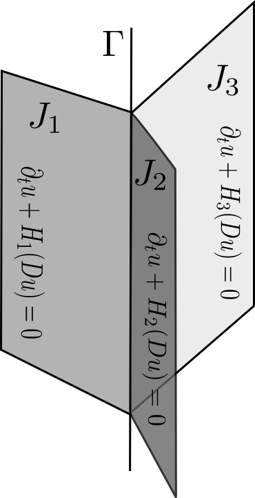
Figure 1: A Hamilton-Jacobi equation posed on a multi-dimensional junction. Here there are 3 branches (or sheets – $N=3$) and the tangential dimension is $1$ ($d=1$). We did not illustrate the junction condition on the junction hyperplane $\Gamma$ (which is a line in this example).

A multi-dimensional junction is made of a finite number of copies of an Euclidian half-space glued through their boundaries (see Figure 1).

$$J=\bigcup_{i=1,...,N}J_{i}\quad\quad\mbox{with}\quad\left\{\begin{array}[]{l}J_{i}=\{X=(x^{\prime},x_{i}):x^{\prime}\in\mathbb{R}^{d},x_{i}\geq 0\}\simeq\mathbb{R}^{d}\times[0,+\infty)\vskip 3.0pt plus 1.0pt minus 1.0pt\\ J_{i}\cap J_{j}=\Gamma\simeq\mathbb{R}^{d}\times\left\{0\right\}\quad\mbox{for}\quad i\not=j\end{array}\right.$$ (1.1)

(with $N\geq 1$ and $d\geq 0$). It was previously considered in [10] and referred to as an open book. It was also considered in [16].

The common boundary $\Gamma$ of the half-spaces $J_{i}$ is referred to as the junction hyperplane. For points $X,Y\in J$, the distance $d(X,Y)$ is defined as follows

$$d^{2}(X,Y)=\begin{cases}|x^{\prime}-y^{\prime}|^{2}+(x+y)^{2}&\text{ if }X\in J_{i},Y\in J_{j},i\neq j\\ |x^{\prime}-y^{\prime}|^{2}+|x-y|^{2}&\text{ if }X,Y\in J_{i}.\end{cases}$$

For a sufficiently regular real-valued function $u$ defined on $J$, $\partial_{i}u(X)$ denotes the (spatial) derivative of $u$ with respect to $x_{i}$ at $X=(x^{\prime},x_{i})\in J_{i}$ and $D^{\prime}u(X)$ denotes the (spatial) gradient of $u$ with respect to $x^{\prime}$. The “gradient” of $u$ is defined as follows,

$$Du(X):=\begin{cases}(D^{\prime}u(X),\partial_{i}u(X))&\quad\mbox{if}\quad X\in J_{i}^{*}:=J_{i}\setminus\Gamma,\\ (D^{\prime}u(x^{\prime},0),\partial_{1}u(x^{\prime},0),...,\partial_{N}u(x^{\prime},0))&\quad\mbox{if}\quad X=(x^{\prime},0)\in\Gamma.\end{cases}$$ (1.2)

With such a notation in hand, we consider a Hamilton-Jacobi equation posed on the multi-dimensional junction $J$ of the form

$$\left\{\begin{array}[]{lll}u_{t}+H_{i}(Du)=0&t>0,X\in J_{i}\setminus\Gamma,\\ u_{t}+F_{A}(Du)=0&t>0,X\in\Gamma\end{array}\right.$$ (1.3)

subject to the initial condition

$$u(0,X)=u_{0}(X)\quad\mbox{for}\quad X\in J.$$ (1.4)

The Hamiltonians satisfy the following assumptions.

$$\left\{\begin{array}[]{ll}\text{\bf(Continuity)}&H_{i}\in C(\mathbb{R}^{d+1})\vskip 6.0pt plus 2.0pt minus 2.0pt\\ \text{\bf(Quasi-convexity)}&\forall\lambda,\{p\in\mathbb{R}^{d+1}:H_{i}(p)\leq\lambda\}\text{ is convex}\vskip 6.0pt plus 2.0pt minus 2.0pt\\ \text{\bf(Coercivity)}&\lim_{|p|\to+\infty}H_{i}(p)=+\infty.\end{array}\right.$$ (1.5)

The real number $\pi_{i}^{0}(p^{\prime})$ is the minimal $\hat{p}_{i}\in\mathbb{R}$ such that $p_{i}\mapsto H_{i}(p^{\prime},p_{i})$ reaches its minimum at $\hat{p}_{i}$. The function $H_{i}^{-}$ is defined by

$$H_{i}^{-}(p^{\prime},p_{i})=\begin{cases}H_{i}(p^{\prime},p_{i})&\quad\mbox{if}\quad p_{i}\leq\pi_{i}^{0}(p^{\prime}),\\ H_{i}(p^{\prime},\pi_{i}^{0}(p^{\prime}))&\quad\mbox{if}\quad p>\pi_{i}^{0}(p^{\prime})\end{cases}$$

(see Figure 2 in Section 2).

The junction function $F_{A}$ appearing in (1.3) is constructed from the Hamiltonians $H_{i}$ and a function $A$ defined on the tangent space of $\Gamma$, referred to as a flux limiter. After identifying the tangent space of $\Gamma$ with $\mathbb{R}^{d}$, flux limiters are functions $A\colon\mathbb{R}^{d}\to\mathbb{R}$ satisfying the following assumption.

$$\left\{\begin{array}[]{ll}\text{\bf(Continuity)}&A\in C(\mathbb{R}^{d})\vskip 6.0pt plus 2.0pt minus 2.0pt\\ \text{\bf(Quasi-convexity)}&\forall\lambda,\{p\in\mathbb{R}^{d}:A(p)\leq\lambda\}\text{ is convex}.\end{array}\right.$$ (1.6)

An example of such a flux limiter is given by

$$A_{0}(p^{\prime})=\max_{i=1,...,N}A_{i}(p^{\prime})\quad\text{ with }\quad A_{i}(p^{\prime})=\min_{p_{i}\in\mathbb{R}}H_{i}(p^{\prime},p_{i}).$$ (1.7)

The function $F_{A}$ is defined as

$$F_{A}(p^{\prime},p_{1},\dots,p_{N})=\max\left(A(p^{\prime}),\max_{i=1,...,N}H_{i}^{-}(p^{\prime},p_{i})\right)$$ (1.8)

(recall the junction condition in (1.3) and the definition of $Du(x)$ in (1.2) for $x\in\Gamma$).

Main result.

Our main result is the existence of the multi-dimensional vertex test function, a “sufficiently” regular function defined on $J^{2}$ whose gradients satisfy appropriate compatibility conditions. In the following statement, $C(J)$ and $C(J^{2})$ denote the classes of continuous functions in $J$ and $J^{2}$ respectively. The class of functions $C^{1}(J)$ is made of functions of $C(J)$ such that the restrictions to $J_{i}$ are $C^{1}$ up to $\Gamma$ – see (1.14) below.

Theorem 1.1 (The vertex test function).

Let $A$ satisfy (1.6) with $A\geq A_{0}$ and let $\gamma\in(0,1]$ be a small error parameter. Assume the Hamiltonians satisfy (1.5). Then there exists a function $G:J^{2}\to\mathbb{R}$ enjoying the following properties.

1. (Regularity)

   $$G\in C(J^{2})\quad\text{and}\quad\left\{\begin{array}[]{l}G(X,\cdot)\in C^{1}(J)\quad\text{for all}\quad X\in J,\\ G(\cdot,Y)\in C^{1}(J)\quad\text{for all}\quad Y\in J.\end{array}\right.$$

2. (Bound from below) $G\geq 0=G(0,0)$.

3. (Compatibility condition on the diagonal) For all $X\in J$,

   $$0\leq G(X,X)-G(0,0)\leq\gamma.$$ (1.9)

4. (Superlinearity) There exists $g:[0,+\infty)\to\mathbb{R}$ nondecreasing and such that for $(X,Y)\in J^{2}$

   $$g(d(X,Y))\leq G(X,Y)\quad\text{and}\quad\lim_{a\to+\infty}\frac{g(a)}{a}=+\infty.$$ (1.10)

5. (Gradient bounds) For all $K>0$, there exists $C_{K}>0$ such that for all $(X,Y)\in J^{2}$,

   $$d(X,Y)\leq K\quad\Longrightarrow\quad|D_{X}G(X,Y)|+|D_{Y}G(X,Y)|\leq C_{K}.$$ (1.11)

6. (Compatibility condition on the gradients) There exists a family of modulus of continuity $\{\omega_{R}\}_{R>0}$ such that for all $X,Y\in J$ and $K>0$ with $d(X,Y)\leq K$,

   $$\left.\begin{array}[]{ll}H_{j}(-D_{Y}G(X,Y))-H_{i}(D_{X}G(X,Y))\leq\omega_{C_{K}}(\gamma C_{K})&\text{ if }Y\in J_{j}^{*},X\in J_{i}^{*}\\ H_{j}(-D_{Y}G(X,Y))-F_{A}(D_{X}G(X,Y))\leq\omega_{C_{K}}(\gamma C_{K})&\text{ if }Y\in J_{j}^{*},X\in\Gamma\\ F_{A}(-D_{Y}G(X,Y))-H_{i}(D_{X}G(X,Y))\leq\omega_{C_{K}}(\gamma C_{K})&\text{ if }Y\in\Gamma,X\in J_{i}^{*}\\ F_{A}(-D_{Y}G(X,Y))-F_{A}(D_{X}G(X,Y))\leq\omega_{C_{K}}(\gamma C_{K})&\text{ if }Y\in\Gamma,X\in\Gamma\end{array}\right\}$$ (1.12)

   with $C_{K}$ given in (1.11).

Remark 1.2.

We recall that for $X\in\Gamma$ (resp. $Y\in\Gamma$), the gradient $D_{X}G(X,Y)$ (resp. $D_{Y}G(X,Y)$) is defined in (1.2).

Theorem 1.1 implies strong uniqueness for (1.3)-(1.4). As a matter of fact, it even implies strong uniqueness for a large class of Hamilton-Jacobi equations posed on a generalized junction, see Remark 1.4 for further details. In order to state the strong uniqueness result for (1.3)-(1.4), we first make precise in which weak sense the solutions satisfy the equation and the junction condition. The appropriate notion is the one of flux-limited solutions [13]: these solutions are viscosity solutions à la Crandall-Evans-Lions satisfying the junction condition in the strong viscosity sense. More precisely, they satisfy the equation in the classical viscosity sense away from the junction hyperplane and they satisfy the junction condition in the viscosity sense with test functions that are continuous in $J$ and $C^{1}$ on each $J_{i}$ up to $\Gamma$ – see Subection 5.1 for a precise definition.

Theorem 1.3 (Comparison principle on a multi-dimensional junction).

Assume that the Hamiltonians $H_{i}$ satisfy (1.5), the flux limiter $A$ satisfies (1.6) with $A\geq A_{0}$ where $A_{0}$ is defined in (1.7), and that the initial datum $u_{0}$ is uniformly continuous. Then for all flux-limited sub-solution $u$ and flux-limited super-solution $v$ of (1.3)-(1.4) satisfying for some $T>0$ and $C_{T}>0$ and $X_{0}\in J$,

$$\begin{cases}u(t,X)\leq C_{T}(1+d(X_{0},X)),\\ v(t,X)\geq-C_{T}(1+d(X_{0},X)),\end{cases}\quad\text{for all}\quad(t,X)\in[0,T)\times J,$$ (1.13)

and such that $u(0,X)\leq u_{0}(X)\leq v(0,X)$ for all $X\in J$, we have $u\leq v\text{ in }[0,T)\times J.$

Remark 1.4.

A comparison principle holds true for Hamilton-Jacobi equations associated with more general junction conditions, see (A.1) and Assumptions (A.3) and (A.4) in Appendix. It is a consequence of the fact that imposing general junction conditions reduce to imposing $F_{A}$ ones, see Theorem A.14 in Appendix. These results extend the ones obtained in the one-dimensional setting [13].

Remark 1.5.

Extensions to Hamiltonians depending on $(t,x)$ is not difficult and is explained in [13] in the network setting. Such an extension is obtained by classically localizing the study around a point $(\bar{t},\bar{x})\in(0,T)\times\Gamma$ at the beginning of the proof of the comparison principle. In the remainder of the proof, one uses the vertex test function associated with the Hamiltonians whose dependence in $(t,x)$ is frozen at $(\bar{t},\bar{x})$, see [13] for details.

Remark 1.6.

This comparison principle holds true for semi-solutions growing at most linearly, see (1.13). Such a condition is classical for such equations.

Difficulties related to strong uniqueness for (1.3).

Getting a strong uniqueness result is known to be difficult for Hamilton-Jacobi equations such as (1.3). Indeed, even the special case $N=2$ is difficult since it corresponds to the study of a Hamilton-Jacobi equation posed in an Euclidian space whose Hamiltonian is discontinuous with respect to the space variable along a hyperplane. More precisely, two different continuous Hamiltonians are chosen on either side of the hyperplane but they do not coincide on it. This discontinuity is identified as a major difficulty when proving a strong uniqueness result such as a comparison principle (Theorem 1.3). It is classically proved by the doubling variable technique: the supremum of $u-v$ in $(0,T)\times J$ is approximated by the supremum of $u(t,x)-v(t,y)-P_{\varepsilon}(x,y)$ in $(0,T)\times J\times J$ where $P_{\varepsilon}(x,y)$ is a penalization function; the behaviour at infinity of the function $P_{\varepsilon}(x,y)$ and the smallness of the parameter $\varepsilon$ force $x$ to be close to $y$. Classically, $P_{\varepsilon}(x,y)$ is chosen as the quadratic function $\varepsilon^{-1}|x-y|^{2}$; but with such a choice, the proof fails because of the discontinuity of the Hamiltonian through the hyperplane. Indeed, two viscosity inequalities are written at points $(\bar{t},\bar{x})$ and $(\bar{t},\bar{y})$ if the approximate supremum is reached at $(\bar{t},\bar{x},\bar{y})$; if $\bar{x}$ and $\bar{y}$ are not in the same $J_{i}$, then the Hamiltonians appearing in the two viscosity inequalities are different. Some authors impose compatibility conditions on Hamiltonians but we do not want to do so. Instead, a natural idea [1, 13] is to design the penalization function $P_{\varepsilon}(x,y)$ in such a way that it compensates the lack of compatibility conditions between Hamiltonians. Here, it is chosen in the form $\varepsilon G(x/\varepsilon,y/\varepsilon)$ for some function $G$ referred to as a vertex test function. The compatibility conditions on the gradients vi) of $G$ in Theorem 1.1 address the lack of compatibility of Hamiltonians.

Apart from the compatibility conditions on the gradients, see vi), other properties of the vertex test function $G$ are needed. The regularity of $G$, see i), allows one to use it as a test function in $X$ and $Y$. The bound from below, see ii), the compatibility on the diagonal, see iii), and the superlinearity, see iv), ensure that $G$ can be used as a penalization function. The gradient bounds, see v), are necessary to handle the unboundedness of the domain.

Difficulties associated with the multidimensional setting.

The construction of the vertex test function is constructed in two steps: first an approximate vertex test function is defined, which satisfies the desired properties except on the set $\{x=y\}$ of $J\times J$; second this approximate vertex test function is regularized on the set $\{x=y\}$. In the multidimensional setting, each step is significantly more difficult than in the one-dimensional setting. When constructing the approximate vertex test function, an optimization problem with equality constraints has to be solved and the optimizer is defined implicitly through first order optimality conditions, while in the one-dimensional setting, this optimization problem is trivial and the optimizer explicit. As far as the second step is concerned, it is much more involved to check that the regularization procedure does not affect the other properties.

Comparison with known results.

In the special case $N=2$, our results are related to [4, 5] where an optimal control problem in a two-domain setting is studied. In these works, the state of the system evolves according to two different dynamics on each side of an hypersurface. Moreover, the two dynamics at the interface corresponding to the maximal and minimal Ishii’s discontinuous solutions of the associated Hamilton-Jacobi equation are identified. One of the two value functions is characterized in terms of partial differential equations. We showed in [13] that, in the one-dimensional setting, both value functions can be conveniently characterized by using the notion of flux-limited solutions introduced in [13]. The result of the present paper indicates that such a connexion holds in the general two-domain setting, even if this is out of the scope of the present paper. Moreover, we can deal with quasi-convex Hamiltonians instead of convex ones.

Achdou, Oudet and Tchou [2] use ideas from [4, 5] to get a simple proof of the comparison principle on a (one-dimensional) junction for stationary equations. Then Oudet [16] extended the results to the multi-dimensional setting, getting a comparison principle for stationary problems. The reader can observe that this strong uniqueness result is very similar to the comparison principle obtained in the present paper; the two works were independent and achieved approximately at the same time. A two-domain Hamilton-Jacobi equation of the form (1.3) also appears naturally in the singular perturbation problem studied in [3].

We would like to mention that the results of [4, 5] were recently extended to the general case of stratified spaces in the very nice paper [7]. Such results also extend the ones from [8]. Some results for discontinuous solutions of Hamilton-Jacobi equations in stratified spaces can be found in [12]. In [9], the authors study eikonal equations in ramified spaces. The reader is also referred to [18, 17] for optimal control problems in multi-domains. In particular, the authors impose some transmission conditions. Up to a certain extent, some of our results are related to the ones in [11], in particular, in the case of source terms located on hyperplanes. We finally refer the reader to the numerous references given in [13] and the comments there.

We mentioned that our main motivation for constructing such a vertex test function is the proof of a comparison principle for Hamilton-Jacobi equations. Two years after the first version of this paper was posted, a simpler and alternative proof of this strong uniqueness result was given in [6]; it is obtained as a combination of the ideas from [4, 5, 13] and the present paper. We also recall that the results of the present paper (see Subsection A.3) are used in [14].

Remark 1.7.

In a first version of this paper, the material was presented in a different way. In order to emphasize the main contribution of the present article, we decided to focus the presentation on the construction of the vertex test function and the proof of the comparison principle for flux-limited solutions and to move into an Appendix results related to relaxed solutions. The reason for doing so is that the proofs of the results in the Appendix are (more or less) a straightforward adaptation from the one-dimensional case. The reader is also referred to [14] where the results in the Appendix are generalized to the case of degenerate parabolic equations. Moreover, the multi-dimensional results of Subsection A.3 are used in [14].

Organization of the article.

The paper is organized as follows. We start with the short Section 2 where important functions related to Hamiltonians are defined. Section 3 is devoted to the construction of an approximate vertex test function in the case where the Hamiltonians are smooth and convex. Then the main theorem, Theorem 1.1, is proved in Section 4. Section 5 contains the definition of flux-limited solutions and the proof of the comparison principle (Theorem 1.3). Appendix A begins with the definition of relaxed solutions for Hamilton-Jacobi equations posed on multidimensional junctions (Subsection A.1). The classification of general junction conditions is explained in Subsection A.2. Subsection A.3 is devoted to the special case $N=2$ where maximal and minimal Ishii solutions are related to flux-limited solutions.

Notation.

The junction hyperplane $\Gamma$ is the common boundary of $J_{i}$: we have $\Gamma=\partial J_{i}$. We identify $\Gamma$ with $\mathbb{R}^{d}$ and we do not write the injection of $\mathbb{R}^{d}$ into $J_{i}$: $x^{\prime}\mapsto(x^{\prime},0)$. For this reason, we write indisctinctively $x=(x^{\prime},0)\in\Gamma$ and $x^{\prime}\in\Gamma$.

We set

$$C^{1}(J)=\left\{\phi\in C(J),\quad\mbox{$\phi$ restricted to $J_{i}$ is $C^{1}$ for $i=1,\dots,N$}\right\}.$$ (1.14)

For a function $f:D\to\mathbb{R}$, $\operatorname{epi}f$ denotes its epigraph $\{(X,r)\in D\times\mathbb{R}\colon r\geq f(X)\}$.

2 Important functions related to Hamiltonians

This short section is devoted to the introduction of important functions that are associated with Hamiltonians $H_{i}$: the “natural” flux limiter $A_{0}$, the monotone parts $H_{i}^{\pm}$, the inverse functions $\pi_{i}^{\pm}$.

The functions $A_{0},A_{1},\dots,A_{N}$ are defined in (1.7),

$$A_{0}(p^{\prime})=\max_{i=1,...,N}A_{i}(p^{\prime})\quad\text{ with }\quad A_{i}(p^{\prime})=\min_{p_{i}\in\mathbb{R}}H_{i}(p^{\prime},p_{i}).$$

We will prove that the functions $A_{i}$, $i=0,\dots,N$ are quasi-convex, continuous and coercive in $p^{\prime}$ (see Lemma A.16 in Appendix).

The Hamiltonian $H_{i}(p^{\prime},p_{i})$ is defined for $p=(p^{\prime},p_{i})\in\mathbb{R}^{d+1}$. The minimal minimizer of $p_{i}\mapsto H_{i}(p^{\prime},p_{i})$ is denoted by $\pi_{i}^{0}(p^{\prime})$. The functions $H_{i}^{-}$ and $H_{i}^{+}$ are defined as follows

$$H_{i}^{-}(p^{\prime},p_{i})=\begin{cases}H_{i}(p^{\prime},p_{i})&\text{ if }p_{i}\leq\pi_{i}^{0}(p^{\prime})\\ H_{i}(p^{\prime},\pi_{i}^{0}(p^{\prime}))&\text{ if }p_{i}\geq\pi_{i}^{0}(p^{\prime})\end{cases}$$

$$H_{i}^{+}(p^{\prime},p_{i})=\begin{cases}H_{i}(p^{\prime},p_{i})&\text{ if }p_{i}\geq\pi_{i}^{0}(p^{\prime})\\ H_{i}(p^{\prime},\pi_{i}^{0}(p^{\prime}))&\text{ if }p_{i}\leq\pi_{i}^{0}(p^{\prime}).\end{cases}$$

Figure 2: Monotone parts $H_{i}^{\pm}$ of a Hamiltonian $H_{i}$ ($H_{i}^{-}$ on the left, $H_{i}^{+}$ on the right). The Hamiltonian is in black, monotone parts in red. The tangent variable $p^{\prime}$ is not shown. In this example, the minimum $A_{i}$ of $H_{i}$ is lower than $A_{0}$. The “inverse” functions $\pi_{i}^{\pm}$ of $H_{i}$ are also shown.

For $\lambda\geq A_{i}(p^{\prime})=\min_{p_{i}\in\mathbb{R}}H_{i}(p^{\prime},p_{i})$, the functions $\pi_{i}^{\pm}$ are defined by

$$\begin{cases}\pi_{i}^{+}(p^{\prime},\lambda)&=\inf\{p_{i}:H_{i}(p^{\prime},p_{i})=H_{i}^{+}(p^{\prime},p_{i})=\lambda\}\\ \pi_{i}^{-}(p^{\prime},\lambda)&=\sup\{p_{i}:H_{i}(p^{\prime},p_{i})=H_{i}^{-}(p^{\prime},p_{i})=\lambda\}.\end{cases}$$ (2.1)

We introduce the shorthand notation

$$H(X,p^{\prime},p)=\left\{\begin{array}[]{lll}H_{i}(p^{\prime},p)&\quad\text{for}\quad p=p_{i}&\quad\text{if}\quad X\in J_{i}\setminus\Gamma,\\ F_{A}(p^{\prime},p)&\quad\text{for}\quad p=(p_{1},...,p_{N})&\quad\text{if}\quad X\in\Gamma.\end{array}\right.$$ (2.2)

In particular, keeping in mind the definition of $Du$ (see (1.2)), Problem (1.3) on the junction can be rewritten as follows

$$u_{t}+H(X,Du)=0\quad\text{for all}\quad(t,X)\in(0,+\infty)\times J.$$

3 Approximate construction in the smooth convex case

This section is devoted to the construction of an approximate vertex test function $G^{0}$ in the case where the Hamiltonians and the flux limiter are smooth and convex. More precisely, we construct a function $G^{0}$ that satisfies the desired properties of the vertex test function except on the subset $\{x=y\}$ of $J\times J$.

We assume throughout this section that the Hamiltonians $H_{i}$ satisfy the following assumptions for $i=1,...,N$,

$$\left\{\begin{array}[]{l}H_{i}\in C^{2}(\mathbb{R}^{d+1})\quad\text{with}\quad D^{2}H_{i}>0\quad\text{in}\quad\mathbb{R}^{d+1},\\ \lim_{|P|\to+\infty}\frac{H_{i}(P)}{|P|}=+\infty\end{array}\right.$$ (3.1)

and the flux limiter

$$A_{0}\leq A\in C^{2}(\mathbb{R}^{d})\quad\text{ and }D^{2}A>0\quad\text{in}\quad\mathbb{R}^{d+1}.$$ (3.2)

Recall that $\pi_{i}^{\pm}$ are defined in (2.1).

Lemma 3.1 (Properties of $\pi_{i}^{\pm}$).

Assume (3.1). Then $\pi^{\pm}_{i}(p^{\prime},\cdot)\in C^{2}(A_{i}(p^{\prime}),+\infty)$ and $\pi^{\pm}_{i}\in C(\operatorname{epi}A_{i})$. Moreover, $\pi^{\pm}_{i}$ is concave w.r.t. $(p^{\prime},\lambda)$ in $\operatorname{epi}A_{i}$ and $\pm\pi^{\pm}_{i}$ is non-decreasing w.r.t. $\lambda$.

Proof.

The regularity of $\pi^{\pm}$ can be derived thanks to the inverse function theorem. As far as the concavity of $\pi_{i}^{+}$ is concerned, we can drop the subscript $i$ and we do so for clarity. let $(p^{\prime},\lambda),(q^{\prime},\mu)\in\operatorname{epi}A$ and $t\in(0,1)$. Then

$$t\lambda+(1-t)\mu =tH(p^{\prime},\pi^{+}(p^{\prime},\lambda))+(1-t)H(q^{\prime},\pi^{+}(q^{\prime},\mu))$$

$$\geq H(tp^{\prime}+(1-t)q^{\prime},t\pi^{+}(p^{\prime},\lambda)+(1-t)\pi^{+}(q^{\prime},\mu)).$$

Hence

$$\pi^{+}(tp^{\prime}+(1-t)q^{\prime},t\lambda+(1-t)\mu)\geq t\pi^{+}(p^{\prime},\lambda)+(1-t)\pi^{+}(q^{\prime},\mu)$$

which is the desired result. The monotonicity of $\pi^{+}$ is easy to derive from the monotonicity of $H$. The proof of the lemma is now complete. ∎

We next define the function $G^{0}$ for $X\in J_{i},Y\in J_{j}$, $i,j=1,...,N$, as follows,

$$G^{0}(X,Y)=\sup_{(P,\lambda)\in\mathcal{G}^{ij}_{A}}(p^{\prime}\cdot(x^{\prime}-y^{\prime})+p_{i}x-p_{j}y-\lambda)$$ (3.3)

where

$$\mathcal{G}^{ij}_{A}=\begin{cases}\{(P,\lambda)\in\mathbb{R}^{d+3}\times\mathbb{R}:P=(p^{\prime},p_{i},p_{j}),\lambda=H_{i}(p^{\prime},p_{i})=H_{j}(p^{\prime},p_{j})\geq A(p^{\prime})\}&\text{ if }i\neq j\\ \{(P,\lambda)\in\mathbb{R}^{d+2}\times\mathbb{R}:P=(p^{\prime},p_{i}),\lambda=H_{i}(p^{\prime},p_{i})\geq A(p^{\prime})\}&\text{ if }i=j\end{cases}$$ (3.4)

with $A\geq A_{0}$.

The main result of this section is the following proposition.

Proposition 3.2 (An approximate test function in the smooth convex case).

Let $A\geq A_{0}$ with $A_{0}$ given by (1.7) and assume that the Hamiltonians satisfy (3.1) and the flux limiter $A$ satisfies (3.2). Then $G^{0}$ satisfies

1. (Regularity)

   $$G^{0}\in C(J^{2})\quad\mbox{and}\quad\left\{\begin{array}[]{l}G^{0}\in C^{1}(\left\{(X,Y)\in J\times J,\quad x\not=y\right\}),\\ G^{0}(0,\cdot)\in C^{1}(J)\quad\mbox{and}\quad G^{0}(\cdot,0)\in C^{1}(J);\end{array}\right.$$

2. (Bound from below) $G^{0}\geq G^{0}(0,0);$

3. (Compatibility conditions) (1.9) holds with $\gamma=0$; and (1.12) holds with $\gamma=0$ for $X=(x^{\prime},x)$, $Y=(y^{\prime},y)$ with $x\not=y$ or $x=y=0$;

4. (Superlinearity) (1.10) holds for some $g=g^{0}$;

5. (Gradient bounds) (1.11) holds only for $(X,Y)\in J^{2}$ such that $x\neq y$ or $(x,y)=(0,0)$;

The proof of this proposition is postponed until Subsection 3.3.

3.1 The vertex test function in $J_{i}\times J_{j}$ with $i\neq j$

In order to prove Proposition 3.2, we first need to study the restriction $G^{0}_{ij}$ of $G^{0}$ to the set $J_{i}\times J_{j}$. Then, one can write

$$G^{0}_{ij}(X,Y)=\mathfrak{G}_{ij}(x^{\prime}-y^{\prime},x_{i},-y_{j})$$

with

$$\mathfrak{G}_{ij}(Z)=\sup_{(P,\lambda)\in\mathcal{G}^{ij}_{A}}(P\cdot Z-\lambda)$$ (3.5)

where $\mathcal{G}^{ij}_{A}$ is defined in (3.4). Remark that for $X\in J_{i}$ and $Y\in J_{j}$, we have $Z=X-Y\in\mathcal{Q}$ where

$$\mathcal{Q}=\mathbb{R}^{d}\times[0,+\infty[\times]-\infty;0].$$

We also consider the simplex

$$\mathcal{T}=\{(\alpha_{i},\alpha_{j},\alpha_{0})\in[0,1]^{3}:\alpha_{i}+\alpha_{j}+\alpha_{0}=1\}.$$

Lemma 3.3 (Necessary conditions for the maximiser : $ij$-version).

Given $Z\in\mathcal{Q}$, the supremum defining $\mathfrak{G}_{ij}(Z)$ is reached for some $(P,\lambda)\in\mathcal{G}^{ij}_{A}$ and there exists $(\alpha_{i},\alpha_{j},\alpha_{0})\in\mathcal{T}$ such that

$$Z=D(\alpha\cdot H)(P)$$

with $H=(H_{i},H_{j},A)$.

Proof.

$\mathfrak{G}_{ij}(Z)$ is defined by maximizing a linear function under an equality constraint and an inequality constraint. Constraints are qualified if

$$D(H_{i}-H_{j})\text{ is not colinear with }D(H_{i}-A).$$

When constraints are qualified, Karush-Kuhn-Tucker theorem asserts (computing $D_{P}(P\cdot Z-\lambda)$) that there exists $\alpha_{j}\in\mathbb{R}$ and $\alpha_{0}\geq 0$ such that

$$Z=\nabla_{P}H_{i}+\alpha_{j}(\nabla_{P}H_{j}-\nabla_{P}H_{i})+\alpha_{0}\nabla_{P}(A-H_{i})$$

with

$$\alpha_{0}=0\quad\text{ if }A(p^{\prime})<H_{i}(p^{\prime},p_{i}).$$

If one sets $\alpha_{i}=1-\alpha_{0}-\alpha_{j}$, we have equivalently,

$$\begin{cases}z_{i}=\alpha_{i}\partial_{i}H_{i}(p^{\prime},p_{i})\geq 0\\ z_{j}=\alpha_{j}\partial_{j}H_{j}(p^{\prime},p_{i})\leq 0\\ z^{\prime}=\alpha_{i}\nabla_{p^{\prime}}H_{i}+\alpha_{j}\nabla_{p^{\prime}}H_{j}+\alpha_{0}\nabla_{p^{\prime}}A\end{cases}$$

The constraints are qualified in particular if

$$\partial_{i}H_{i}(p^{\prime},p_{i})>0\text{ and }\partial_{j}H_{j}(p^{\prime},p_{j})<0.$$ (3.6)

In this case we deduce that $(\alpha_{i},\alpha_{j},\alpha_{0})\in\mathcal{T}$. Hence, the result is proved in case (3.6).

Now assume that $\partial_{i}H_{i}(p^{\prime},p_{i})\leq 0$. We remark that in all cases, $\partial_{i}H_{i}(p^{\prime},p_{i})\geq 0$ since $z_{i}\geq 0$. Hence, $\partial_{i}H_{i}(p^{\prime},p_{i})=0$ or, in other words, $H_{i}(p^{\prime},p_{i})=A_{i}(p^{\prime})$. But the constraint $H_{i}(p^{\prime},p_{i})\geq A(p^{\prime})$, the assumption $A(p^{\prime})\geq A_{0}(p^{\prime})$ and the simple fact that $A_{i}(p^{\prime})\leq A_{0}(p^{\prime})$ imply in particular that $A(p^{\prime})=A_{0}(p^{\prime})$. We arrive at the same conclusion if $\partial_{j}H_{j}(p^{\prime},p_{j})\geq 0$. In other words,

$$\text{Condition \eqref{eq::r11} holds true as soon as }\quad\forall p^{\prime},\;A(p^{\prime})>A_{0}(p^{\prime}).$$ (3.7)

In particular, the result of the lemma holds true under this latter condition: $A(p^{\prime})>A_{0}(p^{\prime})$ for all $p^{\prime}\in\mathbb{R}^{d}$. If now there is some $p^{\prime}$ such that $A(p^{\prime})=A_{0}(p^{\prime})$, we remark that

$$\mathfrak{G}_{ij}(Z)=\lim_{\varepsilon\to 0}\mathfrak{G}_{ij}^{\varepsilon}(Z)$$

where $\mathfrak{G}_{ij}^{\varepsilon}(Z)$ is associated with $A^{\varepsilon}(p^{\prime})=\varepsilon+A(p^{\prime})$. From the previous case, we know that there exists $P_{\varepsilon}$ and $\lambda_{\varepsilon}$ such that

$$\mathfrak{G}_{ij}^{\varepsilon}(Z)=P_{\varepsilon}\cdot Z-\lambda_{\varepsilon}$$

and $\alpha^{\varepsilon}=(\alpha_{i}^{\varepsilon},\alpha_{j}^{\varepsilon},\alpha_{0}^{\varepsilon})\in\mathcal{T}$ such that

$$Z=D(\alpha\cdot H)(P_{\varepsilon}).$$

We can extract a subsequence such that $\alpha^{\varepsilon}\to\alpha$. Moreover, $P_{\varepsilon}\cdot Z-\lambda_{\varepsilon}$ is bounded from above and

$$\lambda_{\varepsilon}=H_{i}(p^{\prime\varepsilon},p_{i}^{\varepsilon})=H_{j}(p^{\prime\varepsilon},p_{j}^{\varepsilon}).$$

Since $H_{i}$ and $H_{j}$ are assumed to be superlinear, we conclude that we can also extract a converging subsequence from $P_{\varepsilon}$. This achieves the proof of the lemma. ∎

Lemma 3.4 (Uniqueness of $(P,\lambda)$ : $ij$-version).

Let $Z=(z^{\prime},z_{i},z_{j})\in\mathcal{Q}$. If there exists $\alpha,P,\lambda$ and $\beta,Q,\mu$ such that $\alpha,\beta\in\mathcal{T}$ and

$$\begin{cases}\mathfrak{G}_{ij}(Z)=P\cdot Z-\lambda=Q\cdot Z-\mu,\\ Z=D(\alpha\cdot H)(P)=D(\beta\cdot H)(Q).\end{cases}$$

Then $\lambda=\mu$, $p^{\prime}=q^{\prime}$ and

$$p_{i}=q_{i}=\pi_{i}^{+}(p^{\prime},\lambda)$$ (3.8)

except in the case

$$\alpha_{i}=\beta_{i}=0=z_{i},$$ (3.9)

and

$$p_{j}=q_{j}=\pi_{j}^{-}(p^{\prime},\lambda)$$ (3.10)

except in the case

$$\alpha_{j}=\beta_{j}=0=z_{j}.$$ (3.11)

Moreover under the previous assumptions, and in all cases, we can define

$$\hat{P}=(p^{\prime},\pi_{i}^{+}(p^{\prime},\lambda),\pi_{j}^{-}(p^{\prime},\lambda))$$

and then we have

$$\mathfrak{G}_{ij}(Z)=\hat{P}\cdot Z-\lambda\quad\mbox{and}\quad Z=D(\alpha\cdot H)(\hat{P})$$

Proof.

We consider the function $\Psi:\mathbb{R}^{d+2}\times\mathcal{T}\to\mathbb{R}$ defined as follows

$$\Psi(P,\alpha)=D(\alpha\cdot H)(P).$$

By assumption, we have

$$0=D(\alpha\cdot H)(P)-D(\beta\cdot H)(Q).$$

If $\bar{P}$ denotes $Q-P$ and $\bar{\alpha}$ denotes $\beta-\alpha$, then

$$0 =\int_{0}^{1}\left(\begin{array}[]{l}\bar{P}\\ \bar{\alpha}\end{array}\right)\cdot D\Psi(P+\theta\bar{P},\alpha+\theta\bar{\alpha})d\theta$$

$$=\int_{0}^{1}D_{P}\Psi(P+\theta\bar{P},\alpha+\theta\bar{\alpha})\bar{P}d\theta+\int_{0}^{1}D_{\alpha}\Psi(P+\theta\bar{P},\alpha+\theta\bar{\alpha})\bar{\alpha}d\theta.$$

Taking the scalar product with $\bar{P}$ yields

$$0 =\int_{0}^{1}D^{2}_{PP}((\alpha+\theta\bar{\alpha})\cdot H)(P+\theta\bar{P})\bar{P}\cdot\bar{P}d\theta+\int_{0}^{1}D_{P}H(P+\theta\bar{P})\bar{\alpha}\cdot\bar{P}d\theta$$

$$=T_{1}+T_{2}$$

with $T_{i}\geq 0$, $i=1,2$ and

$$T_{1} =\int_{0}^{1}D^{2}_{PP}((\alpha+\theta\bar{\alpha})\cdot H)(P+\theta\bar{P})\bar{P}\cdot\bar{P}d\theta\geq 0$$

$$T_{2} =\int_{0}^{1}D_{P}H(P+\theta\bar{P})\bar{\alpha}\cdot\bar{P}d\theta\geq 0.$$

Indeed, keeping in mind that

$$\left\{\begin{array}[]{l}H_{i}(P)=H_{j}(P)\\ H_{i}(Q)=H_{j}(Q)\end{array}\right.\quad\text{ and }\quad\begin{cases}\alpha_{0}(A(P)-H_{i}(P))=0\\ \beta_{0}(A(Q)-H_{i}(Q))=0\end{cases}$$

we remark that

$$\int_{0}^{1}D_{P}H(P+\theta\bar{P})\bar{\alpha}\cdot\bar{P}d\theta =\bar{\alpha}\cdot(H(Q)-H(P))$$

$$=\bar{\alpha}_{i}(H_{i}(Q)-H_{i}(P))+\bar{\alpha}_{j}(H_{j}(Q)-H_{j}(P))+\bar{\alpha}_{0}(A(Q)-A(P))$$

$$=(\beta_{0}-\alpha_{0})(A(Q)-H_{i}(Q)-A(P)+H_{i}(P))$$

$$=\beta_{0}(H_{i}(P)-A(P))+\alpha_{0}(H_{i}(Q)-A(Q))\geq 0.$$

Hence, we get

$$0 =\int_{0}^{1}D^{2}_{PP}((\alpha+\theta\bar{\alpha})\cdot H)(P+\theta\bar{P})\bar{P}\cdot\bar{P}d\theta$$

$$0 =\beta_{0}(H_{i}(P)-A(P))$$

$$0 =\alpha_{0}(H_{i}(Q)-A(Q)).$$

We distinguish three cases. We will use several times the fact that $H_{i}(p^{\prime},p_{i})=\lambda$ and $\partial_{i}H_{i}(p^{\prime},p_{i})\geq 0$ implies that $p_{i}=\pi_{i}^{+}(p^{\prime},\lambda)$. We will also use the corresponding property for $p_{j}$: $p_{j}=\pi_{j}^{-}(p^{\prime},p_{j})$.

• Case 1. If there exists $\theta\in(0,1)$ such that $\alpha+\theta\bar{\alpha}\in\operatorname{int}\mathcal{T}$, then $P=Q$ and

  $$\lambda=P\cdot Z-\mathfrak{G}_{ij}(Z)=\mu.$$

• Case 2. If $\alpha=\beta$ is a vertex of $\mathcal{T}$, then either $\alpha=(1,0,0)$ or $\alpha=(0,1,0)$ or $\alpha=(0,0,1)$.

  • In the first subcase, $\alpha_{i}=1$, we get $p^{\prime}=q^{\prime}$ and $p_{i}=q_{i}$ and $Z=\nabla_{P}H_{i}(P)$ and

    $$0=(p_{j}-q_{j})z_{j}=(P-Q)\cdot Z=\lambda-\mu.$$

    We conclude by remarking that we can choose $p_{j}=\pi^{-}_{j}(p^{\prime},\lambda)=q_{j}$ when $\alpha_{j}=\beta_{j}=0=z_{j}$. The second subcase is similar.

  • If now $\alpha=(0,0,1)$, then $p^{\prime}=q^{\prime}$ and $Z=\nabla_{P}A(P)$ and

    $$0=(p_{i}-q_{i})z_{i}+(p_{j}-q_{j})z_{j}=P\cdot Z=\lambda-\mu$$

    and we conclude as in the two previous subcases.

• Case 3. Assume finally that there exists $\theta\in(0,1)$ such that $\alpha+\theta\bar{\alpha}\in\partial\mathcal{T}$ but is not a vertex. In this third case, this implies that two components of $a=\alpha+\theta\bar{\alpha}=(a_{i},a_{j},a_{0})$ are not $0$.

  • If $a_{0}=0$ then $p^{\prime}=q^{\prime}$ and $p_{i}=q_{i}$ and $p_{j}=q_{j}$, i.e. $P=Q$.

  • If $a_{i}=0$ then $p^{\prime}=q^{\prime}$ and $p_{j}=q_{j}$ and $z_{i}=0$ and $\lambda=\mu$ and we can choose $p_{i}=\pi^{+}(p^{\prime},\lambda)=q_{i}$ when $\alpha_{i}=\beta_{i}=0=z_{i}$. The third subcase $a_{j}=0$ is similar to the second one.

The proof of the lemma is now complete. ∎

The two previous lemmas imply the following one.

Lemma 3.5 (Gradients of $G^{0}_{ij}$).

The function $G^{0}_{ij}$ is $C^{1}$ in $J_{i}\times J_{j}$, up to the boundary, and

$$DG^{0}_{ij}(X,Y)=(p^{\prime},p_{i},-p^{\prime},-p_{j}),\quad p_{i}=\pi_{i}^{+}(p^{\prime},\lambda),\quad p_{j}=\pi_{j}^{-}(p^{\prime},\lambda)\quad\mbox{and}\quad P=(p^{\prime},p_{i},p_{j})$$

where $(p^{\prime},\lambda)=(\mathfrak{P}(X,Y),\mathfrak{L}(X,Y))$ are uniquely determined by the relation for some $\alpha\in\mathcal{T}$

$$\left\{\begin{array}[]{l}G^{0}_{ij}(X,Y)=p^{\prime}\cdot(x^{\prime}-y^{\prime})+p_{i}x_{i}-p_{j}y_{j}-\lambda,\\ Z=D(\alpha\cdot H)(P)\quad\mbox{with}\quad Z=(x^{\prime}-y^{\prime},x_{i},-y_{j})\end{array}\right.$$

In particular, the maps $\mathfrak{P}$ and $\mathfrak{L}$ are continuous in $J_{i}\times J_{j}$.

The following lemma is elementary but it will be used below. In view of the definition of $G^{0}$, see (3.3), we have the following equality for $X,Y\in J_{i}$,

$$G^{0}_{ii}(X,Y)=(H_{i}\vee A)^{\star}(X-Y)$$ (3.12)

where the star exponent denotes here the Legendre-Fenchel transform. In view of (3.5), we also have the following result.

Lemma 3.6 ($G^{0}_{ij}$ at the boundary).

The restriction of $\mathfrak{G}_{ij}$ with $i\neq j$ to $\{z_{i}=0\}$ and $\{z_{j}=0\}$ equals respectively $(H_{j}\vee A)^{\star}$ and $(H_{i}\vee A)^{\star}$.

3.2 The vertex test function in $J_{i}\times J_{i}$

We derive from Lemma 3.6 the following one.

Lemma 3.7 (Continuity of $G^{0}$).

The function $G^{0}$ is continuous in $J\times J$.

Proof.

The functions $G_{ij}^{0}$ are continuous by construction since they are convex. In order to check that $G^{0}$ is continuous, it is enough to check that it is along $\{z_{i}=0\}$. But this is a consequence of Lemma 3.6 and (3.12). ∎

We now state the analogues of Lemmas 3.4, 3.5 and 3.6; they are immediately derived from Formula (3.12).

Lemma 3.8 (Necessary conditions for the maximiser : $ii$-version).

Let $\mathcal{T}_{i}$ be defined as follows

$$\mathcal{T}_{i}=\left\{(\alpha_{i},\alpha_{0})\in[0,1]^{2},\quad\alpha_{i}+\alpha_{0}=1\right\},$$

and $\alpha\cdot H=\alpha_{i}H_{i}+\alpha_{0}A$, and $Z=(z^{\prime},z_{i})$. If the supremum defining $\mathfrak{G}_{ii}(Z)$ is reached at some $(P,\lambda)\in\mathcal{G}_{A}^{ii}$, then there exists $\alpha\in\mathcal{T}_{i}$ such that

$$Z=D(\alpha\cdot H)(P)$$

Lemma 3.9 (Uniqueness of $(P,\lambda)$: $ii$-version).

Let $Z=(z^{\prime},z_{i})\in\mathbb{R}^{d+1}$. If there exists $\alpha,P,\lambda$ and $\beta,Q,\mu$ such that $\alpha,\beta\in\mathcal{T}_{i}$ and

$$\begin{cases}\mathfrak{G}_{ii}(Z)=P\cdot Z-\lambda=Q\cdot Z-\mu,\\ Z=D(\alpha\cdot H)(P)=D(\beta\cdot H)(Q).\end{cases}$$

Then $\lambda=\mu$, $p^{\prime}=q^{\prime}$ and

$$p_{i}=q_{i}=\pi_{i}^{+}(p^{\prime},\lambda)\quad\mbox{if}\quad z_{i}>0$$ (3.13)

and

$$p_{i}=q_{i}=\pi_{i}^{-}(p^{\prime},\lambda)\quad\mbox{if}\quad z_{i}<0$$ (3.14)

Moreover under the previous assumptions, and in all cases, we can define either

$$\hat{P}=(p^{\prime},\pi_{i}^{+}(p^{\prime},\lambda))\quad\mbox{if}\quad z_{i}\geq 0$$

or

$$\hat{P}=(p^{\prime},\pi_{i}^{-}(p^{\prime},\lambda))\quad\mbox{if}\quad z_{i}\leq 0$$

and then we always have

$$\mathfrak{G}_{ij}(Z)=\hat{P}\cdot Z-\lambda\quad\mbox{and}\quad Z=D(\alpha\cdot H)(\hat{P})$$

We now turn to the regularity of $G^{0}_{ii}$.

Lemma 3.10 (Gradients of $G^{0}_{ii}$).

$G^{0}_{ii}$ is $C^{1}$ in $J_{i}\times J_{i}\setminus\{x_{i}=y_{i}>0\}$. For $(X,Y)\in J_{i}\times J_{i}$ such that $x_{i}\neq y_{i}$, we have

$$DG^{0}_{ii}(X,Y)=(p^{\prime},p_{i},-p^{\prime},-p_{i})\quad\mbox{and}\quad P=(p^{\prime},p_{i})$$

with $p_{i}=\pi_{i}^{\pm}(p^{\prime},\lambda)$ if $\pm(x_{i}-y_{i})>0$. Here $(p^{\prime},\lambda)=(\mathfrak{P}(X,Y),\mathfrak{L}(X,Y))$ is uniquely determined by

$$\begin{cases}G^{0}_{ii}(X,Y)=p^{\prime}\cdot(x^{\prime}-y^{\prime})+p_{i}(x_{i}-y_{i})-\lambda\\ Z=\alpha_{i}DH_{i}(P)+(1-\alpha_{i})DA(P)\quad\mbox{with}\quad Z=(x^{\prime}-y^{\prime},x_{i}-y_{i})\end{cases}$$

which holds true for some $\alpha_{i}\in[0,1]$. In particular, the maps $\mathfrak{P}$ and $\mathfrak{L}$ are continuous in $J_{i}\times J_{i}$. Moreover the restrictions of $G_{ii}^{0}$ to $(J_{i}\times J_{i})\cap\left\{\pm(x_{i}-y_{i})\geq 0\right\}$ are $C^{1}$ and

$$G_{ii}^{0}(x^{\prime},0,y^{\prime},0)=p^{\prime}\cdot(x^{\prime}-y^{\prime})-\lambda$$

with

$$DG_{ii}^{0}(x^{\prime},0,y^{\prime},0)=(p^{\prime},\pi_{i}^{+}(p^{\prime},\lambda),-p^{\prime},-\pi_{i}^{-}(p^{\prime},\lambda))$$

3.3 Proof of Proposition 3.2

We now turn to the proof of Proposition 3.2.

Proof of Proposition 3.2.

The proof proceeds in several steps.

Step 1: Regularity.

We already noticed in Lemma 3.7 that $G^{0}\in C(J^{2})$ and Lemmas 3.5 and 3.10 imply that $G^{0}\in C^{1}(\mathcal{R})$ for each region $\mathcal{R}$ given by

$$\mathcal{R}=\begin{cases}J_{i}\times J_{j}&\quad\text{if}\quad i\not=j,\\ T_{i}^{\pm}=\left\{(X,Y)\in J_{i}\times J_{i},\quad\pm(x_{i}-y_{i})\geq 0\right\}&\quad\text{if}\quad i=j.\end{cases}$$ (3.15)

Step 2: Computation of the gradients.

For each $\mathcal{R}$ given by (3.15) and for all $(X,Y)\in\mathcal{R}\subset J_{i}\times J_{j}$, Lemmas 3.5 and 3.10 imply that

$$G^{0}(X,Y)=p^{\prime}\cdot(x^{\prime}-y^{\prime})+p_{i}x_{i}-p_{j}y_{j}-\lambda$$

and

$$(D^{\prime},\partial_{i})G^{0}_{|\mathcal{R}}(X,Y)=(p^{\prime},p_{i})\quad\text{and}\quad-(D^{\prime},\partial_{j})G^{0}_{|\mathcal{R}}(X,Y)=(p^{\prime},p_{j})$$

with $\lambda=\mathfrak{L}(X,Y)$ and $p^{\prime}=\mathfrak{P}(X,Y)$ with

$$(p_{i},p_{j})=\left\{\begin{array}[]{lll}(\pi^{+}_{i}(p^{\prime},\lambda),\pi^{-}_{j}(p^{\prime},\lambda))&\quad\text{if}\quad\mathcal{R}=J_{i}\times J_{j}&\quad\text{with}\quad i\not=j,\\ (\pi^{\pm}_{i}(p^{\prime},\lambda),\pi^{\pm}_{i}(p^{\prime},\lambda))&\quad\text{if}\quad\mathcal{R}=T^{\pm}_{i}&\quad\text{with}\quad i=j.\end{array}\right.$$ (3.16)

Notice in particular that $\mathfrak{P}$ and $\mathfrak{L}$ are continuous in $J\times J$. We also easily deduce that $G^{0}(X,Y)\geq G^{0}(X,X)=G^{0}(0,0)$.

Step 3: Checking the compatibility condition on the gradients.

Let us consider $(X,Y)\in J^{2}$, $X=(x^{\prime},x)$, $Y=(y^{\prime},y)$ with $x=y=0$ or $x\not=y$. We have

$$D_{X}(G^{0}(\cdot,Y))(X)\in\{(p^{\prime},\pi^{\pm}_{i}(\lambda))\}$$

$$-(D_{Y}G^{0}(X,\cdot))(Y)\in\{(p^{\prime},\pi^{\pm}_{j}(\lambda))\}$$

with $\lambda\geq A(p^{\prime})$. We claim that

$$H(X,D_{X}G^{0}(X,Y))=\lambda\quad\mbox{for}\quad N\geq 1$$ (3.17)

and

$$H(Y,-D_{Y}G^{0}(X,Y))\leq\lambda\quad\mbox{for}\quad N\geq 1$$ (3.18)

with equality for $N\geq 2$ (we use here once again the short hand notation (2.2)).

Equality (3.17) is clear except if $x=0$. In this case, if $y\neq 0$, say $Y\in J_{j}$, the desired equality is rewritten as

$$\max(A(p^{\prime}),\max_{i}H_{i}^{-}(p^{\prime},p_{i}))=\lambda$$

with $p_{i}=\pi_{i}^{+}(p^{\prime},\lambda)$ if $i\neq j$ and $p_{j}=\pi_{j}^{-}(p^{\prime},\lambda)$. Since $\lambda\geq A(p^{\prime})$ and $H_{j}^{-}(p^{\prime},p_{j})=\lambda$, we get the result for $N\geq 2$. For $N=1$, we have $x-y<0$ and then $p_{i}=\pi_{i}^{-}(p^{\prime},\lambda)$ which gives again the result. If now $(x,y)=(0,0)$, then $p_{i}=\pi_{i}^{+}(p^{\prime},\lambda)$ for all index $i$ and $\lambda=A(p^{\prime})\geq A_{0}(p^{\prime})$. Hence, we get (3.17) in this case too.

One can derive (3.18) in the same way, even with equality for $N\geq 2$. For $N=1$, where $y=0$, $X=(x^{\prime},x_{i})\in J_{i}^{*}$, i.e. $x_{i}-y_{i}>0$, this gives $p_{i}=\pi_{i}^{+}(p^{\prime},\lambda)$, and we only get

$$H(Y,-D_{Y}G^{0}(X,Y))=\max(A(p^{\prime}),\min H_{i}(p^{\prime},\cdot))\leq\lambda$$

with a strict inequality (for $\lambda>A(p^{\prime})$). On the other hand, we recover equality for $y\not=0$.

Step 4: Superlinearity.

In view of the definition of $G^{0}$, we deduce from (3.16) that for all $R>0$ and $\lambda>A(R(x^{\prime}-y^{\prime})/|x^{\prime}-y^{\prime}|)$,

$$G^{0}(X,Y)\geq R|x^{\prime}-y^{\prime}|+\left\{\begin{array}[]{ll}x\pi^{+}_{i}(R\widehat{x^{\prime}-y^{\prime}},\lambda)-y\pi^{-}_{j}(R\widehat{x^{\prime}-y^{\prime}},\lambda)-\lambda&\quad\text{if}\quad i\not=j,\\ (x-y)\pi^{\pm}_{i}(R\widehat{x^{\prime}-y^{\prime}},\lambda)-\lambda&\quad\text{if}\quad i=j,\pm(x-y)\geq 0\end{array}\right.$$

where $\hat{z}=z/|z|$. For $R>0$, we define

$$\pi^{0}(R,\lambda):=\min\{\varepsilon\pi^{\varepsilon}_{i}(p^{\prime},\lambda):{\varepsilon\in\{+,-\},\ i=1,...,N,|p^{\prime}|\leq R}\}\geq 0.$$

Hence we get

$$G^{0}(X,Y)\geq R|x^{\prime}-y^{\prime}|+\pi^{0}(R,\lambda)d(x,y)-\lambda$$

where

$$d(x,y)=\begin{cases}|x_{i}-y_{i}|&\text{ if }X,Y\in J_{i}\\ x_{i}+y_{j}&\text{ if }X\in J_{i},Y\in J_{j},i\neq j.\end{cases}$$

From the definition (2.1) of $\pi^{\pm}_{i}$ and the assumption (3.1) on the Hamiltonians, we deduce that

$$\pi^{0}(R,\lambda)\to+\infty\quad\text{as}\quad\lambda\to+\infty$$

and fix some $\lambda(R)\geq\sup_{|p^{\prime}|\leq R}A(p^{\prime})$ such that $\pi^{0}(R,\lambda(R))\geq R$. This gives

$$G^{0}(X,Y)\geq Rd(X,Y)-\lambda(R).$$

Therefore we get (1.10) with

$$g^{0}(a)=\sup_{R\geq 0}(Ra-\lambda(R)).$$

Step 5: Gradient bounds.

Because each component of the gradients of $G^{0}$ are equal to one of the $\left\{(p^{\prime},\pi^{\pm}_{k}(p^{\prime},\lambda))\right\}_{k=1,...,N}$ with $\lambda=\mathfrak{L}(X,Y)$ and $p^{\prime}=\mathfrak{P}(X,Y)$, we deduce (1.11) from the continuity of $\mathfrak{L}$, $\mathfrak{P}$ and $\pi^{\pm}_{k}$. We use in particular the fact that $\mathfrak{L}$ and $\mathfrak{P}$ only depend on $x^{\prime}-y^{\prime}$ and $x_{i}-y_{i}$ if $X,Y\in J_{i}$; and $x^{\prime}-y^{\prime}$ and $(x_{i},-y_{j})$ if $X\in J_{i}$, $Y\in J_{j}$ with $i\not=j$. ∎

4 Proof of the main theorem

4.1 Proof of Theorem 1.1 in the smooth convex case

With Proposition 3.2 in hand, we can now prove Theorem 1.1 in the case of smooth convex Hamiltonians.

Lemma 4.1 (The case of smooth convex Hamiltonians).

Assume that the Hamiltonians satisfy (3.1) and the flux limiter $A$ satisfies (3.2). Then the conclusion of Theorem 1.1 holds true.

Proof.

Recall that (3.3) can be written as

$$G^{0}_{ii}(X,Y)=\mathfrak{G}_{ii}(Z)\quad\mbox{with}\quad Z=X-Y$$

where we recall that $\mathfrak{G}_{ii}$ is defined in (3.5). Substracting $G^{0}(0,0)$ to $G^{0}$ if necessary, we can assume that $G^{0}(0,0)=0$. It is enough (and it is our goal) to regularize $G^{0}_{ii}$ in a neighborhood of $\{x_{i}=y_{i}\}\backslash\left\{x_{i}=y_{i}=0\right\}$. Let $\varepsilon_{0}\in(0,1]$ small to fix later, and consider a smooth nondecreasing function $\zeta:\mathbb{R}\to[0,1]$ satisfying $\zeta=0$ on $(-\infty,0]$, $\zeta>0$ on $(0,+\infty)$, and $\zeta=1$ on $[B,+\infty)$, with $B\geq 1$ large. We also consider a smooth nonincreasing function $\xi:[0,+\infty)\to(0,+\infty)$ with $\xi(+\infty)=0$, which satisfies in particular for $Z=(z^{\prime},z_{i})$ and a real $\bar{z}_{i}$

$$\left|\mathfrak{G}_{ii}(z^{\prime},z_{i})-\mathfrak{G}_{ii}(z^{\prime},\bar{z}_{i})\right|\leq\frac{|z_{i}-\bar{z}_{i}|}{\xi(|z^{\prime}|)}\quad\mbox{if}\quad|z_{i}|,|\bar{z}_{i}|\leq 2\xi(|z^{\prime}|).$$

We will regularize $G^{0}_{ii}$ in a neighborhood of $\{x=y\}$ of half thickness $\varepsilon_{0}\theta$ with

$$\theta(z^{\prime},x_{i}+y_{i}):=\xi(|z^{\prime}|)\zeta(x_{i}+y_{i}).$$

To this end, we consider a smooth cut-off function $\Psi:\mathbb{R}\to[0,1]$ such that $\mathrm{supp}\,\Psi\subset[-1,1]$ with $\Psi=1$ on $[-1/2,1/2]$. We will also use a one-dimensional non-negative mollifier

$$\rho_{\eta}(z_{i})=\frac{1}{\eta}\rho(\frac{z_{i}}{\eta})$$

with $\mbox{supp }\rho\subset[-1,1]$ to regularize by convolution the function $\mathfrak{G}_{ii}(Z)$ in the direction of $z_{i}$ only, because $\mathfrak{G}_{ii}(Z)$ is already $C^{1}$ in the other directions $z^{\prime}$. Finally we define with $Z=(z^{\prime},z_{i})$ and $z^{\prime}=x^{\prime}-y^{\prime}$, $z_{i}=x_{i}-y_{i}$, the function

$$G_{ii}(X,Y)=\left(1-\Psi\left(\frac{z_{i}}{\varepsilon_{0}\theta(z^{\prime},x_{i}+y_{i})}\right)\right)\mathfrak{G}_{ii}(z^{\prime},z_{i})\\ +\Psi\left(\frac{z_{i}}{\varepsilon_{0}\theta(z^{\prime},x_{i}+y_{i})}\right)\int_{a\in\mathbb{R}}\rho_{\varepsilon_{0}\theta(z^{\prime},x_{i}+y_{i})}(a)\mathfrak{G}_{ii}(z^{\prime},z_{i}-a).$$

This regularization procedure preserves the desired properties like estimates (1.10) (with a possible different function $g$ but independent on any $\varepsilon_{0}\in(0,1]$) and (1.11) with a possible different constant $C_{K}$. Moreover, for $\varepsilon_{0}>0$ small enough, this regularization procedure introduces a small error $\gamma$ in (1.9) and another small error $\gamma$ in (1.12). This ends the proof of the lemma. ∎

4.2 Proof of Theorem 1.1 in the general case

Let us consider a slightly stronger assumption than (1.5), namely

$$\left\{\begin{array}[]{l}H_{i}\in C^{2}(\mathbb{R}^{d+1})\quad\text{with}\quad\min H_{i}=H_{i}(P_{i}^{0})\quad\text{ and }\quad D^{2}H_{i}(P_{i}^{0})>0,\\ D^{2}H_{i}>0\quad\mbox{on}\quad(DH_{i})^{\perp},\quad\mbox{and}\quad DH_{i}(P)\not=0\quad\mbox{for}\quad P\not=P^{0}_{i}\\ \displaystyle\lim_{|P|\to+\infty}H_{i}(P)=+\infty.\end{array}\right.$$ (4.1)

Notice that the second line basically says that the sub-level sets are strictly convex. The following technical result will allow us to reduce a large class of quasi-convex Hamiltonians to convex ones.

Lemma 4.2 (From quasi-convex to convex Hamiltonians).

Given Hamiltonians $H_{i}$ satisfying (4.1), there exists a function $\beta:\mathbb{R}\to\mathbb{R}$ such that the functions $\beta\circ H_{i}$ satisfy (3.1) for $i=1,...,N$. Moreover, we can choose $\beta$ such that

$$\beta\quad\text{is convex},\quad\beta\in C^{2}(\mathbb{R})\quad\text{and}\quad\beta^{\prime}\geq\delta>0.$$ (4.2)

Proof.

In view of (4.1), it is easy to check that $D^{2}(\beta\circ H_{i})>0$ if and only if we have

$$0<\left\{(\ln\beta^{\prime})^{\prime}(\lambda)\right\}\left(\widehat{DH_{i}}\otimes\widehat{DH_{i}}\right)\circ\pi_{i}^{\pm}(p^{\prime},\lambda)+\frac{D^{2}H_{i}}{|DH_{i}|^{2}}\circ\pi_{i}^{\pm}(p^{\prime},\lambda)\quad\text{for}\quad\lambda>H_{i}(P_{i}^{0}),\quad p^{\prime}\in\mathbb{R}^{d}.$$ (4.3)

Because $D^{2}H_{i}(P_{i}^{0})>0$, we see that the right hand side is positive for $\lambda$ close enough to $H_{i}(P_{i}^{0})$. Then it is easy to choose a function $\beta$ satisfying (4.3) and (4.2) (looking at each level set $\left\{H_{i}=\lambda\right\}$). Finally, compositing $\beta$ with another convex increasing function which is superlinear at $+\infty$ if necessary, we can ensure that $\beta\circ H_{i}$ superlinear. ∎

Lemma 4.3 (The case of smooth Hamiltonians).

Theorem 1.1 holds true if the Hamiltonians satisfy (4.1).

Proof.

We assume that the Hamiltonians $H_{i}$ satisfy (4.1). Let $\beta$ be the function given by Lemma 4.2. If $u$ solves (1.3) on $J_{T}$, then $u$ is also a solution of

$$\left\{\begin{array}[]{lll}\bar{\beta}(u_{t})+\hat{H}_{i}(Du)=0&\text{for}\quad t\in(0,T)&\quad\text{and}\quad X\in J_{i}^{*},\\ \bar{\beta}(u_{t})+\hat{F}_{\hat{A}}(Du)=0&\text{for}\quad t\in(0,T)&\quad\text{and}\quad X\in\Gamma\end{array}\right.$$ (4.4)

with $\hat{F}_{\hat{A}}$ constructed as $F_{A}$ where $H_{i}$ and $A$ are replaced with $\hat{H}_{i}$ and $\hat{A}$ defined as follows

$$\hat{H}_{i}=\beta\circ H_{i},\quad\hat{A}=\beta(A)$$

and $\bar{\beta}(\lambda)=-\beta(-\lambda)$. We can then apply Theorem 1.1 in the case of smooth convex Hamiltonians to construct a vertex test function $\hat{G}$ associated to problem (4.4) for every $\hat{\gamma}>0$. This means that we have with $\hat{H}(X,P)=\beta(H(X,P))$,

$$\hat{H}(Y,-D_{Y}G)\leq\hat{H}(X,D_{X}G)+\hat{\gamma}.$$

This implies

$${H}(Y,-D_{Y}G)\leq\beta^{-1}(\beta({H}(X,D_{X}G))+\hat{\gamma})\leq{H}(X,D_{X}G)+\hat{\gamma}|(\beta^{-1})^{\prime}|_{L^{\infty}(\mathbb{R})}.$$

Because of the lower bound on $\beta^{\prime}$ given by Lemma 4.2, we get $|(\beta^{-1})^{\prime}|_{L^{\infty}(\mathbb{R})}\leq 1/\delta$ which yields the compatibility condition (1.12) with $\gamma=\hat{\gamma}/\delta$ arbitrarily small. ∎

We are now in position to prove Theorem 1.1 in the general case.

Proof of Theorem 1.1.

Let us now assume that the Hamiltonians only satisfy (1.5). In this case, we approximate the Hamiltonians $H_{i}$ by other Hamiltonians $\tilde{H}_{i}$ satisfying (4.1) such that

$$|H_{i}-\tilde{H}_{i}|\leq\gamma.$$

Smoothness ($C^{2}$) is obtained by a standard mollification. It does not affect quasi-convexity and coercivity. The condition $D^{2}\tilde{H}_{i}(P_{i}^{0})$ is easily obtained by adding a small “localized” $C^{2}$ quasi-convex function satisfying this condition since $D^{2}H_{i}(P_{i}^{0})\geq 0$. In order to ensure that there is no critical point apart from $P_{i}^{0}$ and that level sets are strictly convex ($D^{2}\tilde{H}_{i}>0$ in $(D\tilde{H}_{i})^{\perp}$), another small $C^{2}$ quasi-convex function is added.

We then apply Theorem 1.1 to the Hamiltonians $\tilde{H}_{i}$ and construct an associated vertex test function $\tilde{G}$ also for the parameter $\gamma$. We deduce that

$$H(Y,-\tilde{G}_{Y})\leq H(X,\tilde{G}_{X})+3\gamma$$

with $\gamma>0$ arbitrarily small, which shows again the compatibility condition on the Hamiltonians (1.12) for the Hamiltonians $H_{i}$’s. The proof is now complete in the general case. ∎

5 Flux-limited solutions on a multi-dimensional junction

5.1 Flux-limited solutions

For $T>0$, set $J_{T}=(0,T)\times J$. In order to define flux-limited solutions, we first make precise the relevant class of test functions,

$$C^{1}(J_{T})=\left\{\varphi\in C(J_{T}),\;\varphi\text{ restricted to $(0,T)\times J_{i}$ is $C^{1}$ for $i=1,...,N$}\right\}.$$ (5.1)

We also recall the definition of upper and lower semi-continuous envelopes $u^{*}$ and $u_{*}$ of a (locally bounded) function $u$ defined on $[0,T)\times J$:

$$u^{*}(t,X)=\limsup_{(s,Y)\to(t,X)}u(s,Y)\qquad\text{and}\qquad u_{*}(t,X)=\liminf_{(s,Y)\to(t,X)}u(s,Y).$$

Definition 5.1 (Flux-limited solutions).

Assume the Hamiltonians satisfy (1.5) and the flux limiter $A:\mathbb{R}^{d}\to\mathbb{R}$ is continuous. Let $u:[0,T)\times J\to\mathbb{R}$ be locally bounded.

1. We say that $u$ is a $A$-flux-limited sub-solution (resp. $A$-flux-limited super-solution) of (1.3) in $J_{T}$ if for all test function $\varphi\in C^{1}(J_{T})$ such that

   $$u^{*}\leq\varphi\quad(\text{resp.}\quad u_{*}\geq\varphi)\quad\text{in a neighborhood of $(t_{0},X_{0})\in J_{T}$}$$

   with equality at $(t_{0},X_{0})$ for some $t_{0}>0$, we have

   $$\varphi_{t}+H_{i}(D\varphi)\leq 0 \quad(\text{resp.}\quad\geq 0)\quad\text{at $(t_{0},X_{0})$ \qquad if $X_{0}\in J_{i}^{*}=J_{i}\setminus\Gamma$}$$

   $$\varphi_{t}+F_{A}(D\varphi)\leq 0 \quad(\text{resp.}\quad\geq 0)\quad\text{at $(t_{0},X_{0})$ \qquad if $X_{0}\in\Gamma$}.$$ (5.2)

2. We say that $u$ is a $A$-flux-limited solution of (1.3) if $u$ is both a $A$-flux-limited sub-solution and a $A$-flux-limited super-solution of (1.3).

5.2 Proof of Theorem 1.3

We now prove the comparison principle for (1.3), Theorem 1.3. It implies in particular that the $F$-relaxed solution given by Theorem A.4 is unique. The proof follows the lines of the corresponding one in the one-dimensional setting [13]. The following elementary a priori estimate is needed.

Lemma 5.2 (A priori control).

For $u$ and $v$ as in the statement of Theorem 1.3, there exists $C>0$ such that for all $(t,X),(s,Y)\in(0,T)\times J$,

$$u(t,X)\leq v(s,Y)+C(1+d(X,Y))).$$ (5.3)

Proof.

The proof proceeds in several steps.

Barriers. Since $u_{0}$ is uniformly continuous, there exists $u_{0}^{\varepsilon}$ which is Lipschitz continuous and such that

$$|u_{0}^{\varepsilon}-u_{0}|\leq\varepsilon.$$

We remark that

$$U_{\varepsilon}^{\pm}(t,X)=u_{0}^{\varepsilon}(x)\pm Ct\pm\varepsilon$$

is a super-(resp. sub-)solution of (A.1), (A.2) if $C$ is chosen large enough.

Control at the same time. We first prove that for $(t,X)\in(0,T)\times J$,

$$u(t,X)\leq v(t,Y)+C_{1}(1+d(X,Y)).$$ (5.4)

In order to get such an estimate, we consider

$$\phi(X,Y)=(1+d^{2}(X,Y))^{\frac{1}{2}}.$$

It is $C^{1}$ in $J^{2}$ and $1$-Lipschitz continuous. We then consider

$$M=\sup_{t\in(0,T),X,Y\in J}u(t,X)-v(t,Y)-C_{1,1}t-C_{1,2}\phi(X,Y)-\frac{\eta}{T-t}-\alpha d^{2}(X_{0},X)$$

for some $X_{0}\in J$. Our goal is to prove that $M\leq 0$ for $C_{1,1}$ and $C_{1,2}$ sufficiently large (independently of $\eta$ and $\alpha$ in $(0,1)$, say). Since $u$ and $v$ are sub-linear, see (1.13), we have

$$u(t,X)-v(t,Y)\leq C_{T}(2+d(X_{0},X)+d(X_{0},Y)).$$

In particular, the supremum $M$ is reached as soon as $C_{1,2}>C_{T}$. Since $u_{0}$ is uniformly continuous, there exists $C_{0}>0$ such that

$$u_{0}(X)-u_{0}(Y)\leq C_{0}\phi(X,Y).$$

In particular, if $C_{1,2}>C_{0}$, we are sure that the supremum is reached for some $t>0$.

We next explain why

$$\alpha d(X_{0},X)\leq 2C_{T}(1+C_{T})=\tilde{C}_{T}$$ (5.5)

for $X$ realizing the supremum $M$. We have

$$C_{1,2}\phi(X,Y)+\alpha d^{2}(X_{0},X) \leq u(t,X)-v(t,Y)$$

$$\leq C_{T}(2+d(X_{0},X)+d(X_{0},Y))$$

$$\leq C_{T}(2+2d(X_{0},X)+\phi(X,Y)).$$

In particular, with $C_{1,2}>C_{T}$, we get

$$\alpha d^{2}(X_{0},X)\leq 2C_{T}(1+d(X_{0},X))$$

which yields (5.5).

We now write the two viscosity inequalities. There exists $a,b\in\mathbb{R}$ with $a-b=C_{1,1}+\eta(T-t)^{2}$ such that

$$a+H(X,C_{1,2}\phi_{X}(X,Y)+2\alpha d(X_{0},X))\leq 0$$

$$b+H(Y,-C_{1,2}\phi_{Y}(X,Y))\geq 0$$

where we abuse notation by writing $2\alpha d(X_{0},X)$ instead of $2\alpha d(X_{0},X)n(X)$ with $n(X)=\pm 1$. Substracting these inequalities yields

$$C_{1,1}\leq H(Y,-C_{1,2}\phi_{Y}(X,Y))-H(X,C_{1,2}\phi_{X}(X,Y)+2\alpha d(X_{0},X)).$$

We finally remark that the right hand side is bounded by a constant depending on $C_{1,2}$. We thus can choose $C_{1,1}$ large enough to reach the desired contradiction.

Control at different times. We now derive (5.3) from the barriers constructed above and (5.4). Remark that

$$U_{\varepsilon}^{+}(t,Y)-U_{\varepsilon}^{-}(s,X)\leq L_{\varepsilon}d(X,Y)+2CT+2\varepsilon\leq C_{2}(1+d(X,Y)).$$

Applying (5.4) to $u$ and $U_{\varepsilon}^{+}$ and then to $U_{\varepsilon}^{-}$ and $v$, we get

$$u(t,X)\leq U_{\varepsilon}^{+}(t,Y)+C_{1}(1+d(X,Y))$$

$$U_{\varepsilon}^{-}(s,X)\leq v(s,Y)+C_{1}(1+d(X,Y))$$

Combining the three previous inequalities yields the desired result. ∎

Proof of Theorem 1.3.

Our goal is to prove that

$$M=\sup_{t\in(0,T),X\in J}u(t,X)-v(t,X)\leq 0.$$

We argue by contradiction and assume that $M>0$. This implies that for $\eta$ and $\alpha$ small enough, we have for all $\varepsilon>0$, $\nu>0$ that $M_{\varepsilon,\alpha}\geq\frac{3M}{4}>0$ where

$$M_{\varepsilon,\alpha}=\sup_{(t,X),(s,Y)\in(0,T)\times J}u(t,X)-v(s,Y)-\varepsilon G(\varepsilon^{-1}X,\varepsilon^{-1}Y)-\frac{(t-s)^{2}}{2\nu}-\frac{\eta}{T-t}-\alpha d^{2}(X_{0},X)$$

where $G$ is the vertex test function given by Theorem 1.1 with $\gamma$ to be chosen.

Since $M_{\varepsilon,\alpha}$ is larger than $3M/4$, we can restrict the supremum to points $(t,X)$, $(s,Y)$ such that

$$u(t,X)-v(s,Y)-\varepsilon G(\varepsilon^{-1}X,\varepsilon^{-1}Y)-\frac{(t-s)^{2}}{2\nu}-\frac{\eta}{T-t}-\alpha d^{2}(X_{0},X)\geq M/2.$$ (5.6)

In particular, thanks to (1.10) and Lemma 5.2, these points satisfy

$$\varepsilon g\left(\frac{d(X,Y)}{\varepsilon}\right)\leq C(1+d(X,Y)).$$

Since $g$ is super-linear, we have

$$d(X,Y)=\omega(\varepsilon)$$

for some modulus of continuity $\omega$ depending on $g$ and $C$. We can also derive from (5.6) and Lemma 5.2 that

$$\alpha d^{2}(X_{0},X)\leq C(1+d(X,Y))\leq C(1+\omega(\varepsilon)).$$ (5.7)

In particular, the points satisfying (5.6) are such that $X$ and $Y$ are bounded by a constant depending on $\alpha$; this implies that $M_{\varepsilon,\alpha}$ is reached at points we keep denoting by $(t,X)$ and $(s,Y)$.

Assume that there exists a sequence $\nu_{n}\to 0$ such that the corresponding points $(t_{n},X_{n})$ and $(s_{n},Y_{n})$ are such that $t_{n}=0$ or $s_{n}=0$. If $(X_{0},Y_{0})$ is an accumulation point of $(X_{n},Y_{n})$, we have

$$0<\frac{M}{2}\leq u_{0}(X_{0})-u_{0}(Y_{0})\leq\omega_{0}(d(X_{0},Y_{0}))\leq\omega_{0}(\omega(\varepsilon))$$

where $\omega_{0}$ is the modulus of continuity of $u_{0}$. This implies a contradiction by choosing $\varepsilon$ small.

We conclude that for $\nu$ small enough, we have $t>0$ and $s>0$ and that we can write two viscosity inequalities.

$$\frac{\eta}{T^{2}}+\frac{t-s}{\nu}+H(X,G_{X}(\varepsilon^{-1}X,\varepsilon^{-1}Y)+\alpha d(X_{0},X))\leq 0$$

$$\frac{t-s}{\nu}+H(Y,-G_{Y}(\varepsilon^{-1}X,\varepsilon^{-1}Y))\leq 0$$

where we abuse notation by writing $\alpha d(X_{0},X)$. Substracting these inequalities and using (1.12), we get

$$\frac{\eta}{T^{2}}\leq H(X,G_{X}(\varepsilon^{-1}X,\varepsilon^{-1}Y))-H(X,G_{X}(\varepsilon^{-1}X,\varepsilon^{-1}Y)+\alpha d(X_{0},X))+\omega_{C_{K_{\varepsilon}}}(\gamma C_{K_{\varepsilon}})$$

where $K_{\varepsilon}=\varepsilon^{-1}\omega(\varepsilon)$. Letting $\alpha\to 0$, we get from (5.7) that $\alpha d(X_{0},X)\to 0$ and letting $\gamma\to 0$, we get $\omega_{C_{K_{\varepsilon}}}(\gamma C_{K_{\varepsilon}})\to 0$. These limits imply the following contradiction $\frac{\eta}{T^{2}}\leq 0$. ∎

Appendix A Relaxed solutions, effective junction conditions and Ishii solutions

This appendix contains additional results about another notion of viscosity solutions on a multi-dimensional junction, relaxed solutions. As explained in [13], it is easy to construct relaxed solutions (Theorem A.4 below) while it is possible to prove uniqueness of flux-limited ones (Theorem 1.3). These notions turn out to coincide: relaxed solutions associated to a flux function $F$ coincide with flux-limited ones for a flux limiter only depending on the $H_{i}$ and $F$ (Theorem A.14). Minimal and maximal Ishii solutions are also identified (Proposition A.17).

The main reason for putting such results in appendix is that they are expected from the one-dimensional setting and/or their proofs are very similar to the one-dimensional setting.

A.1 Relaxed solutions on a multi-dimensional junction

We consider Hamilton-Jacobi equations posed on $J$, associated with general junction function $F:\mathbb{R}^{d}\times\mathbb{R}^{N}\to\mathbb{R}$,

$$\left\{\begin{array}[]{lll}u_{t}+H_{i}(Du)=0&t>0,X\in J_{i}\setminus\Gamma,\\ u_{t}+F(Du)=0&t>0,X\in\Gamma\end{array}\right.$$ (A.1)

subject to the initial condition

$$u(0,X)=u_{0}(X)\quad\mbox{for}\quad X\in J.$$ (A.2)

The second equation in (A.1) is referred to as the junction condition.

As far as general junction conditions are concerned, we assume that the junction function $F:\mathbb{R}^{d}\times\mathbb{R}^{N}\to\mathbb{R}$ satisfies

$$\left\{\begin{array}[]{ll}\textbf{(Continuity)}&F\in C(\mathbb{R}^{d}\times\mathbb{R}^{N})\vskip 6.0pt plus 2.0pt minus 2.0pt\\ \textbf{(Monotonicity)}&\forall i,\;p_{i}\mapsto F(p^{\prime},p_{1},\dots,p_{N})\text{ is non-increasing}\end{array}\right.$$ (A.3)

and, in some important cases,

$$\textbf{(Quasi-convexity)}\qquad\forall\lambda,\;\{p\in\mathbb{R}^{d}\times\mathbb{R}^{N}:F(p)\leq\lambda\}\text{ is convex.}$$ (A.4)

Lemma A.1.

If the Hamiltonians satisfy (1.5) and $A$ satisfies (1.6), then $F_{A}$ defined in (1.8) satisfies (A.3) and (A.4).

Proof.

Condition (A.3) is clear since $A$ and $H_{i}^{-}$ are continuous and have the desired monotonicity property. As far as (A.4) is concerned, we have to justify that

$$\{(p^{\prime},p_{i}):H_{i}^{-}(p^{\prime},p_{i})\leq\lambda\}\text{ is convex.}$$ (A.5)

Indeed, if this holds true then $F_{A}$ is the maximum of functions with convex sub-level sets and it thus also enjoys such a property. In order to get (A.5), we remark that the definition of $H_{i}^{-}$ implies that

$$\{(p^{\prime},p_{i}):H_{i}^{-}(p^{\prime},p_{i})\leq\lambda\}=\{(p^{\prime},p_{i}):H_{i}(p^{\prime},p_{i})\leq\lambda\}+\{0_{\mathbb{R}^{d}}\}\times[0,+\infty).$$

Since the sum of two convex sets is convex, we indeed have (A.5). ∎

Definition A.2 (Relaxed solutions).

Assume the Hamiltonians satisfy (1.5) and the flux function $F$ satisfies (A.3). Let $u:[0,T)\times J\to\mathbb{R}$ be locally bounded.

1. We say that $u$ is an $F$-relaxed sub-solution (resp. $F$-relaxed super-solution) of (A.1) in $J_{T}$ if for all test function $\varphi\in C^{1}(J_{T})$ such that

   $$u^{*}\leq\varphi\quad(\text{resp.}\quad u_{*}\geq\varphi)\quad\text{in a neighborhood of $(t_{0},X_{0})\in J_{T}$}$$

   with equality at $(t_{0},X_{0})$ for some $t_{0}>0$, we have

   $$\varphi_{t}+H_{i}(D\varphi)\leq 0\quad(\text{resp.}\quad\geq 0)\quad\text{at }(t_{0},X_{0})$$

   if $X_{0}\in J_{i}^{*}$, and

   $$\left.\begin{array}[]{lll}\text{either }&\varphi_{t}+F(D\varphi)\leq 0&\quad(\text{resp.}\quad\geq 0)\\ \text{or }&\varphi_{t}+H_{i}(D\varphi)\leq 0&\quad(\text{resp.}\quad\geq 0)\quad\text{ for some }i\end{array}\right|\quad\text{at }(t_{0},X_{0})$$

   if $X_{0}\in\Gamma$.

2. We say that $u$ is an $F$-relaxed solution of (A.1) if $u$ is both an $F$-relaxed sub-solution of (A.1) and an $F$-relaxed super-solution of (A.1).

We observe that any $A$-flux-limited solution of (1.3) is also a $F_{A}$-relaxed solution of (1.3). The following proposition asserts that the converse is also true.

Proposition A.3 (Relaxed and flux-limited solutions coincide for flux-limited junction conditions).

Assume the Hamiltonians satisfy (1.5) and consider a continuous flux limiter $A$. If $F=F_{A}$, then relaxed (sub-/super-)solutions of (1.3) are flux-limited (sub-/super-)solutions of (1.3).

Proof.

We treat successively the super-solution case and the sub-solution case.

Let $u$ be a relaxed super-solution and let us assume by contradiction that there exists a test function $\varphi$ touching $u_{*}$ from below at $P_{0}=(t_{0},X_{0})$ for some $t_{0}\in(0,T)$ and $X_{0}\in\Gamma$, such that

$$\varphi_{t}+F_{A}(D\varphi)<0\quad\text{at}\quad P_{0}.$$ (A.6)

Consider next the test function $\tilde{\varphi}$ satisfying $\tilde{\varphi}\leq\varphi$ in a neighborhood of $P_{0}$, with equality at $P_{0}$ such that

$$\begin{array}[]{rl}\tilde{\varphi}_{t}(P_{0})&=\varphi_{t}(P_{0})\\ D^{\prime}\tilde{\varphi}(P_{0})&=D^{\prime}\varphi(P_{0})\end{array}\quad\text{and}\quad\partial_{i}\tilde{\varphi}(P_{0})=\min(\pi^{0}_{i}(D^{\prime}\varphi(P_{0})),\partial_{i}\varphi(P_{0}))\quad\text{for}\quad i=1,...,N.$$

Using the fact that $F_{A}(D\varphi)=F_{A}(D\tilde{\varphi})\geq H_{i}^{-}(D^{\prime}\tilde{\varphi},\partial_{i}\tilde{\varphi})=H_{i}(D^{\prime}\tilde{\varphi},\partial_{i}\tilde{\varphi})$ at $P_{0}$ for all $i$, we deduce a contradiction with (A.6) using the viscosity inequality satisfied by $\tilde{\varphi}$ for some $i\in\{1,\dots,N\}$.

Let now $u$ be a relaxed sub-solution and let us assume by contradiction that there exists a test function $\varphi$ touching $u^{*}$ from above at $P_{0}=(t_{0},X_{0})$ for some $t_{0}\in(0,T)$ and $X_{0}\in\Gamma$, such that

$$\varphi_{t}+F_{A}(D\varphi)>0\quad\text{at}\quad P_{0}.$$ (A.7)

Let us define

$$I=\left\{i\in\left\{1,\dots,N\right\},\quad H_{i}^{-}(D^{\prime}\varphi,\partial_{i}\varphi)<F_{A}(D\varphi)\quad\text{at}\quad P_{0}\right\}$$

and for $i\in I$, let $q_{i}\geq\pi_{i}^{0}(D^{\prime}\varphi(P_{0}))$ be such that

$$H_{i}(D^{\prime}\varphi(P_{0}),q_{i})=F_{A}(D\varphi(P_{0}))$$

where we have used the fact that $H_{i}(D^{\prime}\varphi(P_{0}),+\infty)=+\infty$. Then we can construct a test function $\tilde{\varphi}$ satisfying $\tilde{\varphi}\geq\varphi$ in a neighborhood of $P_{0}$, with equality at $P_{0}$, such that

$$\begin{array}[]{rl}\tilde{\varphi}_{t}(P_{0})&=\varphi_{t}(P_{0})\\ D^{\prime}\tilde{\varphi}(P_{0})&=D^{\prime}\varphi(P_{0})\end{array}\quad\text{and}\quad\partial_{i}\tilde{\varphi}(P_{0})=\left\{\begin{array}[]{ll}\max(q_{i},\partial_{i}\varphi(P_{0}))&\quad\text{if}\quad i\in I,\\ \partial_{i}\varphi(P_{0})&\quad\text{if}\quad i\not\in I.\end{array}\right.$$

Using the fact that $F_{A}(D\varphi)=F_{A}(D\tilde{\varphi})\leq H_{i}(D^{\prime}\tilde{\varphi},\partial_{i}\tilde{\varphi})$ at $P_{0}$ for all $i$, we deduce a contradiction with (A.7) using the viscosity inequality for $\tilde{\varphi}$ for some $i\in\{1,\dots,N\}$. ∎

The notion of relaxed solutions given in the previous subsection is chosen so that it enjoys good stability results; in particular, existence follows by Perron’s method [15]. More details are given in a more general setting in [14].

Theorem A.4 (Existence).

Let $T>0$. Assume that Hamiltonians satisfy (1.5), that the junction function $F$ satisfies (A.3) and that the initial datum $u_{0}$ is Lipschitz continuous in $J$. Then there exists a relaxed solution $u$ of (A.1)-(A.2) in $[0,T)\times J$ and a constant $C_{T}>0$ such that

$$|u(t,X)-u_{0}(X)|\leq C_{T}\quad\text{for all}\quad(t,X)\in[0,T)\times J.$$

Moreover $u$ is unique and continuous.

A.1.1 The “weak continuity” condition for sub-solutions

If $F$ not only satisfies (A.3), but is also semi-coercive, that is to say if

$$F(p^{\prime},p)\to+\infty\quad\mbox{as}\quad\min_{i}p_{i}\to-\infty\quad\mbox{for each}\quad p^{\prime}\in\mathbb{R}^{d}$$ (A.8)

then any $F$-relaxed sub-solution satisfies a “weak continuity” condition along the junction hyperplane. Such a result is used when reducing the set of test functions.

Lemma A.5 (“weak continuity” condition on the junction hyperplane).

Assume that the Hamiltonians satisfy (1.5) and that $F$ satisfies (A.3) and (A.8). Then any relaxed sub-solution $u$ of (A.1) satisfies the following “weak continuity” property

$$u^{*}(t,X)=\limsup_{(s,Y)\to(t,X),\ Y\in J_{i}^{*}}u(s,Y)\quad\mbox{for all}\quad i=1,\dots,N,\quad\mbox{for all}\quad(t,X)\in(0,T)\times\Gamma$$ (A.9)

where we recall that $J_{i}^{*}=J_{i}\backslash\Gamma$.

The proof of this result is a straightforward adaptation of the one of Lemma 2.3 in [13] in the case $d=0$.

As in [13], we will see that the “weak continuity” property is an important condition to avoid pathological relaxed sub-solutions (that do exist) when $F$ is not semi-coercive. Moreover it turns out that the notion of “weak continuity” is stable, as shown in the following result.

Proposition A.6 (Stability of the weak continuity property).

Consider a family of Hamiltonians $H^{\varepsilon}_{i}$ satisfying (1.5). We also assume that the coercivity of the Hamiltonians is uniform in $\varepsilon$. Let $u^{\varepsilon}$ be a family of subsolutions of

$$u_{t}+H^{\varepsilon}_{i}(Du)=0\quad\mbox{in}\quad(0,T)\times J_{i}^{*}$$

for all $i=1,\dots,N$, and that $u^{\varepsilon}$ satisfies the “weak continuity” property (A.9). If $\bar{u}=\limsup{}^{*}u^{\varepsilon}$ is everywhere finite, then $\bar{u}$ still satisfies the “weak continuity” property (A.9).

The proof of this result is also a straightforward adaptation of the one of Proposition 2.6 in [13] in the case $d=0$.

A.1.2 A reduced set of test functions

We recall that the function $H_{i}^{+}$ is defined by

$$H_{i}^{+}(p^{\prime},p_{i})=\begin{cases}H_{i}(p^{\prime},\pi_{i}^{0}(p^{\prime}))&\quad\mbox{if}\quad p_{i}<\pi_{i}^{0}(p^{\prime}),\\ H_{i}(p^{\prime},p_{i})&\quad\mbox{if}\quad p\geq\pi_{i}^{0}(p^{\prime})\end{cases}$$

and the functions $\pi_{i}^{\pm}:\mathbb{R}^{d}\times\mathbb{R}\to\mathbb{R}$ are defined for $\lambda\geq A_{i}(p^{\prime})=\min H_{i}(p^{\prime},\cdot)$ as

$$\pi_{i}^{+}(p^{\prime},\lambda) =\inf\{p_{i}:H_{i}(p^{\prime},p_{i})=H_{i}^{+}(p^{\prime},p_{i})=\lambda\}$$

$$\pi_{i}^{-}(p^{\prime},\lambda) =\sup\{p_{i}:H_{i}(p^{\prime},p_{i})=H_{i}^{-}(p^{\prime},p_{i})=\lambda\}.$$

Definition A.7 (Reduced solutions – the flux-limited case).

Assume the Hamiltonians satisfy (1.5) and consider a continuous flux limiter $A:\mathbb{R}^{d}\to\mathbb{R}$ such that for all $p^{\prime}\in\mathbb{R}^{d}$, $A(p^{\prime})\geq A_{0}(p^{\prime}).$ Given $u\colon[0,T)\times J\to\mathbb{R}$ locally bounded, the function $u$ is a reduced sub-solution (resp. reduced super-solution) of (A.1) with $F=F_{A}$ in $J_{T}$ if and only if $u$ is a sub-solution (resp. super-solution) outside $\Gamma$ and for all test function $\varphi\in C^{1}(J_{T})$ touching $u$ from above at $(t_{0},X_{0})\in(0,+\infty)\times\Gamma$, of the following form

$$\varphi(t,x^{\prime},x)=\phi(t,x^{\prime})+\phi_{0}(x)$$

with

$$\begin{cases}\phi\in C^{1}((0,+\infty)\times\mathbb{R}^{d})\\ D^{\prime}\phi(t_{0},x^{\prime}_{0})=p^{\prime}_{0}\end{cases}\quad\begin{cases}\phi_{0}\in C^{1}(\mathbb{R})\\ \partial_{i}\phi_{0}(0)=\pi_{i}^{+}(p^{\prime}_{0},A(p^{\prime}_{0}))\end{cases}$$

we have

$$\varphi_{t}+F_{A}(D\varphi)\leq 0\quad(\text{resp.}\quad\geq 0).$$

Proposition A.8 (Equivalence of Definitions 5.1 and A.7 under “weak continuity”).

Every reduced super-solution (resp. subsolution) $u$ in the sense of Definition  5.1 is also, for Definition A.7, a flux-limited super-solution (resp. a flux-limited subsolution if $u$ satisfies moreover the ”weak-continuity” property (A.9)).

Proof.

It is clear that flux-limited sub-solutions (resp. super-solutions) are reduced sub-solutions (resp. reduced super-solutions). To prove that the converse holds true, we proceed as in [13] by considering critical slopes in $x$. Precisely, it is enough to prove the following lemmas.

Lemma A.9 (Critical slopes for super-solutions).

Let $u$ be a super-solution of (1.3) away from $\Gamma$ and let $\varphi$ touch $u_{*}$ from below at $P_{0}=(t_{0},X_{0})$ with $X_{0}\in\Gamma$. Then the “critical slopes” defined as follows

$$\bar{p}_{i}=\sup\{\bar{p}\in\mathbb{R}_{+}:\exists r>0,\varphi(t,X)+\bar{p}x\leq u_{*}(t,X)\text{ for }(t,X)\in B_{r}(P_{0})\cap\left((0,+\infty)\times J_{i}\right)\}$$

satisfy for all $i=1,\dots,N$,

$$\varphi_{t}(P_{0})+H_{i}(D^{\prime}\varphi(P_{0}),\partial_{i}\varphi(P_{0})+\bar{p}_{i})\geq 0,$$

with the convention for $\bar{p}_{i}=+\infty$, that $H_{i}(p^{\prime},+\infty)=+\infty$.

Lemma A.10 (Critical slopes for sub-solutions).

Let $u$ be a sub-solution of (1.3) away from $\Gamma$ and let $\varphi$ touch $u^{*}$ from above at $P_{0}=(t_{0},X_{0})$ with $X_{0}\in\Gamma$. Then the “critical slopes” defined as follows

$$\underline{p}_{i}=\inf\{\bar{p}\in\mathbb{R}_{-}:\exists r>0,\varphi(t,X)+\bar{p}x\geq u^{*}(t,X)\text{ for }(t,X)\in B_{r}(P_{0})\cap\left((0,+\infty)\times J_{i}\right)\}$$

satisfy for all $i=1,\dots,N$,

$$\varphi_{t}(P_{0})+H_{i}(D^{\prime}\varphi(P_{0}),\partial_{i}\varphi(P_{0})+\underline{p}_{i})\leq 0\quad\mbox{if}\quad\underline{p}_{i}>-\infty.$$

Moreover, we have

$$\underline{p}_{i}>-\infty\quad\mbox{for each}\quad i=1,\dots,N$$

if $u$ satisfies the “weak continuity” property (A.9).

Remark A.11.

Even if Lemma A.10 is not stated this way, a close look at its proof shows that it is sufficient to have the “weak continuity” property pointwise at $(t_{0},X_{0})$ and on a single branch $J_{i}^{*}$ to prove that $\underline{p}_{i}>-\infty$ for the same index $i$.

The proofs of these lemmas are straightforward adaptations of the corresponding ones in [13] so we skip them. The remainder of the proof is also analogous and we also skip it. ∎

A.2 Effective junction conditions

Definition A.12 (Effective flux limiter $A_{F}$).

Let $p_{i}^{0}\geq\pi_{i}^{0}(p^{\prime})$ be minimal such that $H_{i}(p^{\prime},p_{i})=A_{0}$ and let $p^{0}$ denote $(p_{1}^{0},\dots,p_{N}^{0})$. The function $A_{F}$ is referred to as the effective flux limiter and is defined as follows: for each $p^{\prime}\in\mathbb{R}^{d}$, if $F(p^{\prime},p^{0})\leq A_{0}(p^{\prime})$, then $A_{F}(p^{\prime})=A_{0}(p^{\prime})$, else $A_{F}(p^{\prime})$ is the only $\lambda\in\mathbb{R}$ such that $\lambda\geq A_{0}(p^{\prime})=\max_{i}A_{i}(p^{\prime})$ and there exists $p_{i}^{+}\geq p_{i}^{0}$ such that

$$H_{i}(p^{\prime},p_{i}^{+})=F(p^{\prime},p^{+})=\lambda$$

where $p^{+}=(p_{1}^{+},\dots,p_{N}^{+}).$

Remark A.13.

Notice that if $F$ satisfies (A.3) then $\lambda$ is unique. But $p^{+}$ may be not unique.

Theorem A.14 (General junction conditions reduce to flux-limited ones).

Let the Hamiltonians satisfy (1.5) and let $F:\mathbb{R}^{N}\to\mathbb{R}$ satisfy (A.3). There exists a unique coercive continuous function $A_{F}:\mathbb{R}^{d}\to\mathbb{R}$, satisfying $A_{F}\geq A_{0}$ with $A_{0}$ defined in (1.7), such that the following holds.

1. Every $F$-relaxed super-solution (resp. sub-solution satisfying moreover the “weak continuity” property (A.9)) of (A.1) is a $A_{F}$-flux-limited super-solution (resp. sub-solution) of (1.3).

2. Conversely, every $A_{F}$-flux-limited super-solution (resp. sub-solution) of (1.3), is a $F$-relaxed super-solution (resp. sub-solution) of (A.1).

3. If $F$ is quasi-convex, so is $A_{F}$.

Proof.

With the notation of Remark A.12 in hand, we first recall that if $F(p^{\prime},p^{0})\geq A_{0}(p^{\prime})$, then there exists only one $\lambda\geq A_{0}(p^{\prime})$ such that there exists $p^{+}=(p_{1}^{+},\dots,p_{N}^{+})$ with $p_{i}^{+}\geq p_{i}^{0}$ such that

$$H_{i}(p^{\prime},p^{+}_{i})=F(p^{\prime},p^{+})=\lambda.$$

The coercivity of $A_{F}$ is a direct consequence of the fact that $A_{F}\geq A_{0}$. We thus prove next that $A_{F}$ is continuous. Consider a sequence $(p^{\prime}_{n})_{n}$ converging towards $p^{\prime}$. Then we have two cases.

Case 1. There exists $p^{+}_{n}=(p^{+}_{1,n},\dots,p^{+}_{N,n})$ with $p_{i,n}^{+}\geq p_{i}^{0}=p_{i}^{0}(p_{n}^{\prime})$ such that

$$H_{i}(p^{\prime}_{n},p^{+}_{i,n})=F(p^{\prime}_{n},p^{+}_{n})=A_{n}=A_{F}(p^{\prime}_{n})\geq A_{0}(p_{n}^{\prime})\quad\mbox{if}\quad F(p_{n}^{\prime},p^{0}(p_{n}^{\prime}))\geq A_{0}(p_{n}^{\prime}).$$ (A.10)

We can pass to the limit in (A.10) and get

$$H_{i}(p^{\prime},p^{+}_{i})=F(p^{\prime},p^{+})=A\geq A_{0}(p^{\prime})$$

with $p_{i}^{+}\geq p_{i}^{0}(p^{\prime})$ and then $A=A_{F}(p^{\prime})$.

Case 2.

$$A_{n}=A_{0}(p_{n}^{\prime})=A_{F}(p^{\prime}_{n})\quad\mbox{if}\quad F(p_{n}^{\prime},p^{0}(p_{n}^{\prime}))\leq A_{0}(p_{n}^{\prime}).$$

We first claim that $(p^{+}_{i,n})_{n}$ is bounded. Indeed, if not, then $A_{n}\to+\infty$ and, for $n$ large enough,

$$F(p^{\prime}_{n},p^{0}(p_{n}^{\prime}))\geq A_{n}$$

which is impossible. The claim also implies that $(A_{n})_{n}$ is also bounded. Consider now two converging subsequences, still denoted by $(p_{n}^{\prime})_{n}$ and $(A_{n})_{n}$, and let $p^{\prime}$ and $A$ be their limits. We get

$$A=A_{0}(p^{\prime})$$

If $F(p^{\prime},p^{0}(p^{\prime}))\leq A_{0}(p^{\prime})$, then $A_{F}(p^{\prime})=A_{0}(p^{\prime})=A$.

If $F(p^{\prime},p^{0}(p^{\prime}))>A_{0}(p^{\prime})$, then we have to enter in more details in the results of the limit process. We get

$$F(p^{\prime},\bar{p}^{0})\leq A_{0}(p^{\prime})\quad\mbox{and}\quad A=A_{0}(p^{\prime})=H_{i}(p^{\prime},\underline{p}_{i}^{0})\quad\mbox{where}\quad\underline{p}_{i}^{0}\geq\pi_{i}^{0}(p^{\prime})$$

with

$$\bar{p}^{0}=\lim\ p^{0}(p_{n}^{\prime})\quad\mbox{for a subsequence}$$

which implies $\underline{p}_{i}^{0}\geq p_{i}^{0}(p^{\prime})$. Then we can choose some $p_{i}^{+}\in[p_{i}^{0}(p^{\prime}),\underline{p}_{i}^{0}]$ such that

$$H_{i}(p^{\prime},p_{i}^{+})=F(p^{\prime},p^{+})=A_{0}(p^{\prime})=A$$

which shows again that $A_{F}(p^{\prime})=A$. This ends the proof that $A_{F}$ is contiuous.

Proof of i). We only do the proof for sub-solutions since the proof for super-solutions follows along the same lines. Let $\varphi$ be a test function touching $u^{*}$ from above at $P_{0}=(t_{0},X_{0})$. We only need to consider the case where $X_{0}\in\Gamma$. From Proposition A.8, we can also assume that

$$\varphi(t,X)=\phi(t,x^{\prime})+\phi_{0}(x)$$

with

$$D^{\prime}\phi(t_{0},x^{\prime}_{0})=p^{\prime}_{0}\quad\text{ and }\quad\partial_{i}\phi_{0}(0)=\pi_{i}^{+}(p^{\prime}_{0},A_{F}(p^{\prime}_{0})).$$

We have

$$\varphi_{t}(P_{0})+\min(F(D\varphi(P_{0})),\min_{i}H_{i}(D^{\prime}\varphi(P_{0}),\partial_{i}\varphi(P_{0}))\leq 0$$

which yields

$$\varphi_{t}(P_{0})+\max(F(p^{\prime}_{0},\pi^{+}(p^{\prime}_{0},A_{F}(p^{\prime}_{0}))),A_{F}(p^{\prime}_{0}))\leq 0.$$

In view of the definition of $A_{F}$, we get

$$\varphi_{t}(P_{0})+A_{F}(p^{\prime}_{0})\leq 0.$$

Now compute

$$F_{A_{F}}(D\varphi(P_{0}))=\max(A_{F}(p^{\prime}_{0}),\max_{i}H_{i}^{-}(p^{\prime}_{0},\pi_{i}^{+}(p^{\prime}_{0},A_{F}(p^{\prime}_{0})))=A_{F}(p^{\prime}_{0}).$$

This ends the proof of i).

Proof of ii). We only do the proof for super-solutions since the proof for sub-solutions follows along the same lines. Let $\varphi$ be a test function touching $u_{*}$ from below at $P_{0}=(t_{0},X_{0})$. We want to show that it is a $F$-relaxed supersolution, i.e.

$$\max(F(D\varphi(P_{0})),\max_{i}H_{i}(D^{\prime}\varphi(P_{0}),\partial_{i}\varphi(P_{0}))\geq\lambda:=-\varphi_{t}(P_{0}).$$ (A.11)

We set

$$D\varphi(P_{0})=(p_{0}^{\prime},p)\quad\mbox{with}\quad p=(p_{1},\dots,p_{N}).$$

We know that $u$ is a $F_{A}$-reduced solution with $A=A_{F}$, i.e.

$$\max(A_{F}(p_{0}^{\prime}),\max_{i}H_{i}^{-}(p_{0}^{\prime},p_{i}))=F_{A_{F}}(D\varphi(P_{0}))\geq\lambda.$$ (A.12)

Moreover, we have

$$F(p_{0}^{\prime},\pi^{+}(p_{0}^{\prime},A_{F}(p_{0}^{\prime})))=A_{F}(p_{0}^{\prime})>A_{0}(p_{0}^{\prime})$$ (A.13)

or

$$A_{F}(p_{0}^{\prime})=A_{0}(p_{0}^{\prime}).$$ (A.14)

We now distinguish two cases.

Case 1. Assume first that there exists an index $i_{0}$ such that

$$H_{i_{0}}(p_{0}^{\prime},p_{i_{0}})\geq\max(A_{F}(p_{0}^{\prime}),\displaystyle\max_{i}H_{i}(p_{0}^{\prime},p_{i})).$$

Then (A.12) implies the result (A.11).

Case 2. Assume that for all $i$, we have $H_{i}(p_{0}^{\prime},p_{i})<A_{F}(p_{0}^{\prime})$. Then $p_{i}<\pi_{i}^{+}(p_{0}^{\prime},A_{F}(p_{0}^{\prime}))$ and $F(p_{0}^{\prime},p_{i})\geq F(p_{0}^{\prime},\pi^{+}(p_{0}^{\prime},A_{F}(p_{0}^{\prime}))=A_{F}(p_{0}^{\prime})\geq\lambda$ in case of (A.13).

In the case of (A.14), we have $A_{F}(p_{0}^{\prime})=A_{0}(p_{0}^{\prime})$ and the inequality for all $i$

$$H_{i}(p_{0}^{\prime},p_{i})<A_{F}(p_{0}^{\prime})=A_{0}(p_{0}^{\prime})=\max_{j}\left(\min_{q_{j}}H_{j}(p_{0}^{\prime},q_{j})\right)$$

leads to a contradiction. The proof of ii) is now complete.

Proof of iii). It follows from Proposition A.15 below. The proof is now complete. ∎

We now turn to the following useful proposition.

Proposition A.15 (Quasi-convex effective flux limiters).

If the Hamiltonians $H_{i}$ satisfy (1.5) and the flux function $F$ satisfies (A.3)-(A.4), then $A_{F}$ is continuous, quasi-convex and coercive.

Before proving Proposition A.15, we state and prove the following elementary lemma.

Lemma A.16 (Quasi-convexity of the functions $A_{i}$).

If the Hamiltonians $H_{i}$ are quasi-convex (resp. convex), continuous and coercive, so are the functions $A_{i}$ defined in (1.7). In particular, $A_{0}=\max_{i}A_{i}$ is quasi-convex (resp. convex), continuous and coercive.

Proof.

We only address the question of the quasi-convexity of the functions $A_{i}$ since their continuity and coercivity are simpler.

Consider $p^{\prime}$ and $q^{\prime}$ such that $A_{i}(p^{\prime})\leq\lambda$ and $A_{i}(q^{\prime})\leq\lambda$ for some $\lambda\in\mathbb{R}$. There exists $p_{i},q_{i}\in\mathbb{R}$ such that

$$A_{i}(p^{\prime})=H_{i}(p^{\prime},p_{i})\quad A_{i}(q^{\prime})=H_{i}(q^{\prime},q_{i}).$$

Then $(p^{\prime},p_{i}),(q^{\prime},q_{i})\in\{H_{i}\leq\lambda\}$ and we conclude from the convexity of $\left\{H_{i}\leq\lambda\right\}$ that for $t,s\geq 0$ with $t+s=1$,

$$A_{i}(tp^{\prime}+sq^{\prime})\leq H_{i}(tp^{\prime}+sq^{\prime},tp_{i}+sq_{i})\leq\lambda.$$

This achieves the proof of the lemma. ∎

Proof of Proposition A.15.

We assume that the Hamiltonians $H_{i}$ are convex, $p_{i}\mapsto H_{i}(p^{\prime},p_{i})$ is increasing in $[\pi^{0}_{i}(p^{\prime}),+\infty)$ and decreasing in $(-\infty,\pi^{0}_{i}(p^{\prime})]$ and $F$ is convex in all variables and $p\mapsto F(p^{\prime},p)$ is decreasing in each variable for every $p^{\prime}$ fixed. In particular, the functions $\pm\pi_{i}^{\pm}$ are concave. The general case follows by an approximation argument and by remarking that it is enough to find $\beta$ increasing such that $\beta\circ F$ and $\beta\circ H_{i}$ satisfy the previous assumptions (see Lemma 4.2).

We now prove that

$$G(p^{\prime},\lambda)=F(p^{\prime},\pi^{+}(p^{\prime},\lambda))$$

is convex w.r.t. $(p^{\prime},\lambda)\in\operatorname{epi}A_{0}$. For $(p^{\prime},\lambda),(q^{\prime},\mu)\in\operatorname{epi}A_{0}$ and $t,s\geq 0$ with $t+s=1$, we can use the monotonicity of $F$ together with the concavity of $\pi_{i}^{+}$ (see Lemma 3.1) to get

$$tG(p^{\prime},\lambda)+sG(q^{\prime},\mu) \geq F(tp^{\prime}+sq^{\prime},t\pi^{+}(p^{\prime},\lambda)+s\pi^{+}(q^{\prime},\mu))$$

$$\geq F(tp^{\prime}+sq^{\prime},\pi^{+}(tp^{\prime}+sq^{\prime},t\lambda+s\mu))$$

$$=G(tp^{\prime}+sq^{\prime},t\lambda+s\mu).$$

Similarly, we can see that $G$ is non-increasing with respect to $\lambda$.

We next remark that

$$A_{F}(p^{\prime})=G(p^{\prime},A_{F}(p^{\prime}))$$

and for $p^{\prime},q^{\prime}\in\mathbb{R}^{d}$ and $t,s\geq 0$ with $t+s=1$, we can write

$$tA_{F}(p^{\prime})+sA_{F}(q^{\prime}) =tG(p^{\prime},A_{F}(p^{\prime}))+sG(q^{\prime},A_{F}(q^{\prime}))$$

$$\geq G(tp^{\prime}+sq^{\prime},tA_{F}(p^{\prime})+sA_{F}(q^{\prime}))$$

and

$$A_{F}(tp^{\prime}+sq^{\prime})=G(tp^{\prime}+sq^{\prime},A_{F}(tp^{\prime}+sq^{\prime})).$$

We thus deduce from the monotonicity of $G$ in $\lambda$ that

$$A_{F}(tp^{\prime}+sq^{\prime})\leq tA_{F}(p^{\prime})+sA_{F}(q^{\prime}).$$

The proof is now complete. ∎

A.3 Minimal/maximal Ishii solutions

In this section, we extend the study of Ishii solutions started in [13] to a multi-dimensional setting. The proofs are straightforward extensions of the one contains in [13] but we provide them for the sake of completeness.

We are interested in the following Hamilton-Jacobi equations posed in $\mathbb{R}^{d+1}$

$$\begin{cases}U_{t}+H_{L}(DU)=0,&t>0,X=(x^{\prime},x_{d+1}),x_{d+1}<0,\\ U_{t}+H_{R}(DU)=0,&t>0,X=(x^{\prime},x_{d+1}),x_{d+1}>0.\end{cases}$$ (A.15)

We recall that Ishii solutions are viscosity solutions of (A.15) in $\mathbb{R}^{d+1}\setminus\{x_{d+1}=0\}$ such that,

$$\begin{cases}U_{t}+\max(H_{L}(DU),H_{R}(DU))\geq 0,&t>0,x_{d+1}=0\\ U_{t}+\min(H_{L}(DU),H_{R}(DU))\leq 0,&t>0,x_{d+1}=0\end{cases}$$ (A.16)

(in the viscosity sense). The Hamilton-Jacobi equation (A.15) posed in $\mathbb{R}^{d+1}$ is naturally associated with another HJ equation posed on a multi-dimensional junction with $N=2$ “branches” (or “sheets”). Indeed, if we define for $(x^{\prime},x_{i})\in J_{i}$,

$$u(t,(x^{\prime},x_{i}))=\begin{cases}U(t,(x^{\prime},-x_{i}))&\text{ if }i=1,\\ U(t,(x^{\prime},x_{i}))&\text{ if }i=2,\end{cases}$$ (A.17)

then $u$ is a solution of (A.1) in $J\setminus\Gamma$ with

$$H_{1}(p^{\prime},p_{1})=H_{L}(p^{\prime},-p_{1})\quad\text{ and }\quad H_{2}(p^{\prime},p_{2})=H_{R}(p^{\prime},p_{2}).$$ (A.18)

Conversely, if $u$ is a solution of (A.1) posed in $J$ with $N=2$, and $u^{i}$ denotes $u_{|(0,T)\times J^{i}}$, then the function $U$ defined by

$$U(t,(x^{\prime},x_{d+1}))=\begin{cases}u^{1}(t,(x^{\prime},-x_{d+1}))&\text{ for }x_{d+1}<0\\ u^{2}(t,(x^{\prime},x_{d+1}))&\text{ for }x_{d+1}>0\end{cases}$$ (A.19)

satisfies (A.15) in $\mathbb{R}^{d+1}$.

Proposition A.17 (Minimal/maximal Ishii solutions in the Euclidian setting).

The maximal (resp. minimal) Ishii solution $U^{\pm}$ of (A.15) corresponds to the $A_{I}^{\mp}$-flux-limited solution $u^{\pm}$ of (A.1) with Hamiltonians given by (A.18) and

$$A_{I}^{+}(p^{\prime}) =\max(A_{0}(p^{\prime}),A^{*}(p^{\prime}))$$

$$A_{I}^{-}(p^{\prime}) =\begin{cases}A_{I}^{+}(p^{\prime})&\text{ if }\pi_{R}^{0}(p^{\prime})<\pi_{L}^{0}(p^{\prime})\\ A_{0}(p^{\prime})&\text{ if }\pi_{R}^{0}(p^{\prime})\geq\pi_{L}^{0}(p^{\prime}).\end{cases}$$

where

$$A^{*}(p^{\prime})=\max_{p_{d+1}\in[\pi_{L}^{0}(p^{\prime})\wedge\pi_{R}^{0}(p^{\prime}),\pi_{L}^{0}(p^{\prime})\vee\pi_{R}^{0}(p^{\prime})]}H_{R}(p^{\prime},p_{d+1})\wedge H_{L}(p^{\prime},p_{d+1}).$$

Remark A.18.

The paper [13] contains a much more complete study of Ishii solutions in the one-dimensional setting. Even if such a study most probably extends to the multi-dimensional setting, we focus here in the identification of the minimal and the maximal Ishii solutions. Such a result is used in [14].

The proof of Proposition A.17 is very similar to the one in [13] for the one-dimensional setting. We give details for the reader’s convenience.

The proof relies on the following lemma, which is the analogue of [13, Lemma 2.18]. Since the proof follows along the same lines, we skip it.

Lemma A.19 (“weak continuity” condition with $C^{1}$ test functions).

Given two Hamiltonians $H_{L}$, $H_{R}$ satisfying (1.5) and $H_{0}$ continuous and coercive (i.e. $\lim_{|P|\to+\infty}H_{0}(P)=+\infty$), let $u:(0,T)\times\mathbb{R}^{d+1}\to\mathbb{R}$ be upper semi-continuous such that every $C^{1}$ function $\phi$ touching $u$ from above at $(t,X)$ with $X=(x^{\prime},x_{d+1})$ and $t>0$, satisfies

$$\begin{cases}\phi_{t}+H_{L}(D\phi)\leq 0&\text{ if }x_{d+1}<0,\\ \phi_{t}+H_{R}(D\phi)\leq 0&\text{ if }x_{d+1}>0,\\ \phi_{t}+H_{0}(D\phi)\leq 0&\text{ if }x_{d+1}=0.\end{cases}$$

Then for all $t\in(0,T)$ and $X=(x^{\prime},0)$,

$$u(t,X)=\limsup_{(s,Y)\to(t,X),y_{d+1}>0}u(s,Y)=\limsup_{(s,Y)\to(t,X),y_{d+1}<0}u(s,Y)$$

where $Y=(y^{\prime},y_{d+1})$.

Proof of Proposition A.17.

We have to prove the four following assertions:

1. every $F_{A_{I}^{\pm}}$-flux-limited sub-solution corresponds to a Ishii sub-solution;

2. every $F_{A_{I}^{\pm}}$-flux-limited super-solution corresponds to a Ishii super-solution;

3. every Ishii sub-solution corresponds to an $F_{A_{I}^{-}}$-flux-limited sub-solution;

4. every Ishii super-solution corresponds to an $F_{A_{I}^{+}}$-flux-limited super-solution.

In order to prove these assertions, it is convenient to translate the notion of $A$-flux-limited solution to the Euclidian setting. It reduces to replace $F_{A}$ with $\check{F}_{A}$ where

$$\check{F}_{A}(p^{\prime},p_{L},p_{R})=\max(A(p^{\prime}),H_{L}^{+}(p^{\prime},p_{L}),H_{R}^{-}(p^{\prime},p_{R}))$$

where $H_{L}^{+}(p^{\prime},p_{L})=H_{1}^{-}(p^{\prime},-p_{L})$ is the non-decreasing part of $p_{L}\mapsto H_{L}(p^{\prime},p_{L})$. In particular, $H_{L}^{+}(p^{\prime},p_{L})=H_{L}(p^{\prime},p_{L})$ if $p\geq\pi_{L}^{0}=p_{L}^{+}$. In the same way, $H_{R}^{-}(p^{\prime},p_{R})=H_{R}(p^{\prime},p_{R})$ if $p\leq\pi_{R}^{0}=p_{R}^{-}$.

Let $\phi\in C^{1}((0,+\infty)\times\mathbb{R}^{d+1})$ be a test function touching a $\check{F}_{A_{I}^{\pm}}$-flux-limited sub-solution from above at $X$. We have

$$\check{F}_{A}(p^{\prime},p,p)\leq\lambda$$

where $p^{\prime}=D^{\prime}\phi(X)$, $p=\partial_{d+1}\phi(X)$ and $\lambda=-\phi_{t}(X)$. This means

$$\max(A_{I}^{\pm}(p^{\prime}),H_{L}^{+}(p^{\prime},p),H_{R}^{-}(p^{\prime},p))\leq\lambda.$$

If $p\leq p_{R}^{-}$ or $p\geq p_{L}^{+}$, then $H_{R}^{-}(p^{\prime},p)=H_{R}(p^{\prime},p)$ or $H_{L}^{+}(p^{\prime},p)=H_{L}(p^{\prime},p)$ and we get

$$\min(H_{R}(p^{\prime},p),H_{L}(p^{\prime},p))\leq\lambda.$$

If now $p_{L}^{+}<p<p_{R}^{-}$, then $A_{I}^{+}(p^{\prime})=A_{I}^{-}(p^{\prime})\geq A^{*}(p^{\prime})$ and

$$\min(H_{R}(p^{\prime},p),H_{L}(p^{\prime},p))\leq A^{*}(p^{\prime})\leq A_{I}^{\pm}\leq\lambda$$

and we conclude in this case too. This achieves the proof of i).

In order to prove ii), we remark that

$$A_{I}^{+}(p^{\prime})\leq\max(H_{L}(p^{\prime},p),H_{R}(p^{\prime},p)).$$

Let $\phi\in C^{1}((0,+\infty)\times\mathbb{R}^{d+1})$ be a test function touching a $\check{F}_{A_{I}^{\pm}}$-flux-limited super-solution from below at $X$. We have in this case

$$\max(A_{I}^{\pm}(p^{\prime}),H_{L}^{+}(p^{\prime},p),H_{R}^{-}(p^{\prime},p))\geq\lambda.$$

Since $A_{I}^{-}\leq A_{I}^{+}$, we get immediately that

$$\max(H_{L}(p^{\prime},p),H_{R}(p^{\prime},p))\geq\lambda.$$

This achieves the proof of ii).

We next prove iii). First, the weak continuity condition at $x_{d+1}=0$ holds true thanks to Lemma A.19. Then we can apply Proposition A.8 and consider a test function $\phi\in C((0,+\infty)\times\mathbb{R}^{d+1})$ such that $\phi_{|\{\pm x_{d+1}\geq 0\}}$ are $C^{1}$ and

$$p_{L}=\partial_{d+1}\phi(x^{\prime},0-)=\pi_{L}^{-}(p^{\prime},A_{I}^{-}(p^{\prime}))$$

$$p_{R}=\partial_{d+1}\phi(x^{\prime},0+)=\pi_{R}^{+}(p^{\prime},A_{I}^{-}(p^{\prime})).$$

Assume that $\phi$ touches an Ishii sub-solution at a point $X$. Let $p^{\prime}=D^{\prime}\phi(X)$. If $A_{I}^{-}(p^{\prime})=A_{0}(p^{\prime})$, then we can argue as in [13, Theorem 2.7,i)] and get the desired result. We thus assume that $A_{I}^{-}(p^{\prime})=A_{I}^{+}(p^{\prime})=A^{*}(p^{\prime})=H_{L}(p^{\prime},p^{*})=H_{R}(p^{\prime},p^{*})$ with $p^{*}\in[\pi_{R}^{0}(p^{\prime}),\pi_{L}^{0}(p^{\prime})]$. But in this case

$$p_{L}=p_{R}=p^{*}$$

and the test function

$$\phi(t,x^{\prime},x)=\varphi(t,x^{\prime})+p^{*}x_{d+1}$$

is $C^{1}$ in $(0,+\infty)\times\mathbb{R}^{d+1}$. In particular, since $u$ is an Ishii sub-solution, we get

$$A_{I}^{-}(p^{\prime})=\min(H_{L}(p^{\prime},p^{*}),H_{R}(p^{\prime},p^{*}))\leq\lambda$$

which yields the desired inequality (this can be checked easily). This achieves the proof of iii).

We finally prove iv). We use once again the reduced set of test functions and consider $\phi$ of the form

$$\phi(t,x^{\prime},x_{d+1})=\varphi(t,x^{\prime})+\phi_{0}(x_{d+1})$$

with

$$\phi_{0}^{\prime}(0+)=\pi^{+}_{R}(p^{\prime},A_{I}^{+}(p^{\prime}))\quad\text{ and }\quad\phi_{0}^{\prime}(0-)=\pi_{L}^{-}(p^{\prime},A_{I}^{+}(p^{\prime}))$$

where $p^{\prime}=D^{\prime}\varphi(t_{0},x^{\prime}_{0})$ if $\phi$ touches the Ishii super-solution $u$ from below at $(t_{0},(x^{\prime}_{0},0))$.

If $A_{I}^{+}(p^{\prime})=A^{*}(p^{\prime})\geq A_{0}(p^{\prime})$, then we choose $\phi_{0}(x_{d+1})=p^{*}x_{d+1}$ with $p^{*}$ such that $A^{*}(p^{\prime})=H_{R}(p^{\prime},p^{*})=H_{L}(p^{\prime},p^{*})$. Since $u$ is an Ishii super-solution, we have

$$\varphi_{t}(t_{0},x_{0}^{\prime})+\max(H_{R}(p^{\prime},p^{*}),H_{L}(p^{\prime},p^{*}))\geq 0$$

that is to say

$$\varphi_{t}(t_{0},x_{0}^{\prime})+A_{I}^{+}(p^{\prime})\geq 0$$

which is the desired inequality.

If now $A_{I}^{+}(p^{\prime})=A_{0}(p^{\prime})\geq A^{*}(p^{\prime})$, then we choose

$$\phi_{0}(x_{d+1})=\pi_{R}^{+}(p^{\prime},A_{0}(p^{\prime}))x_{d+1}\mathbf{1}_{x_{d+1}\geq 0}+\pi_{L}^{-}(p^{\prime},A_{0}(p^{\prime}))x_{d+1}\mathbf{1}_{x_{d+1}\leq 0}.$$

We notice that there exists $\alpha\in\{R,L\}$ such that $A_{0}(p^{\prime})=H_{\alpha}(p^{\prime},\pi_{\alpha}^{0}(p^{\prime}))$ and

$$\pi_{L}^{-}(p^{\prime},A_{0}(p^{\prime}))\leq\pi_{R}^{+}(p^{\prime},A_{0}(p^{\prime}))$$

and one of them equals $\pi_{\alpha}^{0}(p^{\prime})$. These three facts imply that

$$\tilde{\phi}(t,x^{\prime},x_{d+1}):=\varphi(t,x^{\prime})+\pi_{\alpha}^{0}(p^{\prime})x_{d+1}\leq\phi(t,x,^{\prime},x_{d+1}).$$

In particular $\tilde{\phi}$ is a $C^{1}$ test function touching $u$ from below at $(t_{0},(x^{\prime}_{0},0))$. Since $u$ is an Ishii super-solution, we get in this case,

$$\varphi_{t}(t_{0},x_{0}^{\prime})+\max(H_{R}(p^{\prime},\pi_{\alpha}^{0}(p^{\prime})),H_{L}(p^{\prime},\pi_{\alpha}^{0}(p^{\prime})))\geq 0$$

which implies

$$\varphi_{t}(t_{0},x_{0}^{\prime})+A_{0}(p^{\prime})\geq 0.$$

The proof is now complete. ∎

Aknowledgements.

This work was partially supported by the ANR-12-BS01-0008-01 HJnet project.

References

- [1] Y. Achdou, F. Camilli, A. Cutrìand N. Tchou, Hamilton-Jacobi equations constrained on networks, NoDEA Nonlinear Differential Equations Appl., 20 (2013), 413–445, URL http://dx.doi.org/10.1007/s00030-012-0158-1.
- [2] Y. Achdou, S. Oudet and N. Tchou, Hamilton-Jacobi equations for optimal control on junctions and networks, ESAIM Control Optim. Calc. Var., 21 (2015), 876–899, URL http://dx.doi.org/10.1051/cocv/2014054.
- [3] Y. Achdou, S. Oudet and N. Tchou, Effective transmission conditions for Hamilton-Jacobi equations defined on two domains separated by an oscillatory interface, Journal de Mathématiques Pures et Appliquées, URL https://hal.archives-ouvertes.fr/hal-01162438.
- [4] G. Barles, A. Briani and E. Chasseigne, A Bellman approach for two-domains optimal control problems in , ESAIM Control Optim. Calc. Var., 19 (2013), 710–739, URL http://dx.doi.org/10.1051/cocv/2012030.
- [5] G. Barles, A. Briani and E. Chasseigne, A Bellman approach for regional optimal control problems in , SIAM J. Control Optim., 52 (2014), 1712–1744, URL http://dx.doi.org/10.1137/130922288.
- [6] G. Barles, A. Briani, E. Chasseigne and C. Imbert, Flux-limited and classical viscosity solutions for regional control problems, 2016, URL https://hal.archives-ouvertes.fr/hal-01392414, Preprint HAL 01392414.
- [7] G. Barles and E. Chasseigne, (Almost) everything you always wanted to know about deterministic control problems in stratified domains, Netw. Heterog. Media, 10 (2015), 809–836, URL http://dx.doi.org/10.3934/nhm.2015.10.809.
- [8] A. Bressan and Y. Hong, Optimal control problems on stratified domains, Netw. Heterog. Media, 2 (2007), 313–331, URL http://dx.doi.org/10.3934/nhm.2007.2.313.
- [9] F. Camilli, D. Schieborn and C. Marchi, Eikonal equations on ramified spaces, Interfaces Free Bound., 15 (2013), 121–140, URL http://dx.doi.org/10.4171/IFB/297.
- [10] M. I. Freidlin and A. D. Wentzell, Diffusion processes on an open book and the averaging principle, Stochastic Process. Appl., 113 (2004), 101–126, URL http://dx.doi.org/10.1016/j.spa.2004.03.009.
- [11] Y. Giga and N. Hamamuki, Hamilton-Jacobi equations with discontinuous source terms, Comm. Partial Differential Equations, 38 (2013), 199–243, URL http://dx.doi.org/10.1080/03605302.2012.739671.
- [12] C. Hermosilla and H. Zidani, Infinite horizon problems on stratifiable state-constraints sets, J. Differential Equations, 258 (2015), 1430–1460, URL http://dx.doi.org/10.1016/j.jde.2014.11.001.
- [13] C. Imbert and R. Monneau, Flux-limited solutions for quasi-convex Hamilton-Jacobi equations on networks, Ann. Sci. Éc. Norm. Supér. (4), 50 (2017), 357–448.
- [14] C. Imbert and V. D. Nguyen, Effective junction conditions for degenerate parabolic equations, 2016, URL https://hal.archives-ouvertes.fr/hal-01252891, Preprint HAL 01252891 (Version 2), 26 pages.
- [15] H. Ishii, Perron’s method for Hamilton-Jacobi equations, Duke Math. J., 55 (1987), 369–384, URL http://dx.doi.org/10.1215/S0012-7094-87-05521-9.
- [16] S. Oudet, Hamilton-Jacobi equations for optimal control on multidimensional junctions, 2014, Preprint arXiv 1412.2679v2.
- [17] Z. Rao, A. Siconolfi and H. Zidani, Transmission conditions on interfaces for Hamilton-Jacobi-Bellman equations, J. Differential Equations, 257 (2014), 3978–4014, URL http://dx.doi.org/10.1016/j.jde.2014.07.015.
- [18] Z. Rao and H. Zidani, Hamilton-Jacobi-Bellman equations on multi-domains, Control and Optimization with PDE Constraints, International Series of Numerical Mathematics, 164.