Abstract

The stability of the Nyström method for the double layer potential equation on simple closed piecewise smooth contours is studied. Necessary and sufficient conditions of the stability of the method are established. It is shown that the method under consideration is stable if and only if certain operators associated with the opening angles of the corner points are invertible. Numerical experiments show that there are opening angles which cause instability of the method.

Key Words:Double layer potential equation, Nyström method, stability, critical angles

2010 Mathematics Subject Classification: Primary 65R20, 65N38; Secondary 74S15, 45L05

1 Introduction

Boundary integral equations are widely used in approximate solution of partial differential equations. For example, consider the Dirichlet problem for the Laplace equation

$$\Delta u(x,y)= \,0,\quad(x,y)\in D$$ (1.1)

$$u(x,y)= f(x,y),\quad(x,y)\in\Gamma$$

where $D$ is a simply connected domain of ${\mathbb{R}}^{2}$ and $\Gamma$ is the boundary of $D$. It is well known that the solution of the problem (1.1) can be reduced to the solution of a double layer potential equation.

On the contour $\Gamma$ consider the double layer potential equation

$$(Ax)(t)=x(t)+\frac{1}{\pi}\int_{\Gamma}x(\tau)\frac{d}{dn_{\tau}}\log|t-\tau|d\,\Gamma_{\tau}+(Tx)(t)=f(t),\quad t=x+iy\in\Gamma.$$ (1.2)

where $n_{\tau}$ refers to the outer normal to $\Gamma$ at the point $\tau\in\Gamma$ and $T$ is a compact operator in the corresponding space. Note that concrete form of $T$ depends on the boundary value problem considered. In particular, $T=0$ if one uses the following representation

$$u(z):=\frac{1}{\pi}\int_{\Gamma}x(\tau)\frac{d}{dn_{\tau}}\log|z-\tau|\,d\Gamma_{\tau},\quad z\in D,$$

in order to reduce the boundary value problem (1.1) to the integral equation (1.2) [1]. The operator (1.2) has been intensively studied and there is a vast literature concerning the properties of these operators considered on various contours and in various functional spaces [2, 3, 4, 5]. In particular, it is known that if $\Gamma$ is a smooth curve, then the double layer potential operator

$$V_{\Gamma}x(t):=\frac{1}{\pi}\int_{\Gamma}x(\tau)\frac{d}{dn_{\tau}}\log|t-\tau|d\,\Gamma_{\tau}$$ (1.3)

is compact on $L^{p}$ spaces, and this fact essentially simplifies the stability investigation for many approximation methods under consideration. In fact, for smooth curves if the operator $A$ of (1.2) is invertible, then the corresponding approximation method is stable provided that there is a ”good” convergence of the approximation operators to the operator $A$. On the other hand, if $\Gamma$ possesses corner points, the operator (1.3) is not compact anymore. Therefore, now stability depends not only on the invertibility of the operator $A$ of (1.2) and on convergence properties but also on additional parameters connected with the method itself and with the opening angles of the corner points. These features of approximation methods for equation (1.2) considered on piecewise smooth contours has been mentioned in a number of works [1, 6, 7, 8]. In the present paper we consider the Nyström method based on Gauss-Legendre quadrature formulas. Various modifications of this method have been discussed in literature. It turns out that these methods demonstrate a good convergence even in situation where $\Gamma$ possesses a large sets of corner points [9, 10, 11]. Nevertheless, a rigorous analysis of the applicability of such methods is absent and one of the aims of this work is to provide necessary and sufficient conditions of the stability and to propose a method for their verification. It turns out that stability depends on the invertibility of certain operators which depend on the operator $A$, on the parameters of the method, and on the opening angles of the corner points of $\Gamma$. In particular, we found four angles in the interval $(0.1\pi,1.9\pi)$. These angles are called critical and if the boundary $\Gamma$ possesses such corner points, the method is not stable. Note that similar problems for the Sherman-Lauricella and Muskhelishvili equations have been studied in [12, 13, 14].

Let us make a few technical remarks. Thus we identify any point $(x,y)$ of ${\mathbb{R}}^{2}$ with the corresponding point $z=x+iy$ in the complex plane ${\mathbb{C}}$. Let $S_{\Gamma}$ denote the Cauchy singular integral operator on $\Gamma$,

$$(S_{\Gamma}x)(t):=\frac{1}{\pi i}\int_{\Gamma}\frac{x(\tau)\,d\tau}{\tau-t}.$$

and let $M$ be the operator of complex conjugation, $M\varphi(t):=\overline{\varphi(t)}$.

It is known [15] that the double layer potential operator $V_{\Gamma}$ can be represented in the form

$$V_{\Gamma}=\frac{1}{2}(S_{\Gamma}+MS_{\Gamma}M).$$

Therefore, equation (1.2) can be rewritten in the form

$$Ax=\left(I+\frac{1}{2}S_{\Gamma}+\frac{1}{2}MS_{\Gamma}M+T\right)x=f.$$ (1.4)

Note that in this paper, equation (1.2) is considered in the space $L_{p}:=L^{p}(\Gamma,w)$ of all Lebesgue measurable functions $f$ satisfying the condition

$$||f||_{L^{p}}:=\left(\int_{\Gamma}|f(t)|^{p}w(t)\,|dt|\right)^{1/p}<\infty,\quad 1<p<\infty,$$

where $w(t):=\prod_{j=0}^{q-1}|t-\tau_{j}|^{\alpha_{j}}$, $0<\alpha+1/p<1$ and $\tau_{j},j=0,1,\ldots,q-1$ are the corner points of $\Gamma$.

This paper is organized as follows. Section 2 is devoted to Fredholm properties of the operator $A$. The results of this section are well known and are presented here in order to make the paper self contained and to introduce operators and functions which arise in the study of approximation operators.

Sections 3 and 4 deals with the Nyström method for the equation (1.2). More precisely, we study the stability of the Nyström method based on composite Gauss-Legendre quadrature rule

$$\int_{0}^{1}u(s)ds\approx\sum\limits_{l=0}^{n-1}\sum\limits_{p=0}^{d-1}w_{p}u(s_{lp})/n,$$ (1.5)

where

$$s_{lp}=\frac{l+\varepsilon_{p}}{n},\quad l=0,1,\ldots,n-1,\;p=0,1,\ldots,d-1,$$

and $w_{p}$ and $0<\varepsilon_{0}<\varepsilon_{1}<\ldots<\varepsilon_{d-1}$ are weights and Gauss-Legendre points on the interval $[0,1]$. It’s shown that the method under consideration is stable if and only if certain operators $B_{\omega_{j},\delta,\varepsilon}$ acting in the spaces of sequences of complex numbers are invertible. It can be shown that the operators arising belong to an algebra of Toeplitz operators with matrix symbols. However, at present there are no efficient criteria to verify whether operators from that algebra are invertible or not. Therefore, we propose a numerical approach which allows us to detect critical angles of the Nyström method. Our computations are restricted to the opening angles from the $[0.1\pi,1.9\pi]$. The remaining opening angles can be also considered but working with small angles and angles close to $2\pi$ requires much more effort and computational cost is high.

2 Fredholm properties of the double layer potential equations

It is well-known that the invertibility of the operator $A$ is a necessary condition for the applicability of many numerical methods. It depends on the curve $\Gamma$, on the compact operator $T$ and on the space where the operator $A$ acts. In this section we present certain conditions of the Fredholmness of the operator $A$ considered in the space $L^{p}(\Gamma,w)$, $1<p<\infty$ in the case of piecewise smooth curves $\Gamma$. More precisely, let $\Gamma$ be a simple piecewise smooth positively oriented contour in the complex plane and let $\gamma:{\mathbb{R}}\mapsto{\mathbb{C}}$ be a $1$-periodic parametrization of $\Gamma$. By $\mathcal{M}_{\Gamma}$ we denote the set of all corner points $\tau_{0},\tau_{1},\ldots,\tau_{q-1}$ of $\Gamma$ and assume that

$$\tau_{j}=\gamma(j/q),\;j=0,1,\ldots,q-1,$$

the function $\gamma$ is two times continuously differentiable on each subinterval
$(j/q,(j+1)/q)$ and

$$\left|\gamma^{\prime}(j/q+0)\right|=\left|\gamma^{\prime}(j/q-0)\right|,\;j=0,1,\ldots,q-1.$$

Moreover, let $\omega_{j}$ denote angle between the two semi-tangents at the corner point $\tau_{j}$, and let $\beta_{j}$ be the angle between the right semi-tangent and the real axis ${\mathbb{R}}$. Consider also the contour

$$\Gamma_{j}:={\mathbb{R}}^{-}e^{i(\beta_{j}+\omega_{j})}\bigcup{\mathbb{R}}^{+}e^{i\beta_{j}},$$

where ${\mathbb{R}}^{-}$ and ${\mathbb{R}}^{+}$ are the positive semi-axes directed to and away from the origin, respectively.

With each corner point $\tau_{j}$ we associate an operator $A_{\Gamma_{j}}:L^{2}(\Gamma_{j})\mapsto L^{2}(\Gamma_{j})$ defined by $A_{\Gamma_{j}}:=I+V_{\Gamma_{j}}$ where $V_{\Gamma_{j}}$ is the double layer potential operator on $\Gamma_{j}$.

Application of Theorem 1.9.5 of [16] to the operator $A$ of (1.4) leads to the following result

Proposition 2.1.

Let $\Gamma$ be a simple closed piecewise smooth curve in the complex plane ${\mathbb{C}}$. Then the operator $A$ is Fredholm if and only if all the operators $A_{\Gamma_{j}}$ are invertible for all $j=0,1,\ldots,q-1$.

Let ${\mathbb{M}}$ and ${\mathbb{M}}^{-1}$ denote respectively the direct and the inverse Mellin transforms, i.e.

$$({\mathbb{M}}f)(z) =\int_{0}^{+\infty}x^{1/p+\alpha-zi-1}f(x)dx,$$

$$({\mathbb{M}}^{-1}f)(x) =\frac{1}{2\pi}\int_{-\infty}^{+\infty}x^{zi-1/p-\alpha}f(z)dz.$$

The Mellin convolution operator $\mathcal{M}(b)$ with the symbol $b$ is defined by

$$\mathcal{M}(b)x(\sigma)=(({\mathbb{M}}^{-1}b{\mathbb{M}})x)(\sigma),$$

and for some classes of symbols $b$, this operator can be represented in the integral form

$$\mathcal{M}(b)x(\sigma)=\int_{0}^{+\infty}{\bf k}\left(\frac{\sigma}{s}\right)x(s)\frac{ds}{s},$$ (2.1)

where ${\bf k}={\mathbb{M}}^{-1}b$.

Consider now the operator $\mathcal{N}_{\omega}:L^{p}({\mathbb{R}}^{+},t^{\alpha_{j}})\to L^{p}({\mathbb{R}}^{+},t^{\alpha_{j}})$ defined by

$$(\mathcal{N}_{\omega}(\phi))(\sigma)=\frac{1}{\pi i}\int_{0}^{+\infty}\frac{\phi(s)ds}{s-\sigma e^{i\omega}}$$

It is easily seen that $A_{\Gamma_{j}}$ is isometrically isomorphic to the matrix operator $A_{\omega_{j}}:L^{p}({\mathbb{R}}^{+},t^{\alpha_{j}})^{2}\mapsto L^{p}({\mathbb{R}}^{+},t^{\alpha_{j}})^{2}$,

$$A_{\omega_{j}}=\left(\begin{array}[]{cc}I&(1/2)\big{(}\mathcal{N}_{\omega}-\mathcal{N}_{2\pi-\omega}\big{)}\\[4.30554pt] (1/2)\big{(}\mathcal{N}_{\omega}-\mathcal{N}_{2\pi-\omega}\big{)}&I\end{array}\right),$$ (2.2)

where

$$L^{p}({\mathbb{R}}^{+},t^{\alpha_{j}})^{2}:=L^{p}({\mathbb{R}}^{+},t^{\alpha_{j}})\times L^{p}({\mathbb{R}}^{+},t^{\alpha_{j}}),$$

and the corresponding isomorphism is given by the relation $A\mapsto\eta A\eta^{-}1$ with the mapping $\eta:L_{p}(\Gamma_{j},t^{\alpha_{j}})\mapsto L^{p}({\mathbb{R}}^{+},t^{\alpha_{j}})^{2}$ defined by

$$\eta(f)(s)=(f(se^{i(\beta_{j}+\omega_{j})}),f(se^{i\beta_{j}}))^{T},\;s\in{\mathbb{R}}^{+}.$$

It is well-known [4, 16] that $\mathcal{N}_{\omega}$ is the Mellin convolution operator $\mathcal{M}({\bf n}_{\omega})$ with the symbol

$${\bf n}_{\omega_{j}}(y)=\frac{e^{(\pi-\omega_{j})y}}{\sinh\pi y},\quad y=z+\left(\frac{1}{p}+\alpha_{j}\right)i,\;z\in{\mathbb{R}}.$$ (2.3)

This immediately leads to the formula

$${\mathrm{smb}}\left((1/2)(\mathcal{N}_{\omega_{j}}-\mathcal{N}_{2\pi-\omega_{j}})\right)=\frac{\sinh(\pi-\omega_{j})y}{\sinh\pi y}$$

where $y$ as above. Thus

$$\mathrm{smb}\,A_{\omega_{j}}(y)=\left(\begin{array}[]{cc}\displaystyle 1&\displaystyle\frac{\sinh(\pi-\omega_{j})y}{\sinh\pi y}\\ \displaystyle\frac{\sinh(\pi-\omega_{j})y}{\sinh\pi y}&1\end{array}\right).$$ (2.4)

Note that the Mellin operator $(1/2)(\mathcal{N}_{\omega_{j}}-\mathcal{N}_{2\pi-\omega_{j}})$ can be also represented in the integral form (2.1) with the kernel $\mathbf{k}=\mathbf{k}_{\omega_{j}}$ having the form

$${\bf k}(z)={\bf k}_{\omega_{j}}(z)=\frac{1}{\pi i}\frac{iz\sin\omega_{j}}{(1-ze^{i\omega_{j}})(1-ze^{-i\omega_{j}})}$$ (2.5)

Corollary 2.2.

Let $\Gamma$ be a simple closed piecewise smooth contour satisfying the conditions of Section 2. Then the operator $A$ of (1.4) is Fredholm in the space $L^{2}(\Gamma)$.

Proof.

The matrix Mellin operator $A_{\omega_{j}}$ is invertible in $L^{2}(\Gamma)$ if and only if its symbol (2.4) is invertible. The determinant of $\mathrm{smb}\,A_{\omega_{j}}$ is $1-\sinh^{2}(\pi-\omega_{j})y/\sinh^{2}\pi y$, and it vanishes if and only if $\sinh(\pi-\omega_{j})y=\sinh\pi y$ or $\sinh(\pi-\omega_{j})y=-\sinh\pi y$. Consider, for example, the first of these equations in the case $p=2$ and $\alpha_{j}=0$. Separating the real and imaginary parts, one obtains the following system of equations

$$\cosh((\pi-\omega_{j})z)\sin\frac{\pi-\omega_{j}}{2} =\cosh(\pi z)$$

$$\sinh((\pi-\omega_{j})z)\cos\frac{\pi-\omega_{j}}{2} =0,$$

where $z\in{\mathbb{R}}$. Since $\cos((\pi-\omega_{j})/2)\not=0$ for any $\omega_{j}\in(0,2\pi)$, the second equation of the system is satisfied if $z=0$ or $\pi-\omega_{j}=0$. If $z=0$, the first equation of the system becomes $\sin((\pi-\omega_{j})/2)=1$ which has no solution for $\omega_{j}\in(0,2\pi)$. On the other hand, if $\pi-\omega_{j}=0$, the first equation becomes $\cosh(\pi z)=0$ which obviously has no solution. Thus, the symbol of $A_{\omega_{j}}$ does not vanish on the line ${\mathbb{R}}+i/2$. Therefore, the operator $A_{\omega_{j}}$ is invertible for any $j=0,1,\ldots,q-1$ and so are the operators $A_{\Gamma_{j}}$. Now one can apply Proposition 2.1 and obtain Fredholmness of the operator $A$. ∎

3 Stability of the Nyström method

From now on we consider our operators as acting on the space $L^{2}$ without weight, i.e. we set $L^{2}:=L^{2}(\Gamma,0)$. Therefore, according to Corollary 2.2, the operator $A$ of (1.4) is Fredholm. Choose an $n\in{\mathbb{N}}$ and assume that $d$ is a non-negative integer such that $n>d+1$. By $S_{n}^{d}(\Gamma)$ we denote the space of the smoothest splines of degree $d$ on $\Gamma$ associated with the parametrization $\gamma:{\mathbb{R}}\to\Gamma$, cf. [12]. Consider the two sets of points on $\Gamma$

$$\tau_{lp}=\gamma\left(\frac{l+\varepsilon_{p}}{n}\right),\;t_{lp}=\gamma\left(\frac{l+\delta_{p}}{n}\right),\;l=0,1,\ldots,n-1;\,p=0,1,\ldots,d-1.$$

where $0<\varepsilon_{0}<\varepsilon_{1}<\ldots<\varepsilon_{d-1}<1$ and $0<\delta_{0}<\delta_{1}<\ldots<\delta_{d-1}<1$ are real numbers.

If the integral operator $K$,

$$K\varphi(t):=\int_{\Gamma}k(t,\tau)\varphi(\tau)\,d\tau$$

has a sufficiently smooth kernel $k$ and if $\varphi$ is a Riemann integrable function, then we can approximate it by the quadrature rule (1.5). Thus

$$\int_{\Gamma}k(t,\tau)\varphi(\tau)\,d\tau=\int_{0}^{1}k(\gamma(\sigma),\gamma(s))\varphi(\gamma(s))\gamma^{\prime}(s)\,ds$$ (3.1)

$$\quad\approx K^{(\varepsilon,n)}\varphi(t)=\sum_{l=0}^{n-1}\sum_{p=0}^{d-1}w_{p}k(t,\tau_{lp})\varphi(\tau_{lp})\tau^{\prime}_{lp}/n,$$

where $\tau^{\prime}_{lp}=\gamma^{\prime}((l+\varepsilon_{p})/n)$. In particular, straightforward calculations show that for the kernel $k$ of the double layer potential operator $V_{\Gamma}$, the limit

$$\lim\limits_{t\to\tau}k(t,\tau)=\frac{i\textrm{Im}\,[\overline{\gamma^{\prime}(s)}\gamma^{\prime\prime}(s)]}{\gamma^{\prime}(s)|\gamma^{\prime}(s)|^{2}},\;\tau=\gamma(s)$$

is finite for any $\tau\notin\mathcal{M}_{\Gamma}$. Thus the kernel $k=k(\tau,t)$ of the double layer potential operator $V_{\Gamma}$ behaves well and formula (3.1) can be used in order to approximate the operator $V_{\Gamma}$ even in the case where $\varepsilon_{p}=\delta_{p}$.

Let $Q^{\delta}_{n}:L_{\infty}(\Gamma)\mapsto S_{n}^{d}$ denote the interpolation projection on the space $S_{n}^{d}$ such that

$$Q_{n}^{\delta}x(t_{lp})=x(t_{lp}),\quad l=0,1,\ldots,n-1,\;p=0,1,\ldots,d-1.$$

for all $x$ from the set ${\bf R}(\Gamma)$ of all Riemann integrable functions on $\Gamma$. Note that if none of $\delta_{p}$ is equal to $0.5$, such projection operators $Q_{n}^{d}elta$ exist and the sequence $(Q_{n}^{\delta})_{n\in{\mathbb{N}}}:{\bf R}(\Gamma)\mapsto L^{2}(\Gamma)$ converges strongly to the corresponding embedding operator [18], viz.

$$\lim\limits_{n\to\infty}\|Q_{n}^{\delta}-f\|_{L^{2}(\Gamma)}=0,\quad f\in{\bf R}(\Gamma).$$ (3.2)

Let $P_{n}:L^{2}(\Gamma)\mapsto S_{n}^{d}$ be the orthogonal projection onto the spline space $S_{n}^{d}$. Recall that on the space $L^{2}$ the sequence $(P_{n})$ converges strongly to the identity operator.

Consider the Nyström method for the double layer potential equation (1.2). For simplicity, we drop the compact operator $T$ and consider the equation

$$A_{\Gamma}x=(I+V_{\Gamma})x=f.$$ (3.3)

This simplifies the notation but does not influence the proofs of main results on the stability of the corresponding method. An approximate solution $x_{n}$ of (3.3) can be derived from the equations

$$Q_{n}^{\delta}A_{\Gamma}^{(\varepsilon,n)}P_{n}x_{n}:=Q_{n}^{\delta}P_{n}x_{n}+Q_{n}^{\delta}V_{\Gamma}^{(\varepsilon,n)}P_{n}x_{n}=Q_{n}^{\delta}f,\quad x_{n}\in S^{d}_{n},n\in{\mathbb{N}}.$$ (3.4)

These operator equations are equivalent to the following systems of linear algebraic equations

$$x(t_{kr}) +\frac{1}{2\pi i}\sum\limits_{l=0}^{n-1}\sum\limits_{p=0}^{d-1}w_{p}x(t_{lp})\left(\frac{\tau^{\prime}_{lp}}{\tau_{lp}-t_{kr}}-\frac{\overline{\tau^{\prime}_{lp}}}{\overline{\tau_{lp}}-\overline{t_{kr}}}\right)\frac{1}{n}$$ (3.5)

$$=f(t_{kr}),\quad k=0,1,\ldots,n-1,\;r=0,1,\ldots,d-1.$$

Let us consider examples of approximate solution of the equation (3.3) given on two different contours $\mathcal{L}_{1}=\mathcal{L}_{1}(\omega)$ and $\mathcal{L}_{2}=\mathcal{L}_{2}(\omega)$, $\omega\in(0,2\pi)$ in the case of continuous and discontinuous right hand sides.

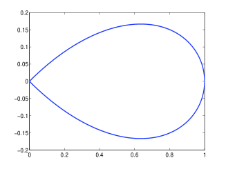
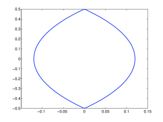
Figure 1: The curves $\mathcal{L}_{1}$, left, and $\mathcal{L}_{2}$, right. All corner points have the same opening angle $\omega=0.3\pi$.

Let $f_{1}$ and $f_{2}$ be the following functions

$$f_{1}(z)=-z|z|,$$

and

$$f_{2}(z)=\begin{cases}-1+iz&\text{ if }\textrm{Im}\,z<0\\ \quad\!1+iz&\text{ if }\textrm{Im}\,z\geq 0\end{cases}$$

The curves $\mathcal{L}_{1}$ and $\mathcal{L}_{2}$ have, respectively, one and two corner points of the magnitude $\omega\in(0,2\pi)$ each, and are defined by

$$\mathcal{L}_{j}:=\{t\in{\mathbb{C}}:t=\gamma_{j}(s),\quad s\in[0,1]\},\quad j=1,2.$$

where

$$\gamma_{1}(s) =\sin(\pi s)\exp(i\omega(s-0.5)),\quad s\in[0,1],$$

$$\gamma_{2}(s) =\begin{cases}\displaystyle-\frac{1}{2}\cot(\omega/2)+\frac{1}{2\sin(\omega/2)}\exp(i\omega(2s-0.5))&\text{ if}\;0\leq s\leq 1/2;\\[6.45831pt] \displaystyle\frac{1}{2}\cot(\omega/2)-\frac{1}{2\sin(\omega/2)}\exp(i\omega(2s-1.5))&\text{ if}\;1/2<s\leq 1.\end{cases}$$

The graphs of the curves $\mathcal{L}_{1}$ and $\mathcal{L}_{2}$ which are used in our examples below, are presented in Figure 1.

The right-hand side $f_{1}(z)$ is continuous on both curves $\mathcal{L}_{1}$ and $\mathcal{L}_{2}$, whereas $f_{2}(z)$ is discontinuous on both curves. Moreover, one of the discontinuity points of $f_{2}$ coincides with the angular point of $\mathcal{L}_{1}$.

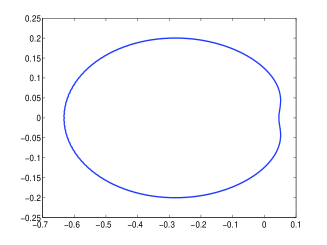
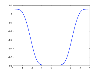
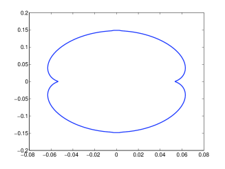
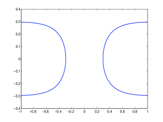
Figure 2: Approximate solutions of (3.3) with two different right hand sides and contours obtained by using method (3.5) with $n=512,d=16$. Left: Solutions in the case of continuous r.-h.s. $f_{1}(z)$. Right: Solutions in the case of discontinuous r.-h.s. $f_{2}(z)$. First row: Equations on $\mathcal{L}_{1}$. Second row: Equations on $\mathcal{L}_{2}$.

Approximate solutions of equation are obtained by the Nyström method (3.5) with $d=16$ and $\varepsilon_{p}=\delta_{p}$ and their graphs are presented in Figure 2. In the following table, the term $E_{n}^{(f_{k},\mathcal{L}_{j})}$ shows the relative error $\|x_{2n}-x_{n}\|_{2}/\|x_{2n}\|_{2}$ where $x_{n}$ is the approximate solution of the equation (3.3) for the contour $\mathcal{L}_{j}(0.3\pi),\;j=1,2$ with the right hand side $f_{k}$, $k=1,2$.

n	$E_{n}^{(f_{1},\mathcal{L}_{1})}$	$E_{n}^{(f_{1},\mathcal{L}_{2})}$	$E_{n}^{(f_{2},\mathcal{L}_{1})}$	$E_{n}^{(f_{2},\mathcal{L}_{2})}$
$32$	$2.5\times 10^{-3}$	$2.6\times 10^{-3}$	$1.5\times 10^{-2}$	$2.0\times 10^{-2}$
$96$	$8.3\times 10^{-4}$	$1.1\times 10^{-3}$	$7.5\times 10^{-3}$	$1.3\times 10^{-2}$
$256$	$3.1\times 10^{-4}$	$2.1\times 10^{-4}$	$4.0\times 10^{-3}$	$7.3\times 10^{-3}$

It is worth noting that a better convergence rate can be achieved by using certain modifications of the Nyström method [9, 10, 11] but the main focus of this paper is on the stability and on the angles the presence of which induces the instability of the Nyström method.

Let $(A_{n})$ be a bounded sequence of linear bounded operators $A_{n}:S_{n}^{d}\mapsto S_{n}^{d}$. The set $\mathcal{T}$ of such sequences equipped with componentwise operations of addition, multiplication, involution and multiplication by scalars, and with the norm

$$\|(A_{n})\|:=\sup\limits_{n\in{\mathbb{N}}}\|A_{n}\|$$

becomes a $C^{*}$-algebra.

Definition 3.1.

The sequence $(A_{n})\in\mathcal{T}$ is called stable if there is an $n_{0}\in{\mathbb{N}}$ such that for all $n\geq n_{0}$ the operators $A_{n}P_{n}:S_{n}^{d}(\Gamma)\mapsto S_{n}^{d}(\Gamma)$ are invertible and the norms $\|(A_{n}P_{n})^{-1}P_{n}\|_{n\geq n_{0}}$ are uniformly bounded.

Remark 3.2.

The stability of the method is directly connected to the condition numbers of the corresponding approximation methods. The graphs in Figure 3 show that the Nyström method for the double layer potential operator considered on the contours $\mathcal{L}_{1}(\omega)$, $\omega=0.25183\pi,\pi/3,\pi/4,\pi/2$ is stable. An abnormality of the graph in the case $\omega=0.25183\pi$ is caused by the proximity of this point to the so-called ”critical angle”. We refer the reader to Section 4 for a more detailed discussion of this phenomena.

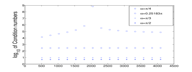
Figure 3: Condition numbers for some opening angles. The numbers of discretization points is $16n$.

It is well known (see, for example, [4, 16, 18]) that the stability of the approximation method $(A_{n})$ is equivalent to the invertibility of the coset $(A_{n})+\mathcal{G}$ in the quotient algebra $\mathcal{T}/\mathcal{G}$ where $\mathcal{G}$ is the set of all bounded sequences uniformly convergent to zero,

$$\mathcal{G}=\{(G_{n})\in\mathcal{T}:\lim\limits_{n\to\infty}\|G_{n}\|=0\}.$$

It turns out that in many cases the quotient algebra $\mathcal{T}/\mathcal{G}$ is too large to treat the invertibility problem efficiently. Therefore, one often considers a smaller algebra $\mathcal{A}\subset\mathcal{T}$ of sequences containing the approximation method in the question, at the same time expanding the ideal $\mathcal{G}$ to an ideal $\mathcal{J}$ in such a way that the initial problem will be equivalent to the invertibility of the corresponding coset in the quotient algebra $\mathcal{A}/\mathcal{J}$. More precisely, let $\mathcal{A}\subset\mathcal{T}$ denote the close subalgebra of $\mathcal{T}$ containing all sequences $(A_{n})$ such the strong limits

$$s-\lim\limits_{n\to\infty}A_{n}P_{n}=A\text{ and }s-\lim\limits_{n\to\infty}(A_{n})^{*}P_{n}=A^{*}$$

exist. Moreover, if $\mathcal{K}(L^{2}(\Gamma))$ is the set of all compact operators on $L^{2}(\Gamma)$, then the family of the sequences

$$\mathcal{J}=\{(J_{n}):J_{n}=P_{n}KP_{n}+G_{n},\;K\in\mathcal{K}(L^{2}(\Gamma)),\,G_{n}\in\mathcal{G}\}.$$

is a closed two-sided ideal of $\mathcal{A}$.

Theorem 3.3 (see [4, 16, 18]).

Assume that $(A_{n})\in\mathcal{A}$. Then the sequence $(A_{n})$ is stable if and only if the operator $A$ is invertible and the coset $(A_{n})+\mathcal{J}$ is invertible in the quotient algebra $\mathcal{A}/\mathcal{J}$.

This result can be used to study the applicability of the Nyström method to the double layer potential equations. Thus it follows from (3.2) that the sequence of approximation operators $(A_{n})_{n\in{\mathbb{N}}}$ corresponding to the Nyström method converges strongly to the operator $A_{\Gamma}$. Similar statement is valid for the sequence of adjoint operators. Let us show the invertibility of the coset $(A_{n})+\mathcal{J}$ in the quotient algebra $\mathcal{T}/\mathcal{J}$. It can be done by using local principles. Thus with each point $\tau\in\Gamma$ of the contour $\Gamma$ one can associate a simpler sequence of approximation operators $(A_{n}^{\tau})$, and the invertibility of the coset $(A_{n})+\mathcal{J}$ in $\mathcal{T}/\mathcal{J}$ is equivalent to the invertibility of cosets containing $(A_{n}^{\tau})$ in some algebra associated with the point $\tau$. For more detail we refer the reader to [4, 16]. Note that if $\tau\notin\mathcal{M}_{\Gamma}$ and $U_{\tau}\subset\Gamma$ is a neighbourhood of $\tau$ such that $\mathcal{M}_{\Gamma}\cap U_{\tau}=\emptyset$ and if $f_{\tau}$ is a function continuous on $\Gamma$ and such that

$$f_{\tau}(t)=\left\{\begin{array}[]{cl}1&\quad\text{if }t=\tau\\ 0&\quad\text{if }t\in\Gamma/U_{\tau},\\ \end{array}\right.$$

then the operator $f_{\tau}V_{\Gamma}f_{\tau}\in\mathcal{K}(L^{2}(\Gamma))$ [4, Corollary 4.6.3]). Therefore, the sequence $(A_{n}^{\tau})$ is locally equivalent to the sequence generated by the projections $(P_{n})$, so that the corresponding coset containing the sequence $(A_{n}^{\tau})$ is invertible. Thus one only has to identify and study the cosets associated with corner points of $\Gamma$. To this end, for each corner points $\tau_{j}\in\Gamma$ we consider the corresponding approximation method for the operator $A_{\omega_{j}}$ of (2.2) and approximate the integral $\int_{\Gamma_{j}}x(\tau)d\tau$ by a quadrature rule similar to (1.5), viz.,

$$\int_{\Gamma_{j}}x(\tau)d\tau\approx \sum\limits_{l=-\infty}^{-1}\sum\limits_{p=0}^{d-1}w_{p}x\left(\frac{l+\varepsilon_{p}}{n}e^{i(\beta_{j}+\omega_{j})}\right)\frac{e^{i(\beta_{j}+\omega_{j})}}{n}$$ (3.6)

$$+\sum\limits_{l=0}^{+\infty}\sum\limits_{p=0}^{d-1}w_{p}x\left(\frac{l+\varepsilon_{p}}{n}e^{i\beta_{j}}\right)\frac{e^{i\beta_{j}}}{n}$$

where $w_{p}$ and $\varepsilon_{p}$ as in (1.5). We also need spline spaces on the contours $\Gamma_{j}$ and ${\mathbb{R}}^{+}$. Let $S_{n}^{\beta_{j},\omega_{j}}$ be the smallest subspace of $L^{2}(\Gamma_{j})$ which contains all functions

$$\widetilde{\varphi}_{kn}(t)=\begin{cases}\begin{cases}\psi_{kn}(s)&\text{ if }t=se^{i\beta_{j}}\\ 0&\text{ otherwise }\end{cases},\quad k\leq 0,\vspace{0.5truecm}\\ \begin{cases}\psi_{k-d,n}(s)&\text{ if }t=se^{i(\beta_{j}+\omega_{j})}\\ 0&\text{ otherwise },\end{cases}\quad k<0,\end{cases}$$

where the basis splines $\psi_{kn}$ are defined by

$$\psi_{kn}(s):=\psi(ns-k),\quad s\in{\mathbb{R}},$$

and where the function $\psi:=u^{d}$ is obtained by recurrent relations

$$u^{l}(s) =\int_{\mathbb{R}}\chi_{[0,1)}(s-x)u^{l-1}(x)\,dx,\quad l=1,2,\ldots,d,$$

$$u^{0}(x) =\chi_{[0,1)}(x)=\left\{\begin{array}[]{cl}1&\quad\text{if}\quad x\in[0,1)\\ 0&\quad\text{otherwise}.\\ \end{array}\right.$$

The spline space $S_{n}({\mathbb{R}}^{+})=S_{n}^{d}({\mathbb{R}}^{+})$ is constructed similarly but we let $\beta_{j}=0$ and only take $\widetilde{\varphi}_{kn}$ for $k\geq 0$. Moreover, let $\widetilde{P}_{n}$ and $\widehat{P}_{n}$ denote the orthogonal projections from $L^{2}(\Gamma_{j})$ onto $S_{n}^{\beta_{j},\omega_{j}}$ and from $L^{2}({\mathbb{R}}^{+})$ onto $S_{n}({\mathbb{R}}^{+})$, respectively. Let ${\bf R}_{2}(\Gamma_{j})$ denote the set of functions on $\Gamma_{j}$ which are Riemann integrable on each finite part of $\Gamma_{j}$ and satisfy the condition

$$\|f\|_{{\bf R}} =\|f\|_{L^{2}(\Gamma_{j})}+\left(\sum\limits_{k=0}^{+\infty}\sup\limits_{t\in e^{i(\beta_{j}+\omega_{j})}[k,k+1]}|f(t)|^{2}\right)^{1/2}$$

$$+\left(\sum\limits_{k=0}^{+\infty}\sup\limits_{t\in e^{i\beta_{j}}[k,k+1]}|f(t)|^{2}\right)^{1/2}<+\infty.$$

Consider the integral equation

$$A_{\Gamma_{j}}x=f,\quad f\in{\bf R}_{2}(\Gamma_{j}).$$

As before, replace $x$ by an element $x_{n}\in S_{n}^{\beta_{j},\omega_{j}}$, apply quadrature formula (3.6) to the corresponding integrals and use the interpolation projections $\widetilde{Q}_{n}^{\delta}:{\bf R}(\Gamma_{j})\mapsto S_{n}^{\beta_{j},\omega_{j}}$ defined by

$$\widetilde{Q}_{n}^{\delta}x(t_{lp})=x(t_{lp}),\quad l\in{\mathbb{Z}},\;p=0,1,\ldots,d-1;$$

$$t_{lp}=\begin{cases}\displaystyle\frac{l+\delta_{p}}{n}e^{i(\beta_{j}+\omega_{j})}&\text{ if }l<0,\\[6.45831pt] \displaystyle\frac{l+\delta_{p}}{n}e^{i\beta_{j}}&\text{ if }l\geq 0.\end{cases}$$

As the result, we obtain the following operator equations

$$\widetilde{Q}_{n}^{\delta}A_{\Gamma_{j}}^{(\varepsilon,n)}\widetilde{P}_{n}x_{n}=\widetilde{Q}_{n}^{\delta}f,\quad x_{n}\in S_{n}^{\beta_{j},\omega_{j}},\;n\in{\mathbb{N}}.$$ (3.7)

These equations are equivalent to the infinite systems of linear algebraic equations

$$x_{n}(t_{kr}) +\frac{1}{2\pi i}\sum\limits_{l=-\infty}^{-1}\sum\limits_{p=0}^{d-1}w_{p}x_{n}(t_{lp})\left(\frac{\tau^{\prime}_{lp}}{\tau_{lp}-t_{kr}}-\frac{\overline{\tau^{\prime}_{lp}}}{\overline{\tau_{lp}}-\overline{t_{kr}}}\right)\frac{e^{i(\beta_{j}+\omega_{j})}}{n}$$

$$+\frac{1}{2\pi i}\sum\limits_{l=0}^{\infty}\sum\limits_{p=0}^{d-1}w_{p}x_{n}(t_{lp})\left(\frac{\tau^{\prime}_{lp}}{\tau_{lp}-t_{kr}}-\frac{\overline{\tau^{\prime}_{lp}}}{\overline{\tau_{lp}}-\overline{t_{kr}}}\right)\frac{e^{i\beta_{j}}}{n}$$

$$=f(t_{kr}),\quad k\in{\mathbb{Z}},\;p=0,1,\ldots,d-1$$

where $\tau_{lp}$ are defined analogously to $t_{lp}$ but the parameter $\delta_{p}$ is replaced by $\varepsilon_{p}$ and $\tau^{\prime}_{lp}=\gamma^{\prime}(l+\varepsilon_{p})/n.$

If one now uses the integral representation (2.1) of the Mellin convolution operator $\mathcal{M}(\mathbf{n}_{\omega_{j}})$ with the symbol $\mathbf{n}_{\omega_{j}}$ defined by (2.3), one can write the operator (3.7) in a different form. More precisely, let $\widehat{Q}_{n}^{\delta},n\in{\mathbb{N}}$ be the interpolation operators defined on the positive semi-axis.

Lemma 3.4.

If ${\bf k}_{\omega}$ is the function defined in (2.5), then the sequence $(\widetilde{Q}_{n}^{\delta}A_{\Gamma_{j}}^{(\varepsilon,n)}\widetilde{P}_{n})_{n\in{\mathbb{N}}}$ is stable if and only if the sequence $(\widehat{A}_{\omega_{j}}^{\varepsilon,\delta,n}\mathrm{diag}\,(\widehat{P}_{n},\widehat{P}_{n}))$,

$$\widehat{A}_{\omega_{j}}^{\varepsilon,\delta,n}\mathrm{diag}\,(\widehat{P}_{n},\widehat{P}_{n})=\begin{pmatrix}\widehat{P}_{n}&\widehat{Q}_{n}^{\delta}\mathcal{M}^{(\varepsilon,n)}({\bf k}_{\omega_{j}})\widehat{P}_{n}\\ \widehat{Q}_{n}^{1-\delta}\mathcal{M}^{(1-\varepsilon,n)}({\bf k}_{\omega_{j}})\widehat{P}_{n}&\widehat{P}_{n}\end{pmatrix}$$

is so.

Proof.

Let $\eta:L^{2}(\Gamma_{j})\mapsto L^{2}({\mathbb{R}}^{+})^{2}$ be the isomorphism defined in Section 2. It is easily seen that

$$\eta\widetilde{Q}_{n}^{\delta}\eta^{-1}=\mathrm{diag}\,(\widehat{Q}_{n}^{\delta},\widehat{Q}_{n}^{1-\delta}),\;\eta\widetilde{P}_{n}\eta^{-1}=\mathrm{diag}\,(\widehat{P}_{n},\widehat{P}_{n})$$

and

$$\eta A_{\Gamma_{j}}^{(\varepsilon,n)}\eta^{-1}=\eta\widetilde{P}_{n}\eta^{-1}+\eta V_{\Gamma_{j}}^{(\varepsilon,n)}\eta^{-1}=\begin{pmatrix}\widehat{P}_{n}&\mathcal{M}^{(\varepsilon,n)}({\bf k}_{\omega_{j}})\\ \mathcal{M}^{(1-\varepsilon,n)}({\bf k}_{\omega_{j}})&\widehat{P}_{n}\end{pmatrix}.$$

The obvious identity $\eta(\widetilde{Q}_{n}^{\delta}A_{\Gamma_{j}}^{(\varepsilon,n)}\widetilde{P}_{n})\eta^{-1}=(\eta\widetilde{Q}_{n}^{\delta}\eta^{-1})(\eta A_{\Gamma_{j}}^{(\varepsilon,n)}\eta^{-1})(\eta\widetilde{P}_{n}\eta^{-1})$ completes the proof. ∎

Let $l_{2}$ denote the space of sequences $(\xi_{j})_{j=0}^{\infty}$ of complex numbers $\xi_{j},j=0,1,\ldots$ such that $\big{(}\sum\limits_{j=0}^{\infty}|\xi_{j}|^{2}\big{)}^{1/2}<+\infty$. We now define the operators $E_{n}:l_{2}\mapsto S_{n}({\mathbb{R}}^{+})$ and $E_{-n}:S_{n}({\mathbb{R}}^{+})\mapsto l_{2}$ by

$$E_{n}((\xi_{j})_{j=0}^{\infty})=\sum\limits_{j=0}^{+\infty}\xi_{j}\widetilde{\varphi}_{jn}(t),\quad E_{-n}\left(\sum\limits_{j=0}^{+\infty}\xi_{j}\widetilde{\varphi}_{jn}(t)\right)=(\xi_{j})_{j=0}^{\infty}.$$

Recall [19] that the operators $E_{n}:l_{2}\mapsto S_{n}({\mathbb{R}}^{+})$ and $E_{-n}:S_{n}({\mathbb{R}}^{+})\mapsto l_{2}$ are bounded and there is a constant $C$ such that

$$||E_{n}||||E_{-n}||\leq C\,\text{ for all }\,n\in{\mathbb{N}}.$$

The last relation allows us to write the conditions of the stability of the sequence $(\widetilde{Q}_{n}^{\delta}A_{\Gamma_{j}}^{(\varepsilon,n)}\widetilde{P}_{n})_{n\in{\mathbb{N}}}$ in a more convenient form. By $\widehat{E}_{n}$ and $\widehat{E}_{-n}$ we, respectively, denote the diagonal operators,

$$\widehat{E}_{n}:=\mathrm{diag}\,(E_{n},E_{n}),\quad\widehat{E}_{-n}:=\mathrm{diag}\,(E_{-n},E_{-n}).$$

Corollary 3.5.

The sequence $(\widetilde{Q}_{n}^{\delta}A_{\Gamma_{j}}^{(\varepsilon,n)}\widetilde{P}_{n})_{n\in{\mathbb{N}}}$ is stable if and only if the operator $B_{\omega_{j},\delta,\varepsilon}=\widehat{E}_{-1}\widehat{A}_{\omega_{j}}^{\varepsilon,\delta,1}\mathrm{diag}\,(\widehat{P}_{1},\widehat{P}_{1})\widehat{E}_{1}$ is invertible.

Proof.

Straightforward calculations show that the entries of the approximation operator $\widehat{E}_{-n}\widehat{A}_{\omega_{j}}^{\varepsilon,\delta,n}\mathrm{diag}\,(\widehat{P}_{n},\widehat{P}_{n})\widehat{E}_{n}$ do not depend on $n$. Indeed, consider for example, the sequence $(E_{-n}\widehat{Q}_{n}^{\delta}\mathcal{M}^{(\varepsilon,n)}({\bf k}_{\omega_{j}})\widehat{P}_{n}E_{n})$. If $x_{n}\in\mathrm{im}\,\widehat{P}_{n}$, then

$$(\mathcal{M}^{(\varepsilon,n)}({\bf k}_{\omega_{j}})x_{n})(\sigma) =\sum\limits_{l=0}^{+\infty}\sum\limits_{p=0}^{d-1}w_{p}{\bf k}_{\omega_{j}}\left(\frac{\sigma}{\frac{l+\varepsilon_{p}}{n}}\right)\frac{1}{\frac{l+\varepsilon_{p}}{n}}\frac{1}{n}\,x_{n}\left(\frac{l+\varepsilon_{p}}{n}\right)$$

$$=\sum\limits_{p=0}^{d-1}w_{p}\sum\limits_{l=0}^{\infty}{\bf k}_{\omega_{j}}\left(\frac{\sigma}{\frac{l+\varepsilon_{p}}{n}}\right)\frac{1}{l+\varepsilon_{p}}\,x_{n}\left(\frac{l+\varepsilon_{p}}{n}\right),$$

and application of the interpolation operators $\widetilde{Q}_{n}^{\delta}$ leads to the relation

$$(\widetilde{Q}_{n}^{\delta}\mathcal{M}^{(\varepsilon,n)}({\bf k}_{\omega_{j}})x_{n})\left(\frac{k+\delta_{r}}{n}\right) =\sum\limits_{p=0}^{d-1}w_{p}\sum\limits_{l=0}^{\infty}{\bf k}_{\omega_{j}}\left(\frac{\frac{k+\delta_{r}}{n}}{\frac{l+\varepsilon_{p}}{n}}\right)\frac{1}{l+\varepsilon_{p}}\,x_{n}\left(\frac{l+\varepsilon_{p}}{n}\right)$$

$$=\sum\limits_{p=0}^{d-1}w_{p}\sum\limits_{l=0}^{\infty}{\bf k}_{\omega_{j}}\left(\frac{k+\delta_{r}}{l+\varepsilon_{p}}\right)\frac{1}{l+\varepsilon_{p}}\,x_{n}\left(\frac{l+\varepsilon_{p}}{n}\right).$$

Thus the entries of the operator $\widehat{E}_{-n}\widehat{A}_{\omega_{j}}^{\varepsilon,\delta,n}\mathrm{diag}\,(\widehat{P}_{n},\widehat{P}_{n})\widehat{E}_{n}$ do not depend on $n$. Therefore, the sequence in question is constant and one concludes that it is stable if and only if one of its members, say $E_{-1}\widehat{A}_{\omega_{j}}^{\varepsilon,\delta,1}\mathrm{diag}\,(\widehat{P}_{1},\widehat{P}_{1})E_{1}$, is invertible. This completes the proof. ∎

Theorem 3.6.

Let $n=qm,m\in{\mathbb{N}}$. Suppose that the operator $A$ is invertible. The Nyström method for the operator $A:L^{2}(\Gamma)\mapsto L^{2}(\Gamma)$ is stable if and only if all the operators $B_{\omega_{j},\delta,\varepsilon},j=0,1,\ldots,d-1$ are invertible.

Proof.

Let $\mathcal{C}$ denote the smallest closed $C^{*}$-algebra that contains the sequences $(P_{n}S_{\Gamma}P_{n})$, $(P_{n}MP_{n})$ and $(P_{n}fP_{n})$ where $f\in C(\Gamma)$ and let $\mathcal{J}$ be the ideal defined in Theorem 3.3. Then $(A^{(\varepsilon,n)}P_{n})\in\mathcal{C}$ and $\mathcal{C}/\mathcal{J}$ is a $C^{*}$-subalgebra of $\mathcal{A}/\mathcal{J}$. Therefore, the coset $(A^{(\varepsilon,n)}P_{n})+\mathcal{J}$ is invertible in $\mathcal{A}/\mathcal{J}$ if and only if it is invertible in $\mathcal{C}/\mathcal{J}$. However, the algebra $\mathcal{C}/\mathcal{J}$ has a nice centre and the invertibility of the coset $(A^{(\varepsilon,n)}P_{n})+\mathcal{J}$ in $\mathcal{C}/\mathcal{J}$ can be established by the Allan’s local principle [17] (see also [16, Theorem 1.9.5] for real algebra version of Allan’s local principle). Thus following the proof of Theorem 3.4 of [14] one can show that for any $\tau=\tau_{j}\in\mathcal{M}_{\Gamma}$ this coset is invertible if and only if the corresponding operator $B_{\omega_{j},\delta,\varepsilon}$ is invertible. On the other hand, it was already mentioned that for $\tau\notin\mathcal{M}_{\Gamma}$, the corresponding coset is always invertible, and application of Theorem 3.3 completes the proof. ∎

4 Numerical approach to the invertibility of local operators

Due to Theorem 3.6, the stability of the Nyström method depends on the invertibility of the operators $B_{\omega_{j},\delta,\varepsilon}$, $j=0,1,\ldots,q-1$. A more detailed study of these operators shows that they belong to an algebra of Toeplitz operators with matrix symbols. Unfortunately, at present there is no efficient criterion to check whether such operators are invertible or not. On the other hand, when considering the stability of approximation methods for Sherman–Lauricella and Muskhelishvili equations, a numerical approach to problems has been proposed in [12, 13]. Thus one can connect the invertibility of $B_{\omega,\delta,\varepsilon}$ with the stability of the method for the corresponding initial operator $A$ on model curves, which have one or more corner points all of the same magnitude $\omega$. As the next step, one can check the behaviour of the condition numbers for the method under consideration and decide which opening angles $\omega$ belong to the set of ”critical” angles, i.e to the set of the angles which cause the instability of the method. An essential difference to the situation with the Muskhelishvili and Sherman–Lauricella situation is that now one does not know whether the initial operator $A$ is invertible. Therefore the invertibility of $A$ has to be assumed from the very beginning or verified somehow. More precisely, one can apply Theorem 3.6 in a special setting and get the following result.

Theorem 4.1.

Let $\mathcal{L}=\mathcal{L}(\omega)$ denote any of two curves $\mathcal{L}_{1}(\omega)$ or $\mathcal{L}_{2}(\omega)$, $\omega\in(0,2\pi)$ defined in Section 3. If the corresponding operator $A_{\mathcal{L}(\omega)}$ of (3.3) is invertible, then the operator $B_{\omega,\delta,\varepsilon}$ is invertible if and only if the Nyström method $(Q_{n}^{\delta},A_{\mathcal{L}(\omega)}^{(\varepsilon,n)}P_{n})$ is stable.

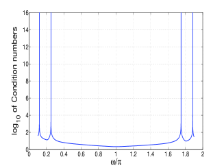
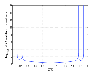
Figure 4: Condition numbers vs. opening angles in case $n=128,\,d=16$. Left: for one-corner curve, right: for two-corner curve

It is worth noting that the curves $\mathcal{L}_{1}$ and $\mathcal{L}_{2}$ have distinct shapes and the number of corner points. However, if their corner points have the same opening angle, the corresponding numerical experiments shall produce the same results. In what follows we are varying parameter $\omega$ in the interval $(0.1\pi,1.9\pi)$ and obtain two families of contours with one and two corner points, respectively. In order to find the instability angles, we divide the interval $[0.1\pi,1.9\pi]$ by the points $\omega_{k}=\pi*(0.1+0.001k)$. Further, for each point $\omega_{k}$ we compute the condition numbers for the Nyström method in the case where $n=128$ and the Gauss–Legendre quadrature with $d=16$ is used. Recall that both sets of parameters $\varepsilon_{p}$ and $\delta_{p}$ in (3.5) are the Gauss-Legendre points on the interval $[0,1]$. Calculating the corresponding condition numbers at the points $\omega_{k}$, we detected ”suspicious” points in the neighbourhoods of which condition numbers grow rapidly. Thereafter, in neighborhoods of such points the initial mesh has been refined and condition numbers are recalculated. The procedure is repeated until condition numbers reach the point $10^{16}$. The outcome of these computations is presented in Figure 4. Thus using both contours we found that the corresponding graphs have four peaks in the interval $(0.1,1.9)$, and approximate value for the critical ”angles are:

The case of one corner geometry, curve $\mathcal{L}_{1}$

$$0.11781222\pi,\quad 0.25164815\pi,\quad 1.74949877\pi,\quad 1.88430019\pi$$

The case of two corner geometry, curve $\mathcal{L}_{2}$

$$0.11780844\pi,\quad 0.25164706\pi,\quad 1.74840993\pi,\quad 1.88390254\pi.$$

Let us emphasize that for both the curve $\mathcal{L}_{1}$ and $\mathcal{L}_{2}$, the results obtained coincide up to three significant numbers. The peaks obtained are connected with four possible critical angles in the interval $(0.1\pi,1.9\pi)$. On the other hand, it is possible that they arose as the result of irreversibility of the corresponding operator $A$ on the curve $\mathcal{L}_{j}$. However, numerical experiments with other approximation methods for the same operators, which are not reported here, show that those methods have distinct critical angles. But it is not possible if the operator in question is irreversible for the angles mentioned. Thus the values found represent the ”critical” angles of the method but not the curves where the initial operator $A$ is not invertible.

Note that the numerical experiments are performed in MATLAB environment (version 7.9.0) and executed on an Acer Veriton M680 workstation equipped with a Intel Core i7 vPro 870 processor and 8GB of RAM.

5 Conclusion

In this work, necessary and sufficient conditions of the stability of the Nyström method for double layer potential equations on simple piecewise smooth contours are established. Moreover, we found four angles in the interval $(0.1\pi,1.9\pi)$ whose presence on the contour $\Gamma$ will cause the instability of the method, does not matter what the shape the curve $\Gamma$ has. Thus if the contour $\Gamma$ possesses at least one of such angles, the Nyström method is not stable and in order to find an approximate solution of the corresponding double layer potential equation, one has to use a different approximation method.

The results of numerical experiments are verified by using curves with different numbers of corner points and they are in a good correlation with theoretical studies.

References

[1]
K. E. Atkinson, The numerical
solution of integral equations of the second kind, Vol. 4 of Cambridge
Monographs on Applied and Computational Mathematics, Cambridge University
Press, Cambridge, 1997.
[2]
M. Costabel, Boundary integral
operators on Lipschitz domains: elementary results, SIAM J. Math. Anal.
19 (3) (1988) 613–626.
[3]
R. Kress, Linear integral
equations, 3rd Edition, Vol. 82 of Applied Mathematical Sciences, Springer,
New York, 2014.
[4]
S. Roch, P. A. Santos, B. Silbermann, Non-commutative Gelfand
theories, Universitext, Springer-Verlag London Ltd., London, 2011,
A tool-kit for operator theorists and numerical analysts.
[5]
G. Verchota, Layer
potentials and regularity for the Dirichlet problem for Laplace’s
equation in Lipschitz domains, J. Funct. Anal. 59 (3) (1984) 572–611.
[6]
G. A. Chandler, I. G. Graham, Uniform convergence of Galerkin
solutions to
noncompact integral operator equations, IMA J. Numer. Anal. 7 (3) (1987)
327–334.
[7]
V. D. Didenko, S. Roch, B. Silbermann,
Approximation methods for singular
integral equations with conjugation on curves with corners, SIAM J. Numer.
Anal. 32 (6) (1995) 1910–1939.
[8]
R. Kress, A Nyström method for boundary integral equations in
domains with
corners, Numer. Math. 58 (2) (1990) 145–161.
[9]
J. Bremer, On the
Nyström discretization of integral equations on planar curves with
corners, Appl. Comput. Harmon. Anal. 32 (1) (2012) 45–64.
[10]
J. Bremer, V. Rokhlin,
Efficient discretization
of Laplace boundary integral equations on polygonal domains, J. Comput.
Phys. 229 (7) (2010) 2507–2525.
[11]
J. Helsing, A. Holst, Variants of an explicit kernel-split
panel-based
nyström discretization scheme for helmholtz boundary value problems, Tech.
Rep. Arxiv:1311.6258v1, ArXiv (2013).
[12]
V. D. Didenko, J. Helsing, Stability
of the Nyström method for the Sherman-Lauricella equation, SIAM J.
Numer. Anal. 49 (3) (2011) 1127–1148.
[13]
V. D. Didenko, J. Helsing, Features of the Nyström method for
the
Sherman-Lauricella equation on piecewise smooth contours, East Asian J.
Appl. Math. 1 (4) (2011) 403–414.
[14]
V. D. Didenko, J. Helsing, On the
stability of the Nyström method for the Muskhelishvili equation on
contours with corners, SIAM J. Numer. Anal. 51 (3) (2013) 1757–1776.
[15]
N. I. Muskhelishvili, Singular integral equations, Nauka, Moscow,
1968.
[16]
V. D. Didenko, B. Silbermann, Approximation of additive
convolution-like
operators, Frontiers in Mathematics, Birkhäuser Verlag, Basel, 2008, Real
-algebra approach.
[17]
G. R. Allan, Ideals of vector-valued functions, Proc. London Math.
Soc.
18 (3) (1968) 193–216.
[18]
S. Prössdorf, B. Silbermann, Numerical analysis for integral and
related
operator equations, Birkhäuser Verlag, Berlin–Basel, 1991.
[19]
C. De Boor, A practical guide to splines, Springer Verlag,
New-York-Heidelberg-Berlin, 1978.