Symmetry breaking of solitons in two-dimensional complex potentials

Abstract

Symmetry breaking is reported for continuous families of solitons in the nonlinear Schrödinger equation with a two-dimensional complex potential. This symmetry-breaking bifurcation is forbidden in generic complex potentials. However, for a special class of partially parity-time-symmetric potentials, such symmetry breaking is allowed. At the bifurcation point, two branches of asymmetric solitons bifurcate out from the base branch of symmetry-unbroken solitons. Stability of these solitons near the bifurcation point are also studied, and two novel stability properties for the bifurcated asymmetric solitons are revealed. One is that at the bifurcation point, zero and simple imaginary linear-stability eigenvalues of asymmetric solitons can move directly into the complex plane and create oscillatory instability. The other is that the two bifurcated asymmetric solitons, even though having identical powers and being related to each other by spatial mirror reflection, can possess different types of unstable eigenvalues and thus exhibit non-reciprocal nonlinear evolutions under random-noise perturbations.

I Introduction

Parity-time ($\mathcal{PT}$) symmetric systems are dissipative systems with balanced gain and loss. The name of $\mathcal{PT}$symmetry was derived from non-Hermitian quantum mechanics with complex potentials [1]. This concept has since been applied to optics [2, 3], Bose-Einstein condensation [4], electric circuits [5], mechanical systems [6] and other settings. $\mathcal{PT}$-symmetric systems have some remarkable properties, such as all-real linear spectra [1, 7, 8, 9] and existence of continuous families of solitons [8, 10, 11, 12, 16, 13, 17, 18, 9, 19, 24, 14, 20, 21, 23, 25, 26, 15, 22, 27], which set them apart from other dissipative systems and make them resemble conservative systems. In multi-dimensions, the concept of $\mathcal{PT}$symmetry has been generalized to include partial parity-time ($\mathcal{PPT}$) symmetry, and it is shown that $\mathcal{PPT}$-symmetric systems share most of the properties of $\mathcal{PT}$systems [28]. Even some non-$\mathcal{PT}$-symmetric systems have been found to posesse certain properties of $\mathcal{PT}$systems, such as all-real linear spectra [29, 30, 31] and/or existence of soliton families [32, 33].

Symmetry-breaking bifurcation for continuous families of solitons in symmetric systems is a fascinating phenomenon. In conservative systems with real symmetric potentials, such symmetry breaking occurs frequently [34, 35, 36, 37, 38, 39, 40, 41, 42, 43]. That is, branches of asymmetric solitons can bifurcate out from the base branch of symmetric solitons when the power of symmetric solitons is above a certain threshold. But in $\mathcal{PT}$-symmetric complex potentials, such symmetry breaking is generically forbidden [44]. Mathematically the reason for this forbidden bifurcation is that this bifurcation requires infinitely many non-trivial conditions to be satisfied simultaneously, which is generically impossible. Intuitively this forbidden bifurcation can be understood as follows. Should it occur, continuous families of asymmetric solitons would be generated. Unlike in conservative systems, these asymmetric solitons in $\mathcal{PT}$systems would require not only dispersion-nonlinearity balancing but also gain-loss balancing, which is generically impossible. Surprisingly for a special class of one-dimensional (1D) $\mathcal{PT}$-symmetric potentials of the form $V(x)=g^{2}(x)+\alpha g(x)+ig^{\prime}(x)$, where $g(x)$ is a real even function and $\alpha$ a real constant, symmetry breaking of solitons was reported very recently [45]. This invites a natural question: can this symmetry breaking occur in 2D complex potentials? If so, what type of 2D complex potentials admit such symmetry breaking?

In this article, we study symmetry-breaking bifurcations of continuous families of solitons in 2D complex potentials. We show that in a special class of $\mathcal{PPT}$-symmetric separable potentials

$$V(x,y)=g^{2}(x)+\alpha g(x)+ig^{\prime}(x)+h(y),$$

where $g(x)$ is a real even function, $h(y)$ an arbitrary real function, and $\alpha$ a real constant, symmetry breaking can occur. Specifically, from a base branch of $\mathcal{PPT}$-symmetric solitons and above a certain power threshold, two branches of asymmetric solitons with identical powers can bifurcate out. At the bifurcation point, the base branch of $\mathcal{PPT}$-symmetric solitons changes stability, analogous to conservative systems. However, the bifurcated asymmetric solitons can exhibit new stability properties which have no counterparts in conservative systems. One novel property is that at the bifurcation point, the zero and simple imaginary eigenvalues in the linear-stability spectra of asymmetric solitons can move directly into the complex plane and create oscillatory instability. Another novel property is that the two asymmetric solitons can possess different types of linear-instability eigenvalues. As a consequence, these two asymmetric solitons, which are related to each other by spatial mirror reflection, can exhibit non-reciprocal evolutions under random-noise perturbations.

II Symmetry breaking of solitons

Nonlinear beam propagation in an optical medium with gain and loss can be modeled by a nonlinear Schrödinger equation [46]

$$i\Psi_{z}+\nabla^{2}\Psi+V(x,y)\Psi+\sigma|\Psi|^{2}\Psi=0,$$ (2.1)

where $z$ is the propagation distance, $(x,y)$ is the transverse plane, $\nabla^{2}=\partial_{xx}+\partial_{yy}$, $V(x,y)$ is a complex potential, and $\sigma=\pm 1$ is the sign of nonlinearity.

Solitons in Eq. (2.1) are sought of the form

$$\Psi(x,y,z)=e^{i\mu z}\psi(x,y),$$ (2.2)

where $\mu$ is a real propagation constant, and $\psi(x,y)$ is a localized function solving the equation

$$\nabla^{2}\psi+V(x,y)\psi+\sigma|\psi|^{2}\psi=\mu\psi.$$ (2.3)

If the complex potential $V(x,y)$ is $\mathcal{PT}$-symmetric or $\mathcal{PPT}$-symmetric, continuous families of $\mathcal{PT}$-symmetric or $\mathcal{PPT}$-symmetric solitons are admitted [18, 28], but symmetry breaking of such solitons is generically forbidden [44]. However, for certain special forms of 1D $\mathcal{PT}$potentials, symmetry breaking of 1D solitons has been reported very recently [45].

In this article, we show that symmetry breaking of 2D solitons is also possible in the model (2.1) for a special class of complex potentials

$$V(x,y)=g^{2}(x)+\alpha g(x)+ig^{\prime}(x)+h(y),$$ (2.4)

where $g(x)$ is a real even function, i.e.,

$$g(-x)=g(x),$$

$h(y)$ is an arbitrary real function, and $\alpha$ is a real constant. This potential is separable in $(x,y)$, and its imaginary part is $y$-independent. In addition, this potential is $\mathcal{PPT}$-symmetric, i.e.,

$$V^{*}(x,y)=V(-x,y),$$ (2.5)

where the asterisk represents complex conjugation. Due to separability of this potential, it is easy to see that its linear spectrum can be all-real [28]. Note that a potential of the form (2.4) but with $x$ and $y$ switched is equivalent to (2.4) and thus does not deserve separate consideration.

The $x$-component of the separable potential (2.4) is the same as the 1D complex potential for symmetry breaking as reported in [45], but the $y$-component of this separable potential is real and quite different. Should this $y$-component be complex and also take the form of its $x$-component, we have found that symmetry breaking would no longer occur. This indicates that symmetry breaking in the special 2D potential (2.4) is by no means obvious and cannot be anticipated from the 1D potential for symmetry breaking in [45].

Below we use two explicit examples of the potential (2.4) to demonstrate symmetry breaking of 2D solitons and reveal their unique linear-stability properties.

Example 1   In our first example, we take the potential (2.4) with

$$g(x)=0.3\left[e^{-(x+1.2)^{2}}+e^{-(x-1.2)^{2}}\right],$$ (2.6)

$$\alpha=10,\quad h(y)=0.$$ (2.7)

This is a $y$-independent stripe potential which is illustrated in Fig. 1. The spectrum of this potential is all-real, and all eigenvalues lie in the continuous spectrum of $(-\infty,\hskip 0.56917pt2.0569]$.

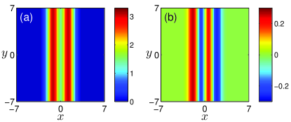
Figure 1: A stripe complex potential (2.4) with (2.6)-(2.7) in Example 1. (a) Re($V$); (b) Im($V$).

Solitons in Eq. (2.3) under this potential will be computed by the Newton-conjugate-gradient method. This method features high accuracy as well as fast speed. The application of this method for solitons in conservative systems has been described in [47, 48]. In those cases, the linear Newton-correction equation was self-adjoint and thus could be solved directly by preconditioned conjugate gradient iterations. However, the present equation (2.3) is dissipative, hence the resulting Newton-correction equation is non-self-adjoint. In this case, direct conjugate gradient iterations on this equation would fail, and it is necessary to turn this equation into a normal equation and then solve it by preconditioned conjugate gradient iterations. In the appendix, this Newton-conjugate-gradient method for Eq. (2.3) is explained in more detail. In addition, a simple Matlab code is displayed.

Using this Newton-conjugate-gradient method, we find that from the edge of the continuous spectrum $\mu_{0}=2.0569$, a continuous family of solitons $\psi_{s}(x,y;\mu)$, localized in both $x$ and $y$ directions, bifurcate out. The power curve of this soliton family is displayed in Fig. 2 (blue curve in the first row). Here the power is defined as

$$P(\mu)=\int_{-\infty}^{\infty}\int_{-\infty}^{\infty}|\psi(x,y;\mu)|^{2}dxdy.$$

At two points ‘a,b’ of this power curve, soliton profiles are shown in Fig. 2 (the second and third rows). These solitons respect the same $\mathcal{PPT}$symmetry of the potential, i.e.,

$$\psi_{s}^{*}(x,y)=\psi_{s}(-x,y).$$ (2.8)

The existence of this soliton family respecting the same symmetry of the potential is anticipated.

What is surprising is that, when the power of this soliton family reaches a critical value $P_{c}\approx 8.60$, two branches of asymmetric solitons bifurcate out through a pitchfork bifurcation. These asymmetric solitons do not respect the $\mathcal{PPT}$symmetry (2.8). At the same $\mu$ value, they have identical powers and are related to each other through a spatial reflection

$$\psi_{a}^{(1)*}(x,y)=\psi_{a}^{(2)}(-x,y).$$ (2.9)

The power curve of these two branches of asymmetric solitons is plotted in Fig. 2 (red curve in the first row). Notice that unlike the symmetric (base) branch, the power slope of these asymmetric branches is negative at the bifurcation point. At point ‘c’ of the asymmetric branches, the profile for one of the two asymmetric solitons is displayed in Fig. 2 (the bottom row). Asymmetry in its profile can clearly be seen. These solitons have lost the $\mathcal{PPT}$symmetry of the underlying potential, thus symmetry breaking has occurred.

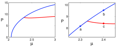
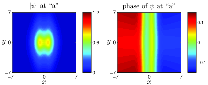
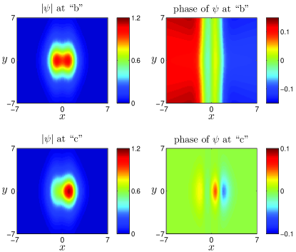
Figure 2: Symmetry breaking of solitons in Example 1. First row: power curves of symmetric (blue) and asymmetric (red) solitons; the right panel is an amplification of the left panel around the bifurcation point. Second to fourth rows: soliton profiles at points ‘a,b,c’ of the power curve; left panels: amplitude fields; right panels: phase fields.

Next we analyze linear stability of these symmetric and asymmetric solitons. To determine linear stability, we perturb these solitons as

$$\Psi(x,y,z)=e^{i\mu z}\left[\psi(x,y)+\tilde{u}(x,y)\hskip 1.42271pte^{\lambda z}+\tilde{w}^{*}(x,y)\hskip 1.42271pte^{\lambda^{*}z}\right],$$

where $|\tilde{u}|,|\tilde{w}|\ll|\psi|$. After substitution into equation (2.1) and linearizing, we arrive at the eigenvalue problem

$${\cal L}\left(\begin{array}[]{c}\tilde{u}\\ \tilde{w}\end{array}\right)=\lambda\left(\begin{array}[]{c}\tilde{u}\\ \tilde{w}\end{array}\right),$$ (2.10)

where

$${\cal L}=i\left(\begin{array}[]{c c}{\cal L}_{11}&{\cal L}_{12}\\ {\cal L}_{21}&{\cal L}_{22}\end{array}\right),$$

and

$${\cal L}_{11} =\nabla^{2}+V-\mu+2\sigma|\psi|^{2},$$

$${\cal L}_{12} =\sigma\psi^{2},$$

$${\cal L}_{21} =-\sigma\left(\psi^{2}\right)^{*},$$

$${\cal L}_{22} =-\left(\nabla^{2}+V-\mu+2\sigma|\psi|^{2}\right)^{*}.$$

If eigenvalues with positive real parts exist, the soliton is linearly unstable; otherwise it is linearly stable.

Linear-stability eigenvalues exhibit important differences for symmetric and asymmetric solitons. For symmetric solitons $\psi_{s}(x,y)$, it is easy to show from soliton symmetry (2.8) and potential symmetry (2.5) that if

$$\lambda,\,\tilde{u}(x,y),\,\tilde{w}(x,y)$$

is an eigenmode, then so is

$$\lambda^{*},\,\tilde{w}^{*}(x,y),\,\tilde{u}^{*}(x,y),$$

$$-\lambda,\,\tilde{w}(-x,y),\,\tilde{u}(-x,y),$$

and

$$-\lambda^{*},\,\tilde{u}^{*}(-x,y),\,\tilde{w}^{*}(-x,y).$$

Thus for symmetric solitons, real and imaginary eigenvalues appear as pairs $(\lambda,-\lambda)$, and complex eigenvalues appear as quartets $\{\lambda,\lambda^{*},-\lambda,-\lambda^{*}\}$.

For asymmetric solitons, however, the situation is different. While it is still true that if $\lambda$ is an eigenvalue, so is $\lambda^{*}$, but due to the lack of soliton symmetry (2.8), $-\lambda$ and $-\lambda^{*}$ are no longer eigenvalues. In other words, for asymmetric solitons, complex eigenvalues appear as conjugate pairs $(\lambda,\lambda^{*})$, not as quartets; and real eigenvalues appear as single eigenvalues, not as $(\lambda,-\lambda)$ pairs. These differences on eigenvalue symmetry between symmetric and asymmetric solitons will have important implications, as we will see later in this section.

For the two branches of asymmetric solitons, their linear-stability eigenvalues are related. Indeed, from the mirror symmetry (2.9) between these two bifurcated soliton branches, it is easy to see that if $\lambda$ is an eigenvalue of the soliton $\psi_{a}^{(1)}(x,y;\mu)$, then $-\lambda^{*}$ will be an eigenvalue of the companion soliton $\psi_{a}^{(2)}(x,y;\mu)$. In other words, linear-stability spectrum of the soliton $\psi_{a}^{(1)}(x,y;\mu)$ is a mirror reflection of that spectrum of the companion soliton $\psi_{a}^{(2)}(x,y;\mu)$ around the imaginary axis.

The eigenvalue problem (2.10) can be computed by the Fourier collocation method (for the full spectrum) or the Newton-conjugate-gradient method (for individual discrete eigenvalues) [48]. We find that near the symmetry-breaking bifurcation point $\mu_{c}\approx 2.33$, symmetric solitons are stable before the bifurcation point ($\mu<\mu_{c}$) and unstable after it ($\mu>\mu_{c}$), and both branches of asymmetric solitons are unstable. This stability behavior is marked on the power curve in Fig. 3 (upper left panel). To shed light on the origins of these stabilities and instabilities, linear-stability spectra at three points ‘a,b,c’ of this power curve, for the three solitons displayed in Fig. 2, are displayed in panels (a,b,c) of Fig. 3 respectively. We see from panel (a) that before the bifurcation, the symmetric soliton has a pair of discrete eigenvalues on the imaginary axis. At the bifurcation point, this pair of imaginary eigenvalues coalesce at the origin. After bifurcation, these coalesced eigenvalues split along the real axis in opposite directions for both symmetric and asymmetric solitons. Along the symmetric branch, the two split eigenvalues form a $(\lambda,-\lambda)$ pair [see panel (b)]. But along the asymmetric branches, the two split eigenvalues do not form a $(\lambda,-\lambda)$ pair since they have different magnitudes [see panel (c)]. These spectra show that the instability of symmetric and asymmetric solitons after bifurcation is due to the zero-eigenvalue splitting along the real axis at $\mu=\mu_{c}$, and this instability is exponential (caused by real eigenvalues).

It is interesting to observe that the power-curve structure and the associated stability behaviors in Fig. 3 (upper left panel) resemble that in the conservative generalized nonlinear Schrödinger equations with real potentials (see Fig. 2c in Ref. [43]). In that conservative case, it was shown that if the power slopes of the symmetric and asymmetric solitons at the bifurcation point have opposite signs, then both solitons will share the same stability or instability [43]. Fig. 3 of the present article suggests that such a statement might hold for complex potentials as well. But whether it holds for other complex potentials merits further investigation.

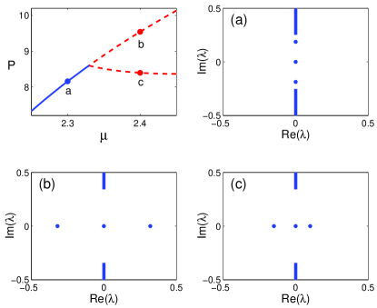
Figure 3: Linear-stability behaviors of solitons near the symmetry-breaking point in Example 1. Upper left panel: the power curve with stability marked (solid blue for stable and dashed red for unstable). Panels (a,b,c): linear-stability spectra for the solitons at points ‘a,b,c’ of the power curve.

The linear-stability results of Fig. 3 are corroborated by nonlinear evolution simulations of those solitons under random-noise perturbations. To demonstrate, we perturb the three solitons of Fig. 2 by 1% random-noise perturbations, and their nonlinear evolutions are displayed in Fig. 4. As can be seen, the perturbed symmetric soliton before bifurcation shows little change even after $z=100$ units of propagation, confirming that it is linearly stable (see top row of Fig. 4). The perturbed symmetric soliton after bifurcation, on the other hand, clearly breaks up and evolves into a highly asymmetric profile after 20 units of propagation, confirming that it is linearly unstable (see middle row of Fig. 4). The perturbed asymmetric soliton, whose initial intensity hump is located at the right side, also breaks up and evolves into a profile whose intensity hump moves to the left side after 50 units of propagation, confirming that it is linearly unstable as well (see bottom row of Fig. 4).

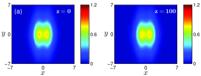
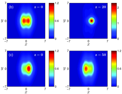
Figure 4: Nonlinear evolutions of the three solitons in Fig. 2 under 1% random-noise perturbations (locations of these solitons on the power curve are marked in both Figs. 2 and 3).

Example 2   In our second example, we take the potential (2.4) with

$$g(x)=0.3\left[e^{-(x+1.2)^{2}}+e^{-(x-1.2)^{2}}\right],\quad\alpha=10,$$

and

$$h(y)=2\left[e^{-(y+1.2)^{2}}+0.8\hskip 0.56917pte^{-(y-1.2)^{2}}\right].$$

This potential is illustrated in Fig. 5. Its real part is no longer a stripe potential, neither is it symmetric in $y$. The spectrum of this potential is all-real, and it consists of three discrete eigenvalues of $\{2.5643,2.5689,3.2028\}$ and the continuous spectrum of $(-\infty,2.0569]$.

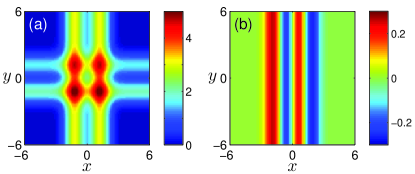
Figure 5: The $\mathcal{PPT}$-symmetric complex potential (2.4) in Example 2. (a) Re($V$); (b) Im($V$).

From the largest discrete eigenvalue of $\mu_{0}=3.2028$, a continuous family of $\mathcal{PPT}$-symmetric solitons bifurcates out. The power curve of this soliton family is plotted in Fig. 6(A) (blue curve). When the power of these solitons reaches a threshold of $P_{c}\approx 5.24$ (at $\mu_{c}\approx 3.56$), two branches of asymmetric solitons bifurcate out, whose power curves are also displayed in Fig. 6(A) (red curve). As before, these two asymmetric solitons are related to each other by

$$\psi_{a}^{(1)*}(x,y)=\psi_{a}^{(2)}(-x,y),$$ (2.11)

thus they have identical powers. Enlargement of this power curve near the bifurcation point is shown in Fig. 6(B). At points ‘a,b,c,d’ of this amplified power diagram, the solitons’ amplitude profiles are plotted in Fig. 6 (middle and bottom rows). Here points ‘c,d’ are the same power points but on different asymmetric-soliton branches. We can see that solitons at points ‘a,b’ of the base branch are $\mathcal{PPT}$-symmetric, with ‘a’ before bifurcation and ‘b’ after it. The solitons at point ‘c,d’ of the bifurcated branches, however, are asymmetric, with the energy concentrated on the right and left side of the $x$-axis respectively. In this example, power slopes of the base and bifurcated soliton branches have the same sign at the bifurcation point, which is different from Example 1.

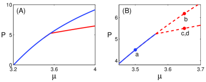
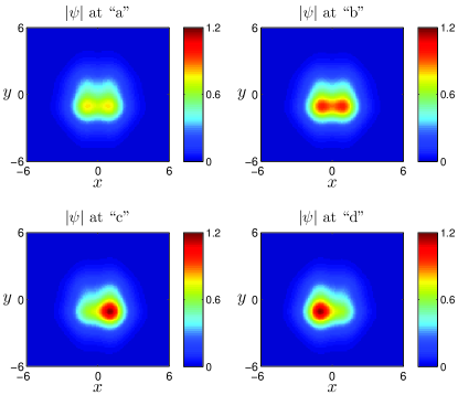
Figure 6: Symmetry breaking of solitons in Example 2. (A) power curves of $\mathcal{PPT}$-symmetric (blue) and asymmetric (red) solitons; (B) enlargement of the left power curves near the bifurcation point (solid blue indicates linearly-stable branch, and dashed red indicates linearly-unstable branches). Middle and bottom rows: profiles of soliton amplitudes at points ‘a,b,c,d’ of the power curve.

Now we discuss linear-stability behaviors of solitons in Example 2. For the base branch of $\mathcal{PPT}$-symmetric solitons, they are linearly stable before the bifurcation point and linearly unstable after it, which is similar to Example 1 and is not surprising. To illustrate, linear-stability spectra for the two $\mathcal{PPT}$-symmetric solitons at points ‘a,b’ of the power curve in Fig. 6(B) are plotted in Fig. 7(a,b) respectively. At point ‘a’ (before bifurcation), all eigenvalues are imaginary, indicating linear stability. At point ‘b’ (past bifurcation), a pair of real eigenvalues $\pm 0.3704$ appear, which makes this $\mathcal{PPT}$-symmetric soliton linearly unstable. What happens is that when the power of the base branch crosses the bifurcation point, a pair of imaginary eigenvalues collide at the origin and then bifurcate out of the origin along the real axis, creating a $\pm\lambda$ pair of real eigenvalues and hence instability.

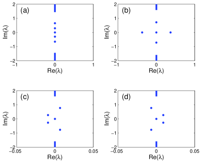
Figure 7: (a-d): Linear-stability spectra for solitons at points ‘a-d’ of the power curve in Fig. 6(B).

The most interesting new phenomena in Example 2 are linear-stability behaviors of asymmetric solitons. We find that both branches of asymmetric solitons are linearly unstable, but origins of their instabilities are different. To demonstrate, linear-stability spectra for the two asymmetric solitons at points ‘c,d’ of Fig. 6(B) are plotted in Fig. 7(c,d). These two spectra are related to each other by mirror reflection around the imaginary axis, as we have pointed out earlier in the text. In addition, eigenvalues of these asymmetric solitons must appear in conjugate pairs $(\lambda,\lambda^{*})$, but no other eigenvalue symmetry exists.

The first phenomenon we notice in these spectra is that, both asymmetric solitons are linearly unstable due to oscillatory instabilities caused by complex eigenvalues. The second phenomenon is that, even though these spectra contain complex eigenvalues, these eigenvalues do not appear in quartets $\{\lambda,\lambda^{*},-\lambda,-\lambda^{*}\}$. This contrasts asymmetric solitons in real (conservative) potentials, where complex eigenvalues must appear in quartets.

The third and probably most noteworthy phenomenon in these spectra is that, unstable eigenvalues in these two asymmetric solitons have different origins. Indeed, before the bifurcation, $\mathcal{PPT}$-symmetric solitons on the base branch have two pairs of simple discrete imaginary eigenvalues [see Fig. 7(a)]. At the bifurcation point, the smaller pair of simple imaginary eigenvalues coalesce at the origin, while the larger pair remain on the imaginary axis. When asymmetric solitons bifurcate out from the base branch, for the one with energy concentrated on the right side (see Fig. 6, at point ‘c’), the pair of simple eigenvalues on the imaginary axis move directly to the right half plane, creating oscillatory instability [see Fig. 7(c)]. The coalesced zero eigenvalues at the origin, on the other hand, move leftward into the complex plane, creating a conjugate pair of stable complex eigenvalues [see Fig. 7(c)]. For the asymmetric soliton with energy concentrated on the left side, the situation is just the opposite [see Fig. 7(d)]. Thus the origin of instability for one branch of asymmetric solitons is due to a pair of simple imaginary eigenvalues moving directly off the imaginary axis, while the origin for the other branch of asymmetric solitons is due to the zero eigenvalue moving to the complex plane.

The above phenomenon of zero and simple imaginary eigenvalues moving directly into the complex plane and creating oscillatory instability in solitons is very novel, since it contrasts conservative systems with real potentials. In real potentials, linear-stability complex eigenvalues of solitons appear as quartets $\{\lambda,\lambda^{*},-\lambda,-\lambda^{*}\}$. Partly because of it, bifurcation of complex eigenvalues off the imaginary axis typically occurs through collision of imaginary eigenvalues of opposite Krein signatures (a bifurcation referred to as Hamiltonian-Hopf bifurcation in the literature [49]). In addition, complex eigenvalues (not on the real and imaginary axes) cannot bifurcate from the origin when two simple eigenvalues collide there. But in complex potentials, the situation can be very different as is explained above.

The fourth phenomenon in the spectra of Fig. 7 is that, the maximal growth rates of perturbations in these two asymmetric solitons are different. Indeed the unstable eigenvalues in Fig. 7(c) are $0.0067\pm 0.7721i$, giving a growth rate of $0.0067$; while the unstable eigenvalues in Fig. 7(d) are $0.0090\pm 0.2692i$, giving a larger growth rate of 0.0090. The fifth phenomenon is that these oscillatory instabilities in asymmetric solitons are rather weak due to these small growth rates. This means that these oscillatory instabilities will take long distances to develop.

Of the five phenomena mentioned above, the third and fourth ones are the most fundamental, and they are rarely seen (if ever) for asymmetric solitons arising from symmetry-breaking bifurcations.

Since the two branches of asymmetric solitons have different origins of instability and different growth rates, small perturbations in these solitons will grow differently, leading to non-reciprocal developments of instability. To demonstrate, evolutions of the two asymmetric solitons in Fig. 6 under 1% random-noise perturbations are displayed in Fig. 8. We see that even though these two asymmetric solitons are related to each other by a mirror reflection (2.11) and are reciprocal, their evolutions under weak perturbations are not reciprocal. Indeed, after 1000 distance units of propagation, they reach similar asymmetric states. This non-reciprocal evolution is most visible in Fig. 8(c,d), where amplitude evolutions at spatial positions $(x,y)=(-1.2,-1.2)$ and $(1.2,-1.2)$ for the two perturbed asymmetric solitons are plotted respectively. These amplitude evolutions vividly confirm that (a) the two asymmetric solitons are linearly unstable; (b) their instabilities are caused by different unstable modes with different growth rates; and (c) the nonlinear evolutions are non-reciprocal even though the asymmetric solitons are.

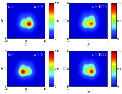
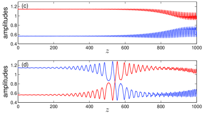
Figure 8: Non-reciprocal evolutions of two reciprocal asymmetric solitons in Fig. 6 under 1% random-noise perturbations in Example 2. First and second rows: initially perturbed asymmetric solitons and their evolved solutions at $z=1000$. (c,d) Evolutions of solution amplitudes $|\Psi|$ versus $z$ at two spatial positions $(x,y)=(-1.2,-1.2)$ (blue) and $(1.2,-1.2)$ (red) for the two asymmetric solitons of Fig. 6 under perturbations.

In Example 2, when asymmetric solitons bifurcate out, the coalesced zero eigenvalue and the pair of imaginary eigenvalues move in opposite directions in the complex plane, causing instability to both asymmetric solitons [see Fig. 7(c,d)]. For other potentials and/or nonlinearities, if those eigenvalues bifurcate in the same direction, then one asymmetric soliton would be linearly stable and the other unstable. Such a scenario would be very remarkable. Whether such scenarios exist or not is an open question.

In the above two examples, symmetry breaking was observed for complex potentials of the form (2.4). We have also tried a related class of complex potentials

$$V(x,y)=g^{2}(x)+\alpha g(x)+ig^{\prime}(x)+h^{2}(y)+\beta\hskip 0.85355pth(y)+ih^{\prime}(y),$$ (2.12)

where $g(x),h(y)$ are real even functions, and $\alpha,\beta$ are real constants. This potential is $\mathcal{PT}$-symmetric, i.e., $V^{*}(x,y)=V(-x,-y)$, and it admits $\mathcal{PT}$-symmetric solitons. But we did not find symmetry breaking here, i.e., we did not find branches of asymmetric solitons bifurcating from the branch of $\mathcal{PT}$-symmetric solitons.

Why does symmetry breaking occur in potentials of the form (2.4) but not in some others such as (2.12)? This question is not clear yet. In fact, even for one-dimensional symmetry-breaking bifurcations reported in [45], the reason for that symmetry breaking was not entirely clear either. In the 1D case, the forms of potentials for symmetry breaking in $\mathcal{PT}$-symmetric potentials and for soliton families in asymmetric potentials are the same [45, 32]. For those potentials, there is a conserved quantity which, when combined with a shooting argument, helps explain the existence of soliton families in asymmetric complex potentials [33]. That conserved quantity may prove useful to explain symmetry breaking in those 1D potentials as well.

For the present class of 2D potentials (2.4), we have found that Eq. (2.1) also admits a conservation law

$$Q_{t}+J_{x}+K_{y}=0,$$ (2.13)

where

$$Q=i\Psi(\Psi_{x}^{*}-i\hat{g}\Psi^{*}),$$

$$J=\Psi\Psi_{yy}^{*}+|\Psi_{x}+i\hat{g}\Psi|^{2}-i\Psi\Psi_{t}^{*}+\left(h-\frac{\alpha^{2}}{4}\right)|\Psi|^{2}+\frac{\sigma}{2}|\Psi|^{4},$$

$$K=\Psi_{y}(\Psi_{x}^{*}-i\hat{g}\Psi^{*})-\Psi(\Psi_{x}^{*}-i\hat{g}\Psi^{*})_{y},$$

and

$$\hat{g}(x)=g(x)+\frac{\alpha}{2}.$$

For solitons (2.2), substituting their functional form into the above conservation law, a reduced conservation law for the soliton function $\psi(x,y)$ can also be derived. For the other class of potentials (2.12), however, we could not find such a conservation law. This suggests that there is indeed a connection between the existence of a conservation law and the presence of symmetry breaking of solitons. But this connection in the 2D case would be harder to establish since shooting-type arguments would break down.

In 1D, symmetry breaking in symmetric potentials and existence of soliton families in asymmetric potentials occur in complex potentials of the same form [45, 32]. This invites a natural question: for the class of 2D complex potentials (2.4) which admits symmetry breaking, if these potentials are not $\mathcal{PPT}$-symmetric, i.e., if $g(x)$ is real but not even, can they support continuous families of solitons? The answer is positive as our preliminary numerics has shown.

III Summary and Discussion

In this article, we reported symmetry breaking of solitons in the nonlinear Schrödinger equation with a class of two-dimensional $\mathcal{PPT}$-symmetric complex potentials (2.4). At the bifurcation point, two branches of asymmetric solitons bifurcate out from the base branch of $\mathcal{PPT}$-symmetric solitons, and this bifurcation is quite surprising. Stability of these solitons near the bifurcation point were also studied. In the two examples we investigated, we found that the base branch of symmetric solitons changes stability at the bifurcation point, and the bifurcated asymmetric solitons are unstable. For the asymmetric solitons, two novel stability properties were further revealed. One is that at the bifurcation point, the zero and simple imaginary linear-stability eigenvalues of asymmetric solitons can move directly into the complex plane and create oscillatory instability. The other is that the two bifurcated asymmetric solitons, even though having identical powers and being related to each other by spatial mirror reflection, can have different origins of linear instability and thus exhibit non-reciprocal nonlinear evolutions under random-noise perturbations.

We should point out that the complex potentials (2.4) possess a single ($\mathcal{PPT}$) symmetry, thus they must be in that special form in order for symmetry breaking to occur. If a complex potential exhibits more than one spatial symmetry, say double $\mathcal{PPT}$symmetries

$$V^{*}(x,y)=V(-x,y),\quad V^{*}(x,y)=V(x,-y),$$

or one $\mathcal{PT}$and one $\mathcal{PPT}$symmetry, say

$$V^{*}(x,y)=V(-x,-y),\quad V^{*}(x,y)=V(-x,y),$$

then this potential can admit symmetry breaking without the need for special functional forms (this prospect has been mentioned in [44] and confirmed by our own numerics). When symmetry breaking occurs in such double-symmetry potentials, the base branch of solitons respect both symmetries of the potential, while the bifurcated solitons lose one symmetry but retain the other. The simple mathematical reason for symmetry breakings in double-symmetry potentials is that the infinitely many analytical conditions for symmetry breaking in [44] are all satisfied automatically due to the remaining symmetry of the bifurcated solitons. That situation is fundamentally different from symmetry breakings in potentials of special forms such as (2.4), which admit a single spatial symmetry. The mathematical reason for symmetry breaking in single-symmetry potentials of special functional forms such as (2.4) is still not clear.

Appendix: A Numerical Method for Computing Solitons in Complex Potentials

In this appendix, we describe the Newton-conjugate-gradient method for computing solitons in Eq. (2.3) with a complex potential.

The general idea of the Newton-conjugate-gradient method is that, for a nonlinear real-valued vector equation

$$\textbf{L}_{0}(\textbf{u})=0,$$ (A.1)

its solution u is obtained by Newton iterations

$$\textbf{u}_{n+1}=\textbf{u}_{n}+\Delta\textbf{u}_{n},$$ (A.2)

where the updated amount $\Delta\textbf{u}_{n}$ is computed from the linear Newton-correction equation

$$\textbf{L}_{1n}\Delta\textbf{u}_{n}=-\textbf{L}_{0}(\textbf{u}_{n})$$ (A.3)

where $\textbf{L}_{1n}$ is the linearization operator $\textbf{L}_{1}$ of Eq. (A.1) evaluated at the approximate solution $\textbf{u}_{n}$. If $\textbf{L}_{1}$ is self-adjoint, then Eq. (A.3) can be solved directly by preconditioned conjugate-gradient iterations [47, 48, 50]. But if $\textbf{L}_{1}$ is non-self-adjoint, we first multiply it by the adjoint operator of $\textbf{L}_{1}$ and turn it into a normal equation

$$\textbf{L}_{1n}^{A}\textbf{L}_{1n}\Delta\textbf{u}_{n}=-\textbf{L}_{1n}^{A}\textbf{L}_{0}(\textbf{u}_{n}),$$ (A.4)

which is then solved by preconditioned conjugate gradient iterations.

For Eq. (2.3), we first split the complex function $\psi$ and the complex potential $V$ into their real and imaginary parts,

$$\psi=\psi_{1}+i\psi_{2},\quad V=V_{1}+iV_{2}.$$

Substituting these equations into (2.3), we obtain two real equations for $(\psi_{1},\psi_{2})$ as

$$\nabla^{2}\psi_{1}+(V_{1}-\mu)\psi_{1}-V_{2}\psi_{2}+\sigma(\psi_{1}^{2}+\psi_{2}^{2})\psi_{1}=0,$$

$$\nabla^{2}\psi_{2}+(V_{1}-\mu)\psi_{2}+V_{2}\psi_{1}+\sigma(\psi_{1}^{2}+\psi_{2}^{2})\psi_{2}=0.$$

These two real equations are the counterpart of Eq. (A.1) for the vector function $\textbf{u}=[\psi_{1},\psi_{2}]^{T}$, where the superscript ‘$T$’ represents transpose of a vector. The linearization operator of the above nonlinear equations is

$$\textbf{L}_{1}=\left[\begin{array}[]{cc}L_{11}&L_{12}\\ L_{21}&L_{22}\end{array}\right],$$

where

$$L_{11} = \nabla^{2}+V_{1}-\mu+\sigma(3\psi_{1}^{2}+\psi_{2}^{2}),$$

$$L_{12} = 2\sigma\psi_{1}\psi_{2}-V_{2},$$

$$L_{21} = 2\sigma\psi_{1}\psi_{2}+V_{2},$$

$$L_{22} = \nabla^{2}+V_{1}-\mu+\sigma(3\psi_{2}^{2}+\psi_{1}^{2}).$$

This linearization operator is non-self-adjoint, thus the Newton-correction is obtained from solving the normal equation (A.4), where the adjoint operator of $\textbf{L}_{1}$ is

$$\textbf{L}_{1}^{A}=\textbf{L}_{1}^{T}=\left[\begin{array}[]{cc}L_{11}&L_{21}\\ L_{12}&L_{22}\end{array}\right].$$

For Eq. (2.3), the preconditioner in conjugate-gradient iterations for solving the normal equation (A.4) is taken as

$$\textbf{M}=\mbox{diag}\left((\nabla^{2}+c)^{2},\,(\nabla^{2}+c)^{2}\right),$$

where $c$ is a positive constant (which we take as $c=3$ in our computations).

While the above numerical algorithm is developed for real functions $(\psi_{1},\psi_{2})$, during computer implementation, it is more time-efficient to recombine $(\psi_{1},\psi_{2})$ into a complex function $\psi$, so that the derivatives of $(\psi_{1},\psi_{2})$ can be obtained simultaneously from $\psi$ by the fast Fourier transform. Correspondingly, linear operators $\textbf{L}_{1}$ and $\textbf{L}_{1}^{A}$ acting on real vector functions are combined into scalar complex operations as well. Due to this recombination, the code also becomes more compact.

Below we provide a sample Matlab code, where the asymmetric soliton in Example 1 at $\mu=2.4$ is computed (see Fig. 2, at point ‘c’). On a Desktop PC (Dell Optiplex 990 with CPU speed 3.3GHz), this code takes 192 conjugate-gradient iterations and under 1.5 seconds to finish with solution accuracy below $10^{-12}$.

Matlab Code

% In this code, U is the complex function psi
Lx=30; Ly=30; N=256;
errormax=1e-12; errorCG=1e-2; c=3;
x=-Lx/2:Lx/N:Lx/2-Lx/N;
y=-Ly/2:Ly/N:Ly/2-Ly/N;
kx=[0:N/2-1  -N/2:-1]*2*pi/Lx;
ky=[0:N/2-1  -N/2:-1]*2*pi/Ly;
[X,Y]=meshgrid(x,y); [KX,KY]=meshgrid(kx,ky);
K2=KX.^2+KY.^2; fftM=(c+K2).^2;
g=0.3*(exp(-(X+1.2).^2)+exp(-(X-1.2).^2));
gx=-0.6*((X+1.2).*exp(-(X+1.2).^2)+ ...
         (X-1.2).*exp(-(X-1.2).^2));
V=g.*g+10*g+i*gx;
sigma=1; mu=2.4;
U=1.2*exp(-(X-1.2).^2/2).*exp(-Y.^2/5);

tic
ncg=0;
while 1
  F=V+sigma*abs(U.*U)-mu; G=conj(F);
  L0U=ifft2(-K2.*fft2(U))+F.*U;
  errorU=max(max(abs(L0U)))/max(max(abs(U)))
  if errorU < errormax
     break
  end
  L1= @(W) ifft2(-K2.*fft2(W))+F.*W+ ...
           sigma*2*U.*real(conj(U).*W);
  L1A=@(W) ifft2(-K2.*fft2(W))+G.*W+ ...
           sigma*2*U.*real(conj(U).*W);
  DU=0*U;
  R=-L1A(L0U);
  MinvR=ifft2(fft2(R)./fftM);
  R2new=sum(sum(conj(R).*MinvR));
  R20=R2new;
  P=MinvR;
  while(R2new > R20*errorCG^2)
    L1P=L1(P); LP=L1A(L1P);
    a=R2new/sum(sum(real(conj(P).*LP)));
    DU=DU+a*P;
    R=R-a*LP; MinvR=ifft2(fft2(R)./fftM);
    R2old=R2new;
    R2new=sum(sum(real(conj(R).*MinvR)));
    b=R2new/R2old;
    P=MinvR+b*P;
    ncg=ncg+1;
  end
  U=U+DU;
end
ncg
toc
imagesc(x,y,abs(U)); colorbar; title(’|\psi|’)

References

- [1] C.M. Bender and S. Boettcher, “Real spectra in non-Hermitian Hamiltonians having PT symmetry”, Phys. Rev. Lett. 80, 5243–5246 (1998).
- [2] A. Ruschhaupt, F. Delgado and J. G. Muga, “Physical realization of PT-symmetric potential scattering in a planar slab waveguide”, J. Phys. A 38, L171–L176 (2005).
- [3] R. El-Ganainy, K. G. Makris, D. N. Christodoulides and Z. H. Musslimani, “Theory of coupled optical PT-symmetric structures,” Opt. Lett. 32, 2632–2634 (2007).
- [4] Cartarius, H., and G. Wunner, “Model of a -symmetric Bose-Einstein condensate in a -function double-well potential” Phys. Rev. A 86, 013612 (2012).
- [5] J. Schindler, A. Li, M. C. Zheng, F. M. Ellis, and T. Kottos, “Experimental study of active LRC circuits with PT symmetries,” Phys. Rev. A 84, 040101(R) (2011).
- [6] C. M. Bender, B. Berntson, D. Parker, and E. Samuel, “Observation of PT Phase Transition in a Simple Mechanical System”, Am. J. Phys. 81, 173–179 (2013).
- [7] Z. Ahmed, “Real and complex discrete eigenvalues in an exactly solvable one-dimensional complex PT-invariant potential”, Phys. Lett. A 282, 343–348 (2001).
- [8] Z.H. Musslimani, K.G. Makris, R. El-Ganainy, and D.N. Christodoulides, “Optical solitons in PT periodic potentials”, Phys. Rev. Lett. 100, 030402 (2008).
- [9] D. A. Zezyulin and V.V. Konotop, “Nonlinear modes in the harmonic PT-symmetric potential, Phys. Rev. A 85, 043840 (2012).
- [10] H. Wang and J. Wang, “Defect solitons in parity-time periodic potentials”, Opt. Express 19, 4030–4035 (2011).
- [11] Z. Lu and Z. Zhang, “Defect solitons in parity-time symmetric superlattices,” Opt. Exp. 19, 11457–11462 (2011).
- [12] S. Hu, X. Ma, D. Lu, Z. Yang, Y. Zheng and W. Hu, “Solitons supported by complex PT-symmetric Gaussian potentials”, Phys. Rev. A 84, 043818 (2011).
- [13] F. K. Abdullaev, Y. V. Kartashov, V. V. Konotop and D. A. Zezyulin, “Solitons in PT-symmetric nonlinear lattices.” Phys. Rev. A 83, 041805 (2011).
- [14] R. Driben and B. A. Malomed, “Stability of solitons in parity-time-symmetric couplers,” Opt. Lett. 36, 4323–4325 (2011).
- [15] K. Li and P. G. Kevrekidis, “PT-symmetric oligomers: Analytical solutions, linear stability,” and nonlinear dynamics, Phys. Rev. E 83, 066608 (2011).
- [16] X. Zhu, H. Wang, L. X. Zheng, H. Li and Y. J. He, “Gap solitons in parity-time complex periodic optical lattices with the real part of superlattices”, Opt. Lett. 36, 2680–2682 (2011).
- [17] Y. He, X. Zhu, D. Mihalache, J. Liu and Z. Chen, “Lattice solitons in PT-symmetric mixed linear-nonlinear optical lattices”, Phys. Rev. A 85, 013831 (2012).
- [18] S. Nixon, L. Ge and J. Yang, “Stability analysis for solitons in PT-symmetric optical lattices,” Phys. Rev. A 85, 023822 (2012).
- [19] C. Li, H. Liu, and L. Dong, “Multi-stable solitons in PT-symmetric optical lattices,” Opt. Express 20, 16823–16831 (2012).
- [20] N. V. Alexeeva, I. V. Barashenkov, A. A. Sukhorukov and Yu. S. Kivshar, “Optical solitons in PT-symmetric nonlinear couplers with gain and loss,” Phys. Rev. A 85, 063837 (2012).
- [21] F. C. Moreira, F. Kh. Abdullaev, V. V. Konotop and A. V. Yulin, “Localized modes in media with PT-symmetric localized potential,” Phys. Rev. A 86, 053815 (2012).
- [22] D. A. Zezyulin & V.V. Konotop, “Nonlinear Modes in Finite-Dimensional PT-Symmetric Systems,” Phys. Rev. Lett. 108, 213906 (2012).
- [23] V. V. Konotop, D. E. Pelinovsky and D. A. Zezyulin, “Discrete solitons in PT-symmetric lattices”, Euro. Phys. Lett. 100, 56006 (2012).
- [24] Y.V. Kartashov, “Vector solitons in parity-time-symmetric lattices,” Opt. Lett. 38, 2600–2603 (2013).
- [25] I. V. Barashenkov, L. Baker and N. V. Alexeeva, “-symmetry breaking in a necklace of coupled optical waveguides,” Phys. Rev. A 87, 033819 (2013).
- [26] P. G. Kevrekidis, D. E. Pelinovsky and D. Y. Tyugin, “Nonlinear stationary states in PT-symmetric lattices,” SIAM J. Appl. Dyn. Syst., 12, 1210–1236 (2013).
- [27] D. A. Zezyulin and V.V. Konotop, “Stationary modes and integrals of motion in nonlinear lattices with PT -symmetric linear part,” J. Phys. A 46, 415301 (2013).
- [28] J. Yang, “Partially PT-symmetric optical potentials with all-real spectra and soliton families in multi-dimensions”, Opt. Lett. 39, 1133–1136 (2014)
- [29] F. Cooper, A. Khare and U. Sukhatme, “Supersymmetry and quantum mechanics,” Phys. Rep. 251, 267–385 (1995).
- [30] F. Cannata, G. Junker and J. Trost, “Schrödinger operators with complex potential but real spectrum,” Phys. Lett. A 246, 219–226 (1998).
- [31] M. Miri, M. Heinrich and D.N. Christodoulides, “Supersymmetry-generated complex optical potentials with real spectra,” Phys. Rev. A 87, 043819 (2013).
- [32] E.N. Tsoy, I.M. Allayarov and F. Kh. Abdullaev, “Stable localized modes in asymmetric waveguides with gain and loss”, Opt. Lett. 39, 4215–4218 (2014).
- [33] V. V. Konotop and D. A. Zezyulin, “Families of stationary modes in complex potentials”, Opt. Lett. 39, 5535–5538 (2014).
- [34] R.K. Jackson and M.I. Weinstein, “Geometric analysis of bifurcation and symmetry breaking in a Gross-Pitaevskii equation,” J. Statist. Phys. 116, 881–905 (2004).
- [35] P.G. Kevrekidis, Z. Chen, B.A. Malomed, D.J. Frantzeskakis, and M.I. Weinstein, “Spontaneous symmetry breaking in photonic lattices: Theory and experiment,” Phys. Lett. A 340, 275–280 (2005).
- [36] E.W. Kirr, P.G. Kevrekidis, E. Shlizerman, and M.I. Weinstein, “Symmetry-breaking bifurcation in nonlinear Schrödinger/Gross- Pitaevskii equations,” SIAM J. Math. Anal. 40, 566–604 (2008).
- [37] M. Trippenbach, E. Infeld, J. Gocalek, M. Matuszewski, M. Oberthaler, and B.A. Malomed, “Spontaneous symmetry breaking of gap solitons and phase transitions in double-well traps”, Phys. Rev. A 78, 013603 (2008).
- [38] A. Sacchetti, “Universal critical power for nonlinear Schrodinger equations with symmetric double well potential,” Phys. Rev. Lett. 103, 194101 (2009).
- [39] E.W. Kirr, P.G. Kevrekidis, and D.E. Pelinovsky, “Symmetry-breaking bifurcation in the nonlinear Schrodinger equation with symmetric potentials”, Commun. Math. Phys. 308, 795–844 (2011).
- [40] D.E. Pelinovsky and T. Phan, “Normal form for the symmetry-breaking bifurcation in the nonlinear Schrodinger equation,” J. Diff. Eqs. 253, 2796–2824 (2012).
- [41] T.R. Akylas, G. Hwang and J. Yang, “From nonlocal gap solitary waves to bound states in periodic media”, Proc. Roy. Soc. A 468, 116–135 (2012).
- [42] J. Yang, “Classification of solitary wave bifurcations in generalized nonlinear Schrödinger equations”, Stud. Appl. Math. 129, 133–162 (2012).
- [43] J. Yang, “Stability analysis for pitchfork bifurcations of solitary waves in generalized nonlinear Schroedinger equations”, Physica D 244, 50–67 (2013).
- [44] J. Yang, “Can parity-time-symmetric potentials support families of non-parity-time-symmetric solitons?” Stud. Appl. Math. 132, 332–353 (2014).
- [45] J. Yang, “Symmetry breaking of solitons in one-dimensional parity-time-symmetric optical potentials”, Opt. Lett. 39, 5547–5550 (2014).
- [46] Y.S. Kivshar and G.P. Agrawal, Optical Solitons: From Fibers to Photonic Crystals (Academic Press, San Diego, 2003).
- [47] J. Yang, “Newton-Conjugate-Gradient Methods for Solitary Wave Computations”, J. Comp. Phys. 228, 7007–7024 (2009).
- [48] J. Yang, Nonlinear Waves in Integrable and Nonintegrable Systems (SIAM, Philadelphia, 2010).
- [49] V. Vougalter and D. Pelinovsky, “Eigenvalues of zero energy in the linearized NLS problem”, J. Math. Phys. 47, 062701 (2006).
- [50] G. Golub and C. Van Loan, Matrix Computations, third ed. (The Johns Hopkins University Press, Baltimore, 1996).