Heuristic Monte Carlo Method Applied to Cooperative Motion Algorithm for Binary Lattice Fluid
Abstract
The Cooperative Motion Algorithm is an efficient lattice method to simulate dense polymer systems and is often used with two different criteria to generate a Markov chain in the configuration space. While the first method is the well-established Metropolis algorithm, the other one is an heuristic algorithm which needs justification. As an introductory step towards justification for the 3D lattice polymers, we study a simple system which is the binary equimolar fluid on a 2D triangular lattice. Since all lattice sites are occupied only selected type of motions are considered, such the vacancy movements, swapping neighboring lattice sites (Kawasaki dynamics) and cooperative loops. We compare both methods, calculating the energy as well as heat capacity as a function of temperature. The critical temperature, which was determined using the Binder cumulant, was the same for all methods with the simulation accuracy and in agreement with the exact critical temperature for the Ising model on the triangular lattice. In order to achieve reliable results at low temperatures we employ the parallel tempering algorithm which enables simultaneous simulations of replicas of the system in a wide range of temperatures.
I INTRODUCTION
Computer simulations are one of the most important research tools in modern science Frenkel and Smit (2001). In particular, Monte Carlo method, which generates a Markov chain in the space of states, is used in physics and chemistry problems since 1953 Metropolis et al. (1953). In this algorithm, various states of system are generated in such a way and the next state depends exclusively on the previous state. A random walk in the state space can be generated in order to achieve a given density of states in such a manner that some new states are accepted and the other ones rejected.
One of the most celebrated examples (of using a lattice Monte Carlo method) is the Ising model which was developed for magnetic systems Binder (1997); Newman and Barkema (1999). In this model each spin can be directed up or down and the number of the up and down spins is not preserved, so the order parameter (total magnetization) is not conserved. The Ising model with conserved order parameter can also be employed to study the separations in liquid mixtures Fratzl and Penrose (1994); Halagan and Polanowski (2009).
Monte Carlo method is also used to investigate properties of polymers. Those materials are increasingly used in many areas of life and have the fascinating ability to self assemble into periodic nanostructures. Polymer systems consist of many macromolecules and each one is composed of numerous repeat units, that are called monomers or segments. Computer simulations of such large system are not trivial so that different optimizations and simplifications are used. For example, in coarse-grained methods details of the chemical structure of polymer are neglected and a few chemical monomers are replaced by single segment. Another simplification used in computer simulations of polymer is the use of lattice, where most floating-point calculations are eliminated.
A simulation of dense lattice polymer models is a considerable challenge because the lattice sites are completely filled with chain segments and two segments cannot occupy the same space, and therefore it is not a straightforward task to generate a Markov chain in the configuration space. For lattice fluid, the Kawasaki dynamics Kawasaki et al. (1989) can be used, in which random pairs of neighboring spins are swapped. This method, however, cannot be easily extended to polymer systems, because the linear connectivity is usually violated by random swapping. An alternative approach is the vacancy dynamics in which the Monte Carlo movements are driven by diffusion of a single vacancy Fratzl and Penrose (1994). There are also other approaches, using more than one vacancy, proposed by Yaldram and Binder Yaldram and Binder (1991a, b). Finally, there are methods which use cooperative loops, either in small incremental steps in a single cooperative loop. For lattice polymer, Pakula developed two methods (employing cooperative loops, one way or the other) to generate the Monte Carlo movements: Cooperative Motion Algorithm Pakula (1987); Pakula and Geyler (1987, 1988) (CMA) and Dynamic Lattice liquid (DLL) Algorithm Pakula and Teichmann (1997).
The CMA seems to be the most efficient method to simulate dense polymer system. Representative states of system are generated by cooperative movements of segments along the random walk loops on the face-centered cubic lattice (FCC). The FCC lattice is very suitable for simulation of dense polymer system since the coordination number, , of this lattice is , which is similar to liquid where average number of nearest neighbors is about . Acceptance of the new state of the system can be achieved by using well known Metropolis rules Metropolis et al. (1953) or using a heuristic method proposed by Pakula Gauger et al. (1993a). In the first case, the difference between energy of new and previous states is considered, and in case of heuristic method only the energy of new state is taken into account. The CMA method was used to investigated various polymer system Weyersberg and Vilgis (1993); Gauger et al. (1993b); Pakula and Matyjaszewski (1996); Pakula et al. (1997); Banaszak et al. (2002); Qin et al. (2003); Majtyka and Kłos (2006); Jeszka and Pakula (2006); Polanowski and Jeszka (2007); Majtyka and Kłos (2007); Sikorski et al. (2011); Polanowski et al. (2013); Knychała et al. (2014) but the comparison of the different criteria of state acceptance (the Metropolis and heuristic approach) were not systematically studied and described in literature. For example, Vilgis and Weyersberg Weyersberg and Vilgis (1993) applied CMA with the Metropolis test to analyze phase behavior of symmetric diblock copolymer and their results were favorably compared with random-phase approximation. The same version of CMA was also used to investigate static properties of a dendrimer with positively charged terminal groups by Majtyka and Kłos Majtyka and Kłos (2007). The CMA with heuristic method was employed to investigate properties of copolymer system with various distributions of monomers along the chain Pakula and Matyjaszewski (1996). Static and dynamic properties of diblock copolymer melts near the order - disorder transition were investigated using heuristic method in ref. Pakula et al. (1997). Both above methods were used to determine microphase separation in triblock copolymers Banaszak et al. (2002) and in ion-containing block copolymers Knychała et al. (2014).
In this paper, we compare two methods:
-
•
standard Metropolis (with Kawasaki dynamics and cooperative loops)
-
•
heuristic method (with cooperative loops)
The heuristic method was often used with CMA, but to best of our knowledge, has not been systematically compared with the Metropolis algorithm. We use simple triangular lattice model of liquid consisting of two type of elements which is similar to the Ising model (however the order parameter is conserved) instead of complex polymer system and seek to answer the following questions:
-
1.
How different criteria of new state acceptance and Monte Carlo movements (full loop vs. loops divided into incremental steps) influence the critical temperature below which the system separates into two phases?
-
2.
How the above criteria influence the energy or heat capacity; are they quantitatively consistent?
II SIMULATION METHODS
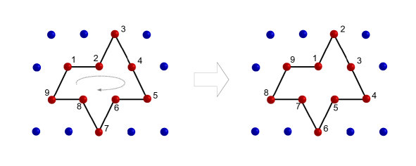
Since the main aim of this paper is to investigate algorithms, we used simple triangular lattice liquid instead of lattice. The lattice of size consists of sites and each lattice site contains one of two types of segments: or . The volume fraction of segment is equal to and for segment it is . The number of each type of segments is constant during simulations so that it is a model with conserved order parameter. An attempt to move a single segment defines a single Monte Carlo step. There are no vacancies on the lattice so that segments can move via cooperative motion in which a few elements are moved at the same time, as shown in fig. 1. This single cooperative motion is called a cooperative loop. Figure 1a presents a single loop before segments are moved and the final state is presented in fig. 1b. In the athermal state (without interaction between segments) this cooperative loop is created in the following way:
-
1.
a segment from random lattice site is removed (temporary vacancy is created) and this site is labeled both INITIAL and CURRENT,
-
2.
one of six neighbors of CURRENT lattice site is selected at random,
-
3.
segment from this selected site is moved to CURRENT site and selected site becomes the CURRENT one,
-
4.
points 2 and 3 are iterated until the random neighbor is not the same as the INITIAL site,
-
5.
the segment which was initially removed is put into the vacancy.
After athermal simulation, consisting of such cooperative loops, the segments are randomly distributed on the lattice.
Next, interactions between segments are introduced and described through parameters. The interaction between different type of segment is equal to and between the same type of segment is (). The interaction are limited to nearest neighbors and energy of single segment is ( parameter is also used as energy unit). The reduced temperature is . It means that segments prefer segments of the same type and below the critical temperature, , the system separates in two phases, first is rich in segments and the second in segments .
In case of this thermal simulation various states of system are generated using the same cooperative motions (and also Kawasaki dynamics motions) and probability transition between current state and new state is described by following formula:
| (1) |
In this paper, three approaches employing the Metropolis criterion and also the heuristic method are used.
In the first case, the loop is created using single vacancy which moves as a random walk. The difference of energy is calculated for full loop and , where is energy of the initial state (state before cooperative loop) and is energy of the state after cooperative loop. We use standard Metropolis criteria Metropolis et al. (1953), and refer to this method as , the motions are non-local since more then one segment is moved in a single step of simulation. In this case some mismatch with theory can occur due to possible large energy changes involved with acceptance of long loops, as discussed in next chapter.
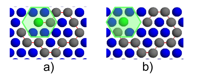
In the second case (), the loop is divided into incremental steps in which the movement of a single segment is analyzed. We refer to it as Metropolis with single vacancy. At the beginning of the loop, the segment from random lattice site is removed without any condition since it decrease energy of system (vacancy which does not interact with segments is created). At the end of the loop, the removed segment is inserted with probability proportional to Boltzmann factor since this motion always increases energy of system. In case of failure, the whole loop is rejected. Inside the loop, describes energy of sliding segment at initial position as shown in fig 2a and describes energy of the same segment at new position (fig. 2b). In a single step, we try to move only one segment.
Moreover, the Metropolis method was employed for the Kawasaki dynamics Kawasaki (1972) (), swapping neighboring lattice sites, which generated results that we use as a background for other methods.
The last approach is similar to method with one exception, the acceptance condition is always based on energy of single segment in new position (energy of previous state is not included in Boltzmann factor). It means that . We call this method as heuristic Monte Carlo method () since the correctness of this approach is not obvious and compare it to commonly used Metropolis criterion can be interesting and provide additional and intriguing insights into CMA algorithm.
We use five different lattice size in presented simulations: , , , , and . First of all, the athermal simulations is performed for at least MCS. Next, we perform thermal run from to MCS depending on lattice size and the first half of run is needed to equilibrate the system, and the second half is used to collect the data. All simulation experiments are repeated at least 3 times starting with different initial athermal states.
In order to improve statistics (particularly at low temperatures) the parallel tempering Earl and Deem (2005); Swendsen and Wang (1986) (PT) algorithm was also used in simulations. In the PT method, replicas of system are simulated in parallel (in this case it was ), each in different temperature , with ranging from to . After a number of Monte Carlo steps (MCS) (in our case it was 500 MCS), we try to exchange replicas with neighboring in random order with the following probability:
| (2) |
where .
III RESULTS AND DISCUSSION
First, we carry out simulations for lattice size equal to . In fig. 3, energy per lattice site, , and heat capacity, in terms of temperature for different methods are presented. The heat capacity is calculated from the equation:
| (3) |
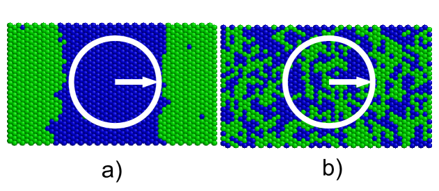
One can observe single peak in at () for all Metropolis approaches as well as heuristic method which is related to the separation of the system into two phases. Above this critical temperatures, , the segments of type and are uniformly distributed on the lattice (like in fig 5b), while below system start to separate into two phases (fig 5a). The first one is rich in segments of type and the second one mostly consists of segments . A significant decrease in energy is observed also at , as shown in fig. 3b. This temperature is consistent with the theoretical value of critical temperature for the Ising model at triangular lattice (with coordination number ) calculated by Houtappel in 1950 Houtappel (1950) and equals to .
In fig. 4a, we present probability of state acceptance, , in term of loop length, , for the method. It is obvious that this probability decreases with loop length increasing and for loop length greater than is close to . We introduces additional parameter that describes contribution of different loop lengths. It determines what length of the loop takes most time of simulation and is described as:
| (4) |
where is the probability of the loop of length . This parameter is shown in fig. 4b. The contribution decreases with loop length increasing and reaches a minimum at about , and then begins to rise sharply. The contribution of short loop length (shorter than ) is significant but the contribution of long loops (greater than ) is more significant. As shown in fig. 4a the probability of acceptance of long loops is close to and this affects the efficiency of method. Since the method is the least efficient, requiring the longest time of simulation, we do not take this approach into account in further analysis.
Moreover, it is possible to determine of the critical temperature with greater precision by calculating the Binder cumulant Binder and Heermann (1992) ():
| (5) |
where is the order parameter described by equation Das et al. (2006):
| (6) |
The is calculated from the histogram of the probability of finding a particle of a given type in a given area. It can be calculated for different temperatures in terms of local concentration of segments type A defined as , where is the number of segment type in specified area and is the total number of segments in the same area. In contrast to the Ising model where the number of spins is not preserved, in presented simulations the volume fraction of segments of different types is constant so can not be calculated for the whole lattice (in that case will be ). In this paper, the radius of this area depends on size of lattice and is equal to as shown in fig. 5. Such approach was previously used and described in ref. Kwak and Landau (2006). The value was chosen arbitrary from a few selected tested values because it provided the best statistics. Moreover, we observed that does not depend on this parameter.
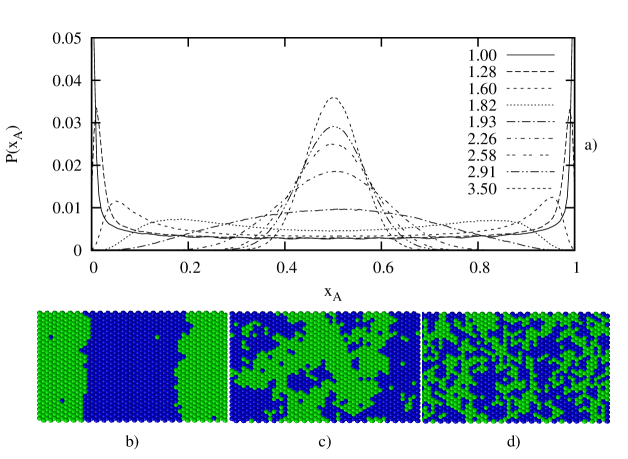
The sample for different temperatures are presented in fig. 6a. For the has Gaussian distribution with maximum at and the peak is getting narrower as the temperature is increased. This means that, statistically, in selected area the same number of segment and is observed (fig. 6d). At system starts to separate into two phases as shown in fig. 6c. Below critical temperature has bimodal distribution with two maxima at and corresponding to two coexisting phases (fig. 6b). Those maxima become narrower with decreasing temperature since the clusters grow and become more homogeneous.
The value of the Binder cumulant depends on size of lattice for different values of temperatures except of where tends towards an universal value and not depending on . For segments are uniformly mixed (system is disordered) and while for system is separated into two phases (ordered) and as shown in fig. 7.
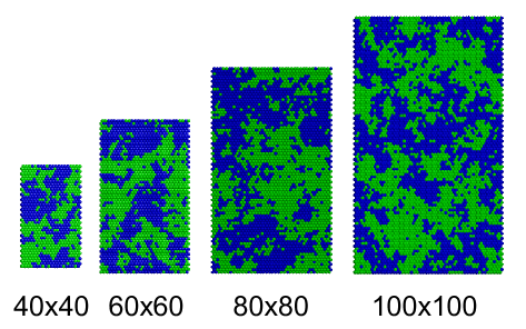
The simulations for different size of lattice were carried out to determine the using the Binder cumulant. We use four values of lattice size: , , , and which are presented in fig. 8. Results of simulations for two Metropolis approaches and heuristic method are presented in fig. 9-11. The summary of the results is presented in table 1. The critical temperatures presented in table 1 are determined on the basis of intersection of the Binder cumulant calculated for different lattice size. We use 48 replicas, different temperatures, in parallel tempering simulations in range form to . The distance between neighboring temperatures is so the simulation error (accuracy of the simulation) is about (). In the case of Kawasaki dynamics which is used as the background for other methods, and the error is . For step acceptance method the average is and the error is . The with error equals to is obtained for method. The critical temperature obtained for heuristic method is consistent with both Metropolis approaches. In all cases the value of error is below the accuracy of the simulation.
IV CONCLUDING REMARKS
We carried out Monte Carlo simulations of simple binary liquid using two methods:
-
•
standard Metropolis (with different approaches),
-
•
heuristic method.
The parameters determined during simulation with different approaches are qualitatively and quantitatively consistent. The critical temperature obtained for all methods is the same with the simulation accuracy. Moreover, the Metropolis with vacancy as well as heuristic method (where loops are divided into incremental steps) are more efficient than standard Metropolis method with full loop acceptance what is important for the simulation of dense polymer system.
Acknowledgements.
P.K. and M.B. gratefully acknowledge the research grant from the Polish NCN No. DEC-2012/07/N/ST4/00293 and the computational grant from the Supercomputing and Networking Center (PSNC) in Poznan, Poland.References
- Frenkel and Smit (2001) D. Frenkel and B. Smit, Understanding Molecular Simulation, Second Edition: From Algorithms to Applications (Computational Science) (Academic Press, 2001).
- Metropolis et al. (1953) N. Metropolis, A. Rosenbluth, M. Rosenbluth, A. Teller, and E. Teller, Journal of Chemical Physics 21, 1087 (1953).
- Binder (1997) K. Binder, Reports on Progress in Physics 60, 487 (1997).
- Newman and Barkema (1999) M. E. J. Newman and G. T. Barkema, Monte Carlo Methods in Statistical Physics (Oxford University Press, 1999).
- Fratzl and Penrose (1994) P. Fratzl and O. Penrose, Physical Review B 50, 3477 (1994).
- Halagan and Polanowski (2009) K. Halagan and P. Polanowski, Journal of Non-Crystalline Solids 355, 1318 (2009).
- Kawasaki et al. (1989) K. Kawasaki, T. Nagai, and K. Nakashima, Philosophical Magazine B: Physics of Condensed Matter; Electronic, Optical and Magnetic Properties 60, 399 (1989).
- Yaldram and Binder (1991a) K. Yaldram and K. Binder, Acta Metallurgica Et Materialia 39, 707 (1991a).
- Yaldram and Binder (1991b) K. Yaldram and K. Binder, Journal of Statistical Physics 62, 161 (1991b).
- Pakula (1987) T. Pakula, Macromolecules 20, 679 (1987).
- Pakula and Geyler (1987) T. Pakula and S. Geyler, Macromolecules 20, 2909 (1987).
- Pakula and Geyler (1988) T. Pakula and S. Geyler, Macromolecules 21, 1665 (1988).
- Pakula and Teichmann (1997) T. Pakula and J. Teichmann, Materials Research Society Symposium - Proceedings 455, 211 (1997).
- Gauger et al. (1993a) A. Gauger, A. Weyersberg, and T. Pakula, Macromolecular Theory and Simulations 2, 531 (1993a).
- Weyersberg and Vilgis (1993) A. Weyersberg and T. Vilgis, Physical Review E 48, 377 (1993).
- Gauger et al. (1993b) A. Gauger, A. Weyersberg, and T. Pakula, Die Makromolekulare Chemie, Theory and Simulations 2, 531 (1993b).
- Pakula and Matyjaszewski (1996) T. Pakula and K. Matyjaszewski, Macromolecular Theory and Simulations 5, 987 (1996).
- Pakula et al. (1997) T. Pakula, K. Karatasos, S. H. Anastasiadis, and G. Fytas, Macromolecules 30, 8463 (1997).
- Banaszak et al. (2002) M. Banaszak, S. Wołoszczuk, T. Pakula, and S. Jurga, Physical Review E 66, 031804 (2002).
- Qin et al. (2003) Y. Qin, H.-L. Liu, and Y. Hu, Molecular Simulation 29, 649 (2003).
- Majtyka and Kłos (2006) M. Majtyka and J. Kłos, Journal of Physics Condensed Matter 18, 3581 (2006).
- Jeszka and Pakula (2006) J. Jeszka and T. Pakula, Polymer 47, 7289 (2006).
- Polanowski and Jeszka (2007) P. Polanowski and J. Jeszka, Langmuir 23, 8678 (2007).
- Majtyka and Kłos (2007) M. Majtyka and J. Kłos, Physical Chemistry Chemical Physics 9, 2284 (2007).
- Sikorski et al. (2011) A. Sikorski, P. Polanowski, P. Adamczyk, and S. Zerko, Journal of Molecular Modeling 17, 2209 (2011).
- Polanowski et al. (2013) P. Polanowski, E. Wawrzyńska, and A. Sikorski, Macromolecular Theory and Simulations 22, 238 (2013).
- Knychała et al. (2014) P. Knychała, M. Banaszak, and N. Balsara, Macromolecules 47, 2529 (2014).
- Kawasaki (1972) K. Kawasaki, Phase transitions and critical phenomena, vol. 2 (Academic Press, 1972).
- Earl and Deem (2005) D. J. Earl and M. W. Deem, Physical Chemistry Chemical Physics 7, 3910 (2005).
- Swendsen and Wang (1986) R. H. Swendsen and J. S. Wang, Physical Review Letters 57, 2607 (1986).
- Houtappel (1950) R. Houtappel, Physica 16, 425 (1950).
- Binder and Heermann (1992) K. Binder and D. W. Heermann, Monte Carlo Simulation in Statistical Physics (Springer Verlag, 1992).
- Das et al. (2006) S. Das, J. Horbach, K. Binder, M. Fisher, and J. Sengers, Journal of Chemical Physics 125 (2006).
- Kwak and Landau (2006) W. Kwak and D. Landau, International Journal of Modern Physics C 17, 15 (2006).
| intersection | KA | LM | HE |
| average | |||
| standard deviation | |||
| error |
Figure captions:
Fig. 1: Example of single cooperative motion for triangular lattice. Grey arrow show direction of segment motion.
Fig. 2: Nearest neighbors using to calculate energy of sliding segment (green) before (a) and after (b) move of a single segment.
Fig. 3: Results of simulations (averaged over 5 runs) for lattice size and four different method: (a) heat capacity, , with error bars (b) energy per lattice site, .
Fig. 4: Probability of loop acceptance, , (a) and contribution of different length of loop into simulation, , (b) in term of loop length, , for the method at .
Fig. 5: Size of area (equal to ) which is used in simulation to calculation the density profiles.
Fig. 6: Density profiles for different temperatures (a) and snapshots from simulation for lattice size at (b), (c), (d).
Fig. 7: The sample Binder cumulant in terms of for lattice size .
Fig. 8: Four sizes of box used in simulations to calculate the Binder cumulant.
Fig. 9: The Binder cumulant (average over 3 runs) for the Kawasaki method and four different size of box. The inset shows intersection of the Binder cumulant.
Fig. 10: The Binder cumulant (average over 3 runs) for the method and four different size of box. The inset shows intersection of the Binder cumulant.
Fig. 11: The Binder cumulant (average over 3 runs) for the heuristic method and four different size of box. The inset shows intersection of the Binder cumulant.
