Self-organization and transition to turbulence in isotropic fluid motion driven by negative damping at low wavenumbers

Abstract

We observe a symmetry-breaking transition from a turbulent to a self-organized state in direct numerical simulation of the Navier-Stokes equation at very low Reynolds number. In this self-organised state the kinetic energy is contained only in modes at the lowest resolved wavenumber, the skewness vanishes, and visualization of the flows shows a lack of small-scale structure, with the vorticity and velocity vectors becoming aligned (a Beltrami flow).

One of the better known results in the history of science is the discovery of the laminar-turbulence transition in pipe flow by Osborne Reynolds in the late nineteenth century. Since then such transitions have been found in many other flow configurations, and the subject is widely studied today. In contrast, the commonly accepted view of randomly forced isotropic fluid motion is that the motion is turbulent for all Reynolds numbers and no actual transition to turbulence occurs.

In the course of studying the direct numerical simulation (DNS) of forced isotropic turbulence, we have found that self-organized states form at low Taylor-Reynolds numbers, in simulations which were invariably turbulent at large Taylor-Reynolds numbers, thus hinting at the possibility of a transition to turbulence. We observed depression of the nonlinear term in the Navier-Stokes equation (NSE) during the formation of the self-organized state. Visualization of the flow showed that in the self-organized state the velocity field $\bm{u}$ and vorticity field $\bm{\omega}=\nabla\times\bm{u}$ are aligned in real space, forcing the nonlinear term $\bm{u}\times\bm{\omega}$ in the NSE to vanish. This is known as a Beltrami field Constantin and Majda (1988); Kambe (2010). As it is also a condition for maximum helicity, and the initial state has zero helicity, it follows that the transition to the self-ordered state is symmetry-breaking. Moreover, the flow shows only large-scale structure.

We begin by discussing the details of our ‘numerical experiment’. The incompressible forced NSE was solved numerically, using the standard fully de-aliased pseudospectral method on a 3D periodic domain of length $L_{box}=2\pi$, resulting in the lowest resolved wavenumber $k_{min}=2\pi/L_{box}=1$. We note that our simulation method is both conventional and widely used, so we give only some necessary details here. Full details of our numerical technique and code validation may be found in Yoffe (2012).

We found that a choice of $32^{3}$ collocation points proved to be sufficient in order to resolve the Kolmogorov dissipation scale, as all our simulations in this particular investigation were at very low Reynolds numbers. We did however verify that the formation of the self-organized state was also observed at a higher resolution ($64^{3}$). All simulations were well resolved, satisfying $k_{max}\eta\geqslant 2.16$ McComb et al. (2001), where $\eta$ denotes the Kolmogorov dissipation scale. The maximum time the simulations were evolved for was $t=1000s$, or, in terms of initial large-eddy turnover times $t_{0}=L/U$, $t=1271t_{0}$, where $U$ denotes the initial rms velocity and $L$ the initial integral length scale. Initial Taylor-Reynolds numbers $R_{\lambda}$ ranged from $R_{\lambda}=2.61$ to $R_{\lambda}=3.78$, where $\lambda$ denotes the Taylor microscale. A summary of simulation details is given in Table 1.

$N^{3}$	$k_{max}\eta$	$R_{\lambda,SO}$	$\nu$	$R_{\lambda}$	$t_{max}/s$
$32^{3}$	2.85	12.91	0.1	2.61	1000
$32^{3}$	2.63	15.12	0.09	2.93	1000
$32^{3}$	2.56	15.91	0.087	3.00	1000
$32^{3}$	2.52	16.47	0.085	3.07	1000
$32^{3}$	2.48	17.07	0.083	3.14	1000
$32^{3}$	2.41	18.04	0.08	3.26	1000
$32^{3}$	2.39	18.38	0.079	3.30	1000
$32^{3}$	2.34	19.11	0.077	3.39	1000
$32^{3}$	2.29	19.88	0.075	3.47	1000
$32^{3}$	2.25	20.70	0.073	3.57	1000
$32^{3}$	2.29	21.58	0.071	3.67	1000
$32^{3}$	2.18	22.04	0.07	3.72	1000
$32^{3}$	2.16	22.52	0.069	3.78	1000
$64^{3}$	5.26	15.12	0.09	2.93	1000
$64^{3}$	4.82	18.04	0.08	3.26	1000
$64^{3}$	4.36	22.04	0.07	3.72	1000

Table 1: Specifications of simulations. $N^{3}$ denotes the number of collocation points, $k_{max}$ the largest resolved wavenumber, $\eta$ the Kolmogorov microscale, $R_{\lambda,SO}$ the Taylor-Reynolds number in the self-organized state, $\nu$ the kinematic viscosity, $R_{\lambda}$ the initial Taylor-Reynolds number and $t_{max}$ the time the simulations were evolved for.

The initial conditions were random (Gaussian) velocity fields with prescribed energy spectra of the form

$$E(k)=C_{1}k^{4}e^{-2(k/k_{0})^{2}}\ ,$$ (1)

where $C_{1}=0.001702$ and $k_{0}=5$. The initial helicity $\langle\bm{u}(\bm{k})\bm{\omega}(-\bm{k})\rangle$, where $\bm{\omega}(\bm{k})$ is the Fourier transform of the vorticity field $\bm{\omega}(\bm{x})$, was negligible for all simulations.

The system was forced by negative damping, with the Fourier transform of the force $\bm{f}$ given by

$$\bm{f}(\bm{k},t) =(\varepsilon_{W}/2E_{f})\bm{u}(\bm{k},t)\quad\text{for}\quad 0<\lvert\bm{k}\rvert<k_{f};$$

$$=0\quad\textrm{otherwise},$$ (2)

where $\bm{u}(\bm{k},t)$ is the instantaneous velocity field (in wavenumber space). The highest forced wavenumber, $k_{f}$, was chosen to be $k_{f}=2.5$. As $E_{f}$ was the total energy contained in the forcing band, this ensured that the energy injection rate was $\varepsilon_{W}=\textrm{constant}$.

Negative damping was introduced to turbulence theory by Herring Herring (1965) in 1965 and to DNS by Machiels Machiels (1997) in 1997. Since then it has been used in many different investigations to simulate homogeneous isotropic turbulence (for example, Jiménez et al. (1993); McComb et al. (2001); Yamazaki et al. (2002); Kaneda et al. (2003); McComb and Quinn (2003); McComb et al. (2014, 2015)) and particularly in the benchmark simulations of Kaneda and co-workers Kaneda and Ishihara (2006), with Taylor-Reynolds numbers up to $R_{\lambda}=1200$. It has also been studied theoretically by Doering and Petrov Doering and Petrov (2005).

It should be emphasized that the forcing in the DNS does not relate the force given in (2) to the velocity field in the NSE at the same instant in time. The force added at time $t$ is calculated from the velocity field at the previous time step $t-dt$, where in practice an intermediate predictor-corrector step is taken. This has the important consequence that, because of nonlinear phase mixing during this additional step, the force and the velocity field in the NSE at a given instant in time are not in phase, as long as the nonlinear term is active. Although this forcing procedure does not have an explicit stochastic element, it is nevertheless generally regarded as adding a random force to the fluid. As the velocity field at $t=0$ consists of a (pseudo-)randomly generated set of numbers, the forcing rescales this set of numbers and feeds it back into the system at the first time step; and so on.

In order to investigate aspects of turbulence at high Reynolds number, which are beyond currently available computing power, our invariable practice is to keep $\varepsilon_{W}$ constant, and reduce $\nu$. This corresponds to taking the limit of infinite Reynolds number Batchelor (1953). We have carried out investigations up to $R_{\lambda}=435$ with regards to the behaviour of the dimensionless dissipation rate McComb et al. (2015) and the behavior of the second-order structure function McComb et al. (2014). During these investigations, we observed the peculiar asymptotic behavior of the fluid at low Reynolds numbers as shown in Fig. 1, which was confirmed using the publicly available code hit3d Chumakov (2007, 2008).

At such low Reynolds numbers, we found that initially the simulations developed in the usual way, with clear evidence of nonlinear mixing. But, after long running times, the total energy ceased to fluctuate, and instead remained constant, while the skewness dropped to zero. Once this had happened, the kinetic energy was confined to the $k=1$ mode and the nonlinear transfer had become zero. The cascade process was thus absent and no small-scale structures were being formed. Hence the system had self-organized into a large-scale state.

Similar results were found both with our code and with hit3d as shown in Fig. 1(a). Figure 1(b) shows the evolution of the velocity derivative skewness. Note that it drops to zero at long times, indicating that the observed state is Gaussian and hence is not turbulent. As the velocity derivative skewness is not recorded by hit3d, a comparison using this quantity was not possible.

Since the energy spectrum in the self-organized state is unimodal at $k=1$, we can predict the asymptotic value $E(t)=E_{\infty}$ in this state from the energy input rate $\varepsilon_{W}$ and the viscosity $\nu$ using the spectral energy balance equation for forced isotropic turbulence

$$\frac{\partial E(k,t)}{\partial t}=T(k,t)-2\nu_{0}k^{2}E(k,t)+W(k,t)\ ,$$ (3)

where $E(k,t)$ and $T(k,t)$ are the energy and transfer spectra, respectively, and

$$W(k,t)=4\pi k^{2}\langle\bm{u}(-\bm{k},t)\cdot\bm{f}(\bm{k},t)\rangle$$ (4)

is the work spectrum of the stirring force. By invoking stationarity ($\varepsilon_{W}=\varepsilon$, where $\varepsilon$ denotes the dissipation rate), we obtain for the total energy after self-organization

$$E(t)=E_{\infty}=\frac{\varepsilon_{W}}{2\nu}=\mbox{ constant}\ .$$ (5)

All runs for all values of the initial Taylor-Reynolds number stabilized at this value of $E(t)$. Note that the same value is obtained both with our code and with hit3d as shown in Fig. 1(a). The realisations obtained from hit3d and from our code only differ in the random initial condition while all other parameters such as the viscosity and forcing rate are identical. As can also be seen in Fig. 1(a), although both realisations attain the same asymptotic value of $E(t)$, they do not do so at the same rate.

(a)  Evolution of the total energy

(b)  Evolution of the skewness

Figure 1: Onset of the self-organized state as indicated by the total energy $E(t)$ and the velocity-derivative skewness $S(t)$ for $R_{\lambda}=3.39$. (a) $E(t)$: the solid line shows results from our DNS and the dashed line results from hit3d. Note that the two realisations obtained from the different codes reach the same aysmptotic value of $E(t)$. (b) $S(t)$: evolution of the skewness for the same run. Time is given in units of initial large eddy turnover time $t_{0}=L/U$, where $U$ is the initial rms velocity and $L$ the initial integral scale.

(a)  Transfer spectra at different times for $R_{\lambda}=3.39$.

(b)  Energy spectra at different times for $R_{\lambda}=3.39$.

Figure 2: (a) Transfer spectra at different times showing the depression of nonlinearity as the nonlinear transfer gets weaker as time progresses. The time evolution of the total energy corresponding to the measured spectra is shown in Fig. 1(a). (b) Energy spectra at different times. The formation of a unimodal spectrum in clearly visible. After self-organization only the $k=1$ mode remains populated while all other modes have lost their kinetic energy, where we note that $L\simeq 0.5$. The kinetic energy is therefore concentrated in the large scales and we do not expect small-scale flow patterns. This corresponds to the right-hand image of Fig. 3, where the flow shows only large-scale structure.

The development of the large-scale state was accompanied by a depression of nonlinearity, as shown in Fig. 2(a) where the transfer spectrum $T(k,t)$ is plotted at different times. Again, it should be emphasized that at early times $T(k,t)$ has the behaviour typically found in simulations of isotropic turbulence (see e.g. Fig. 9.3, p. 293 of McComb (2014)), but at later times tends to zero. At the same time, the energy spectrum $E(k,t)$, tends to a unimodal spectrum at $k=1$ as can be seen in Fig. 2(b).

Figure 3 shows snapshots of the system before and after self-organization. The arrows indicate the velocity field $\bm{u}(\bm{x})$ and vorticity field $\bm{\omega}(\bm{x})$ at different points in real space. We may see that the vorticity field and the velocity field align with each other once the system has self-organized, such that

$$\nabla\times\bm{u}(\bm{x})=\bm{\omega}(\bm{x})=\alpha\bm{u}(\bm{x})\ ,$$ (6)

for a coefficient $\alpha$ (which must have dimensions of inverse length). Vector fields satisfying (6) are eigenfunctions of the curl operator and therefore helical. It should be noted that the nonlinear term in the NSE vanishes identically if the velocity and vorticity fields are aligned. From the image on the right hand side of Fig. 3, it can clearly be seen that the flow is in an ordered state, as velocity and vorticity vectors are everywhere parallel to each other, giving visual evidence of the Beltrami property (6) of the large-scale field. Furthermore, we observe a lack of small-scale structure of the flow, which reflects the measured unimodal energy spectrum in the self-organized state. The Beltrami condition has also been verified by analyzing helicity spectra, showing nonzero helicity at $k=1$ and zero helicity at all higher wavenumbers. We found that the final states always satisfied the Beltrami condition. However, final states occur where vorticity and velocity are aligned (positive helicity) or anti-aligned (negative helicity). Which of the two possible helicity states is chosen in the self-organized state depends on the random initial conditions. If a particular final state occurs, then its mirror image will also be a possible asymptotic state that may occur, as there is no systematic preference for a particular configuration.

A short film showing the transition to the self-organized state can be found in the supplemental material (available online at stacks.iop.org/jpa/48/25FT01/mmedia). Two interesting points may be observed from the film. First, the system shows behaviour similar to ‘critical slowing down’ (see e.g. Hohenberg and Halperin (1977)). Secondly, we observe a transition from a non-helical state to a helical state. That is, the formation of the helical self-organized state is symmetry-breaking. This latter aspect can also be seen in Fig. 3.

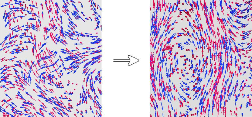
Figure 3: (Color online) Visualization of the velocity field (red arrows) and the vorticity field (blue arrows) in $x$-space before and after self-organization. The alignment between velocity and vorticity fields is clearly visible in the right-hand image. The image shows a slice parallel to the $xy$-plane of the computational domain.

Our results may be peculiar to our particular choice of forcing. We note that as the nonlinear term tends to zero, the phase-mixing also vanishes, and the negative damping becomes in phase with the velocity field. Accordingly there is then no mechanism to restore randomness, and in this simple picture, the self-organized state must be stable. A further implication of this, is that negative damping would be rather difficult to achieve in a real physical system. Accordingly we are currently exploring the effect of other types of forcing and this work will be reported in due course.

However, it is arguable that the combination of the NSE and negative damping is an interesting dynamical system in its own right. For initial values of the Taylor-Reynolds number greater than about $25$ (corresponding to a steady-state value of about $40$), it reproduces isotropic turbulence; while for initial $R_{\lambda}$ less than about 5, it makes a spontaneous, symmetry-breaking transition to a Beltrami state. In the past, there have been mathematical conjectures about the possibility of Beltrami fields Moffatt (1985); Moffatt and Tsinober (1992) (and references therein) in turbulence; and numerical studies have suggested that such fields can occur in a localized way Kraichnan and Panda (1988); Pelz et al. (1985); Kerr (1987). To the best of our knowledge, this present investigation reports the first instance of a spontaneous transition to a stable Beltrami state for an entire flow field.

Furthermore, the emphasis in DNS has always been on achieving ever-larger Reynolds numbers, in order to study asymptotic scaling behaviour. Yet in the case of the dimensionless dissipation, for example, the emphasis is on low Reynolds numbers, and indeed on looking for universal behaviour under these circumstances. Accordingly, the present work also draws attention to the surprising fact that stirred fluid motion at low $R_{\lambda}$ may not actually be turbulent.

One of the few practical applications of isotropic turbulence is in geophysical flows. Our results could possibly be relevant to atmospheric phenomena such as ‘blocking’ Frederiksen (2007), for instance. Recent numerical studies in magnetohydrodynamics show the development of similar organized states Dallas and Alexakis (2015). This suggests a wider relevance of this type of result, not least because it was achieved in a different system using a different forcing scheme from our own.

Investigation into the nature of this transition continues. In view of recent successes of a dynamical systems approach to the transition to turbulence in wall-bounded shear flows, work is currently being carried out taking a similar approach, and this will be submitted for publication in due course.

References

- Constantin and Majda (1988) P. Constantin and A. Majda, Commun. Math. Phys., 115, 435 (1988).
- Kambe (2010) T. Kambe, Geometrical Theory of Dynamical Systems and Fluid Flows, revised ed. (World Scientific, Singapore, 2010).
- Yoffe (2012) S. R. Yoffe, Investigation of the transfer and dissipation of energy in isotropic turbulence, Ph.D. thesis, University of Edinburgh (2012), http://arxiv.org/pdf/1306.3408v1.pdf.
- McComb et al. (2001) W. D. McComb, A. Hunter, and C. Johnston, Phys. Fluids, 13, 2030 (2001).
- Herring (1965) J. R. Herring, Phys. Fluids, 8, 2219 (1965).
- Machiels (1997) L. Machiels, Phys. Rev. Lett., 79, 3411 (1997).
- Jiménez et al. (1993) J. Jiménez, A. A. Wray, P. G. Saffman, and R. S. Rogallo, J. Fluid Mech., 255, 65 (1993).
- Yamazaki et al. (2002) Y. Yamazaki, T. Ishihara, and Y. Kaneda, J. Phys. Soc. Jap., 71, 777 (2002).
- Kaneda et al. (2003) Y. Kaneda, T. Ishihara, M. Yokokawa, K. Itakura, and A. Uno, Phys. Fluids, 15, L21 (2003).
- McComb and Quinn (2003) W. D. McComb and A. P. Quinn, Physica A, 317, 487 (2003).
- McComb et al. (2014) W. D. McComb, S. R. Yoffe, M. F. Linkmann, and A. Berera, Phys. Rev. E, 90, 053010 (2014).
- McComb et al. (2015) W. D. McComb, A. Berera, S. R. Yoffe, and M. F. Linkmann, Phys. Rev. E, 91, 043013 (2015).
- Kaneda and Ishihara (2006) Y. Kaneda and T. Ishihara, Journal of Turbulence, 7, 1 (2006).
- Doering and Petrov (2005) C. R. Doering and N. P. Petrov, “Low-wavenumber forcing and turbulent energy dissipation,” in Progress in Turbulence (Springer Proc. in Physics), Vol. 101, edited by S. B. J. Peincke, A. Kittel and M. Oberlack (Springer, Berlin, 2005) pp. 11–18.
- Batchelor (1953) G. K. Batchelor, The theory of homogeneous turbulence, 1st ed. (Cambridge University Press, Cambridge, 1953).
- Chumakov (2007) S. G. Chumakov, Phys. Fluids, 19, 058104 (2007).
- Chumakov (2008) S. G. Chumakov, Phys. Rev. E, 78, 036313 (2008).
- McComb (2014) W. D. McComb, Homogeneous, Isotropic Turbulence: Phenomenology, Renormalization and Statistical Closures (Oxford University Press, 2014).
- Hohenberg and Halperin (1977) P. C. Hohenberg and B. I. Halperin, Rev. Modern Physics, 49, 435 (1977).
- Moffatt (1985) H. K. Moffatt, J. Fluid Mech., 159, 359 (1985).
- Moffatt and Tsinober (1992) H. K. Moffatt and A. Tsinober, Annu. Rev. Fluid Mech., 24, 281 (1992).
- Kraichnan and Panda (1988) R. H. Kraichnan and R. Panda, Phys. Fluids, 31, 2395 (1988).
- Pelz et al. (1985) R. B. Pelz, V. Yakhot, and S. A. Orszag, Phys. Rev. Lett., 54, 2505 (1985).
- Kerr (1987) R. M. Kerr, Phys. Rev. Lett., 59, 783 (1987).
- Frederiksen (2007) J. S. Frederiksen, in Frontiers in turbulence and coherent structures, edited by J. Denier and J. S. Frederiksen (World Scientific Lecture Notes in Complex Systems, 2007) pp. 29–58.
- Dallas and Alexakis (2015) V. Dallas and A. Alexakis, Phys. Fluids, 27, 045105 (2015).
- (27) http://dx.doi.org/10.7488/ds/250.