Linear Precoding for the MIMO Multiple Access Channel with Finite Alphabet Inputs and
Statistical CSI

Abstract

In this paper, we investigate the design of linear precoders for the multiple-input multiple-output (MIMO) multiple access channel (MAC). We assume that statistical channel state information (CSI) is available at the transmitters and consider the problem under the practical finite alphabet input assumption. First, we derive an asymptotic (in the large system limit) expression for the weighted sum rate (WSR) of the MIMO MAC with finite alphabet inputs and Weichselberger’s MIMO channel model. Subsequently, we obtain the optimal structures of the linear precoders of the users maximizing the asymptotic WSR and an iterative algorithm for determining the precoders. We show that the complexity of the proposed precoder design is significantly lower than that of MIMO MAC precoders designed for finite alphabet inputs and instantaneous CSI. Simulation results for finite alphabet signalling indicate that the proposed precoder achieves significant performance gains over existing precoder designs.

I Introduction

In recent years, the channel capacity and the design of optimum transmission strategies for the multiple-input multiple-output (MIMO) multiple access channel (MAC) have been widely studied [1, 2, 3]. For instance, it was proved in [1] that the boundary of the MIMO MAC capacity region is achieved by Gaussian input signals. It was further demonstrated in [2] that, for the MIMO MAC, the optimization of the transmit signal covariance matrices for weighted sum rate (WSR) maximization leads to a convex optimization problem. For sum rate maximization, the authors of [3] developed an efficient iterative water-filling algorithm for finding the optimal input signal covariance matrices for all users.

However, the results in [1, 2, 3] rely on the critical assumption of Gaussian input signals. Although Gaussian inputs are optimal in theory, they are rarely used in practice. Rather, it is well-known that practical communication signals usually are drawn from finite constellation sets, such as pulse amplitude modulation (PAM), phase shift keying (PSK) modulation, and quadrature amplitude modulation (QAM). These finite constellation sets differ significantly from the Gaussian idealization [4, 5, 6, 7, 8, 9]. Accordingly, transmission schemes designed based on the Gaussian input assumption may result in substantial performance losses when finite alphabet inputs are used for transmission. In [5], the globally optimal linear precoder design for point-to-point communication systems with finite alphabet inputs was obtained, building upon earlier works [10, 11, 12, 13]. For the case of the two-user single-input single-output MAC with finite alphabet inputs, the optimal angle of rotation and the optimal power division between the transmit signals were found in [14] and [15], respectively. For the MIMO MAC with an arbitrary number of users and generic antenna configurations, an iterative algorithm for searching for the optimal precoding matrices of all users was proposed in [6].

The transmission schemes in [5, 6, 7, 8, 9, 10, 11, 12, 13, 14, 15] require accurate instantaneous channel state information (CSI) at the transmitters for precoder design. If the channels vary relatively slowly, in frequency division duplex systems, the instantaneous CSI can be estimated accurately at the receiver via uplink training and then sent to the transmitters through dedicated feedback links, and in time division duplex systems, the instantaneous CSI can be obtained by exploiting the reciprocity of uplink and downlink. Nevertheless, when the mobility of the users increases and channel fluctuations vary more rapidly, the round-trip delays of the CSI become non-negligible with respect to the coherence time of the channels. In this case, the obtained instantaneous CSI at the transmitters might be outdated. Therefore, for these scenarios, it is more reasonable to exploit the channel statistics at the transmitter for precoder design, as the statistics change much more slowly than the instantaneous channel parameters.

Transmitter design for statistical CSI has received much attention for the case of Gaussian input signals [16, 17, 18, 19, 20, 21, 22]. For finite alphabet inputs, point-to-point systems, an efficient precoding algorithm for maximization of the ergodic capacity over Kronecker fading channels was developed in [23]. Also, in [24], asymptotic (in the large system limit) expressions for the mutual information of the MIMO MAC with Kronecker fading were derived. Recently, an iterative algorithm for precoder optimization for sum rate maximization of the MIMO MAC with Kronecker fading was proposed in [25]. Despite these previous works, the study of the MIMO MAC with statistical CSI at the transmitter and finite alphabet inputs remains incomplete, for three reasons: First, the Kronecker fading model characterizes the correlations of the transmit and the receive antennas separately, which is often not in agreement with measurements [26, 27]. In contrast, jointly-correlated fading models, such as Weichselberger’s model [27], do not only account for the correlations at both ends of the link, but also characterize their mutual dependence. As a consequence, Weichselberger’s model provides a more general representation of MIMO channels. Second, explicit structures of the optimal precoders for the MIMO MAC with statistical CSI and finite alphabet inputs have not been reported yet. Third, in contrast to the sum rate, the weighted sum rate (WSR) enables service differentiation in practical communication systems [28]. Thus, it is of interest to study the WSR optimization problem.

In this paper, we investigate the linear precoder design for the $K$-user MIMO MAC assuming Weichselberger’s fading model, finite alphabet inputs, and availability of statistical CSI at the transmitter. By exploiting a random matrix theory tool from statistical physics, referred to as the replica method, we first derive an asymptotic expression for the WSR of the MIMO MAC for Weichselberger’s fading model in the large system regime where the numbers of transmit and receive antennas are both large. The derived expression indicates that the WSR can be obtained asymptotically by calculating the mutual information of each user separately over equivalent deterministic channels. This property significantly reduces the computational effort for calculation of the WSR. Furthermore, we prove that the optimal left singular matrix of each user’s optimal precoder corresponds to the eigenmatrix of the transmit correlation matrix of the user. This result facilitates the derivation of an iterative algorithm for computing the optimal precoder for each user. The proposed algorithm updates the power allocation matrix and the right singular matrix of each user in an alternating manner along the gradient decent direction. We show that the proposed algorithm does not only provide a systematic precoder design method for the MIMO MAC with statistical CSI at the transmitter, but also reduces the implementation complexity by several orders of magnitude compared to the precoder design for instantaneous CSI. Moreover, precoders designed for statistical CSI can be updated much less frequently than precoders designed for instantaneous CSI as the channel statistics change very slowly compared to the instantaneous CSI. Numerical results demonstrate that the proposed design provides substantial performance gains over systems without precoding and systems employing precoders designed under the Gaussian input assumption for both systems with a moderate number of antennas and massive MIMO systems [32].

The remainder of this paper is organized as follows. Section II describes the considered MIMO MAC model. In Section III, we derive the asymptotic mutual information expression for the MIMO MAC with statistical CSI at the transmitter and finite alphabet inputs. In Section IV, we obtain a closed-form expression for the left singular matrix of each user’s precoder maximizing the asymptotic WSR and propose an iterative algorithm for determining the precoders of all users. Numerical results are provided in Section V and our main results are summarized in Section VI.

The following notations are adopted throughout the paper: Column vectors are represented by lower-case bold-face letters, and matrices are represented by upper-case bold-face letters. Superscripts $(\cdot)^{T}$, $(\cdot)^{*}$, and $(\cdot)^{H}$ stand for the matrix/vector transpose, conjugate, and conjugate-transpose operations, respectively. $\rm{det}(\cdot)$ and $\rm{tr}(\cdot)$ denote the matrix determinant and trace operations, respectively. ${\rm{diag}}\left\{\bf{b}\right\}$ and ${\rm{blockdiag}}\left\{{\bf{A}}_{k}\right\}_{k=1}^{K}$ denote a diagonal matrix and a block diagonal matrix containing in the main diagonal and in the block diagonal the elements of vector $\bf{b}$ and matrices ${\bf{A}}_{k},k=1,2,\cdots,K$, respectively. ${\rm{diag}}\left\{\bf{B}\right\}$ denotes a diagonal matrix containing in the main diagonal the diagonal elements of matrix $\mathbf{B}$. $\odot$ and $\bigotimes$ denote the element-wise product and the Kronecker product of two matrices, respectively. ${\rm vec}\left(\mathbf{A}\right)$ is a column vector which contains the stacked columns of matrix $\mathbf{A}$. $[\mathbf{A}]_{mn}$ denotes the element in the $m$th row and $n$th column of matrix $\mathbf{A}$. $\left\|{\mathbf{X}}\right\|_{F}$ denotes the Frobenius norm of matrix $\mathbf{X}$. ${\mathbf{I}}_{M}$ denotes an $M\times M$ identity matrix, and $E_{V}\left[\cdot\right]$ represents the expectation with respect to random variable $V$, which can be a scalar, vector, or matrix. Finally, $D\mathbf{A}$ denotes the integral measure for the real and imaginary parts of the elements of $\mathbf{A}$. That is, for an $n\times m$ matrix $\mathbf{A}$, we have $D\mathbf{A}=\prod_{i=1}^{n}\prod_{j=1}^{m}\frac{d{\rm{Re}}{[\mathbf{A}]_{ij}}d{\rm{Im}}{[\mathbf{A}]_{ij}}}{\pi}$, where $\rm{Re}$ and $\rm{Im}$ extract the real and imaginary parts, respectively.

II System Model

Consider a single-cell MIMO MAC system with $K$ independent users. We suppose each of the $K$ users has $N_{t}$ transmit antennas and the receiver has $N_{r}$ antennas. Then, the received signal $\mathbf{y}\in\mathbb{C}^{N_{r}\times 1}$ is given by

$${\bf{y}}=\sum\limits_{k=1}^{K}{{\bf{H}}_{k}{\bf{x}}_{k}}+{\bf{v}}$$ (1)

where ${\mathbf{x}_{k}}\in\mathbb{C}^{N_{t}\times 1}$ and ${\mathbf{H}}_{k}\in\mathbb{C}^{N_{r}\times N_{t}}$ denote the transmitted signal and the channel matrix of user $k$, respectively. ${\mathbf{v}}\in\mathbb{C}^{N_{r}\times 1}$ is a zero-mean complex Gaussian noise vector with covariance matrix $\mathbf{I}_{N_{r}}$. Furthermore, we make the common assumption (as, e.g., [34, 19]) that the receiver has the instantaneous CSI of all users, and each transmitter has the statistical CSI of all users.

The transmitted signal vector ${\mathbf{x}_{k}}$ can be expressed as

$${\mathbf{x}_{k}}={{\mathbf{B}}_{k}{\mathbf{d}}_{k}}$$ (2)

where ${\mathbf{B}}_{k}\in\mathbb{C}^{N_{t}\times N_{t}}$ and ${\mathbf{d}}_{k}\in\mathbb{C}^{N_{t}\times 1}$ denote the linear precoding matrix and the input data vector of user $k$, respectively. Furthermore, we assume ${\mathbf{d}}_{k}$ is a zero-mean vector with covariance matrix $\mathbf{I}_{N_{t}}$. Instead of employing the traditional assumption of a Gaussian transmit signal, here we assume ${\mathbf{d}}_{k}$ is taken from a discrete constellation, where all elements of the constellation are equally likely. In addition, the transmit signal ${\mathbf{x}_{k}}$ conforms to the power constraint

$$E_{\mathbf{x}_{k}}\left[{\mathbf{x}_{k}^{H}{\mathbf{x}_{k}}}\right]={{\rm{tr}}\left({{\mathbf{B}}_{k}{\mathbf{B}}_{k}^{H}}\right)}\leq P_{k},\ k=1,2,\cdots,K.$$ (3)

For the jointly-correlated fading MIMO channel, we adopt Weichselberger’s model [27] throughout this paper, which is also referred to as the unitary–independent–unitary model [33].  This model jointly characterizes the correlation at the transmitter and receiver side. In particular, for user $k$, $\mathbf{H}_{k}$ is modeled as

$${\bf{H}}_{k}={\bf{U}}_{{\rm{R}}_{k}}\left({{\bf{\widetilde{G}}}_{k}\odot{\bf{W}}_{k}}\right){\bf{U}}_{{\rm{T}}_{k}}^{H}$$ (4)

where ${\bf{U}}_{{\rm{R}}_{k}}=\left[{{\bf{u}}_{{\rm{R}}_{k},1},{\bf{u}}_{{\rm{R}}_{k},2},\cdots,{\bf{u}}_{{\rm{R}}_{k},N_{r}}}\right]\in\mathbb{C}^{N_{r}\times N_{r}}$ and ${\bf{U}}_{{\rm{T}}_{k}}=\left[{{\bf{u}}_{{\rm{T}}_{k},1},{\bf{u}}_{{\rm{T}}_{k},2},\cdots,{\bf{u}}_{{\rm{T}}_{k},N_{t}}}\right]\in\mathbb{C}^{N_{t}\times N_{t}}$ represent deterministic unitary matrices, respectively. ${\bf{\widetilde{G}}}_{k}\in\mathbb{C}^{N_{r}\times N_{t}}$ is a deterministic matrix with real-valued nonnegative elements, and ${\bf{W}}_{k}\in\mathbb{C}^{N_{r}\times N_{t}}$ is a random matrix with independent identically distributed (i.i.d.) Gaussian elements with zero-mean and unit variance. We define ${\bf{G}}_{k}={\bf{\widetilde{{G}}}}_{k}\odot{\bf{\widetilde{{G}}}}_{k}$ and let $g_{k,n,m}$ denote the $(n,m)$th element of matrix ${\bf{G}}_{k}$. Here, $\mathbf{G}_{k}$ is referred to as the “coupling matrix” as $g_{k,n,m}$ corresponds to the average coupling energy between ${\bf{u}}_{{\rm{R}}_{k},n}$ and ${\bf{u}}_{{\rm{T}}_{k},m}$[27]. The transmit and receive correlation matrices of user $k$ can be written as

$$\begin{array}[]{l}{\bf{R}}_{t,k}=E_{{\bf{H}}_{k}}\left[{{\bf{H}}_{k}^{H}{\bf{H}}_{k}}\right]={\bf{U}}_{{\rm{T}}_{k}}\bm{\Gamma}_{{\rm{T}}_{k}}{\bf{U}}_{{\rm{T}}_{k}}^{H}\\ {\bf{R}}_{r,k}=E_{{\bf{H}}_{k}}\left[{{\bf{H}}_{k}{\bf{H}}_{k}^{H}}\right]={\bf{U}}_{{\rm{R}}_{k}}\bm{\Gamma}_{{\rm{R}}_{k}}{\bf{U}}_{{\rm{R}}_{k}}^{H}\\ \end{array}$$ (5)

where $\bm{\Gamma}_{{\rm{T}}_{k}}$ and $\bm{\Gamma}_{{\rm{R}}_{k}}$ are diagonal matrices with main diagonal elements $\left[{{\bf{\Gamma}}_{{\rm{T}}_{k}}}\right]_{mm}=\sum\nolimits_{n=1}^{N_{r}}{g_{k,n,m}}$, $m=1,2,\cdots,N_{t}$, and $\left[{{\bf{\Gamma}}_{{\rm{R}}_{k}}}\right]_{nn}=\sum\nolimits_{m=1}^{N_{t}}{g_{k,n,m}}$, $n=1,2,\cdots,N_{r}$, respectively.

We note that (4) is a general model which includes many popular statistical fading models as special cases. For example, if $\mathbf{G}_{k}$ is a rank-one matrix, then (4) reduces to the separately-correlated Kronecker model [35, 36]. On the other hand, if ${\bf{U}}_{{\rm{R}}_{k}}$ and ${\bf{U}}_{{\rm{T}}_{k}}$ are discrete Fourier transform matrices, (4) corresponds to the virtual channel representation for uniform linear arrays[37].

We emphasize that Weichselberger’s model avoids the separability assumption of the Kronecker model and can account for arbitrary coupling between the transmitter and receiver ends. Therefore, Weichselberger’s model improves the capability to correctly model actual MIMO channels. For example, [27, Fig. 6] shows that Weichselberger’s model can provide significantly more accurate estimates of the mutual information for actual MIMO channels than the Kronecker model. This was the motivation for using Weichselberger’s model in previous work, e.g. [17, 19], and is also the main reason for using it in this paper. Hence, with this flexible model, we can obtain a more accurate theoretical analysis and more realistic performance results for practical communication systems compared to the simple Kronecker model.

III Asymptotic WSR of the MIMO MAC with Finite Alphabet Inputs

We divide all users into two groups, denoted as set $\cal A$ and its complement set ${\cal{A}}^{c}$: ${\cal{A}}=\{i_{1},i_{2},\cdots,i_{K_{1}}\}\subseteq\{1,2,\cdots,K\}$ and ${\cal{A}}^{c}=\{j_{1},j_{2},\cdots,j_{K_{2}}\}$, $K_{1}+K_{2}=K$. Also, we define ${\bf{H}}_{\cal{A}}=\left[{{\bf{H}}_{i_{1}}\ {\bf{H}}_{i_{2}}\cdots\mathbf{H}_{i_{K_{1}}}}\right]$, $\mathbf{d}_{\cal{A}}=\left[\mathbf{d}_{i_{1}}^{T}\ \mathbf{d}_{i_{2}}^{T}\cdots\mathbf{d}_{i_{K_{1}}}^{T}\right]^{T}$, $\mathbf{d}_{{\cal{A}}^{c}}=\left[\mathbf{d}_{j_{1}}^{T}\ \mathbf{d}_{j_{2}}^{T}\cdots\mathbf{d}_{j_{K_{2}}}^{T}\right]^{T}$, $\mathbf{B}_{\cal{A}}={\rm{blockdiag}}\left\{\mathbf{B}_{i_{1}},\mathbf{B}_{i_{2}},\cdots,\mathbf{B}_{i_{K_{1}}}\right\}$, and ${\bf{y}}_{\cal{A}}={\bf{H}}_{\cal{A}}\mathbf{B}_{\cal{A}}\mathbf{d}_{\cal{A}}+{\bf{v}}$. Then, the achievable rate region $(R_{1},R_{2},\cdots,R_{K})$ of the $K$-user MIMO MAC satisfies the following conditions[38]:

$$\sum_{i\in{\cal A}}R_{i}\leq I\left(\mathbf{d}_{\cal A};\mathbf{y}|\mathbf{d}_{{\cal{A}}^{c}}\right),\quad\forall{\cal{A}}\subseteq\{1,2,\cdots,K\}$$ (6)

where

$$I\left({{\bf{d}}_{\cal{A}};{\bf{y}}\left|{{\bf{d}}_{{\cal A}^{c}}}\right.}\right)\!\!=\!\!E_{{\bf{H}}_{\cal{A}}}\!\left[\!{E_{{\bf{d}}_{\cal{A}},{\bf{y}}_{\cal{A}}}\!\left[\!{\log_{2}\frac{{p\left({{\bf{y}}_{\cal{A}}\left|{{\bf{d}}_{\cal{A}}{\bf{,H}}_{\cal{A}}}\right.}\right)}}{{p\left({{\bf{y}}_{\cal{A}}\left|{{\bf{H}}_{\cal{A}}}\right.}\right)}}\left|{\bf{H}}\right._{\cal{A}}}\!\right]}\right].$$ (7)

In (7), ${p}({\bf{y}}_{\cal A}|{\bf{H}}_{\cal A})$ denotes the marginal probability density function (p.d.f.) of $p(\mathbf{d}_{\cal A},\mathbf{y}_{\cal A}|\mathbf{H}_{\cal A})$. As a result, we have

$$I(\mathbf{d}_{\cal A};\mathbf{y}\left|{{\bf{d}}_{{{\cal A}^{c}}}}\right.)=\\ -E_{\mathbf{H}_{\cal A}}\left[E_{\mathbf{y}_{\cal A}}\left[\left.\log_{2}E_{\mathbf{d}_{\cal A}}\left[e^{-\left\|\mathbf{y}_{\cal A}-\mathbf{H}_{\cal A}\mathbf{B}_{\cal A}\mathbf{d}_{\cal A}\right\|^{2}}\right]\right|\mathbf{H}_{\cal A}\right]\right]\\ -N_{r}\log_{2}e.$$ (8)

The expectation in (8) can be evaluated numerically by Monte-Carlo simulation. However, for a large number of antennas, the associated computational complexity could be enormous. Therefore, by employing the replica method, a classical technique from statistical physics, we obtain an asymptotic expression for (8) as detailed in the following.

III-A Some Useful Definitions

We first introduce some useful definitions. Consider a virtual MIMO channel defined by

$$\mathbf{z}_{\cal A}=\sqrt{\mathbf{T}_{\cal A}}\mathbf{B}_{\cal A}\mathbf{d}_{\cal A}+\check{\bf v}_{\cal A}.$$ (9)

Hence, $\mathbf{T}_{\cal A}\in\mathbb{C}^{K_{1}N_{t}\times K_{1}N_{t}}$ is given by $\mathbf{T}_{\cal A}={\rm{blockdiag}}$ $\left\{\mathbf{T}_{i_{1}},\mathbf{T}_{i_{2}},\cdots,\mathbf{T}_{i_{K_{1}}}\right\}\in\mathbb{C}^{K_{1}N_{t}\times K_{1}N_{t}}$, where $\mathbf{T}_{i_{k}}\in\mathbb{C}^{N_{t}\times N_{t}}$ is a deterministic matrix, $k=1,2,\cdots,K_{1}$. $\check{\bf v}_{\cal A}\in\mathbb{C}^{K_{1}N_{r}\times 1}$ is a standard complex Gaussian random vector with i.i.d. elements. The minimum mean square error (MMSE) estimate of signal vector $\mathbf{d}_{\cal A}$ given (9) can be expressed as

$$\hat{\mathbf{d}}_{\cal A}=E_{\mathbf{d}_{\cal A}}\left[\mathbf{d}_{\cal A}\Big{|}\mathbf{z}_{\cal A},\sqrt{\mathbf{T}_{\cal A}},\mathbf{B}_{\cal A}\right].$$ (10)

Define the following mean square error (MSE) matrix

$$\bm{\Omega}_{\cal A}=\mathbf{B}_{\cal A}\mathbf{E}_{\cal A}\mathbf{B}_{\cal A}^{H}$$ (11)

where

$$\mathbf{E}_{\cal A}=E_{\mathbf{z}_{\cal A}}\left[E_{\mathbf{d}_{\cal A}}\left[(\mathbf{d}_{\cal A}-\hat{\mathbf{d}}_{\cal A})(\mathbf{d}_{\cal A}-\hat{\mathbf{d}}_{\cal A})^{H}\right]\right].$$ (12)

Define the matrices of the $i_{k}$th ($i_{1}\leq i_{k}\leq i_{K_{1}}$) user $\bm{\Omega}_{i_{k}}$ and $\bm{E}_{i_{k}}$ as submatrices obtained by extracting the $\left((k-1)N_{t}+1\right)$th to the $(kN_{t})$th row and column elements of matrices $\bm{\Omega}_{\cal A}$ and $\mathbf{E}_{\cal A}$, respectively.

The component matrices $\mathbf{T}_{i_{k}}$ in $\mathbf{T}_{\cal A}$ are functions of auxiliary variables $\{\mathbf{R}_{i_{k}},\bm{\gamma}_{i_{k}},\bm{\psi}_{i_{k}}\}$, which are the solutions of the following set of coupled equations:

$$\left\{\begin{aligned} \mathbf{T}_{i_{k}}&=\mathbf{U}_{{\rm T}_{i_{k}}}{\rm diag}\left(\mathbf{G}_{i_{k}}^{T}\bm{\gamma}_{i_{k}}\right)\mathbf{U}_{{\rm T}_{i_{k}}}^{H}\in\mathbb{C}^{N_{t}\times N_{t}}\\ \mathbf{R}_{i_{k}}&=\mathbf{U}_{{\rm R}_{i_{k}}}{\rm diag}\left(\mathbf{G}_{i_{k}}\bm{\psi}_{i_{k}}\right)\mathbf{U}_{{\rm R}_{i_{k}}}^{H}\in\mathbb{C}^{N_{r}\times N_{r}}\end{aligned}\right.$$ (13)

where $\bm{\gamma}_{i_{k}}=[\gamma_{i_{k},1},\gamma_{i_{k},2},\cdots,\gamma_{i_{k},N_{r}}]^{T}$ and $\bm{\psi}_{i_{k}}=[\psi_{i_{k},1},\psi_{i_{k},2},\cdots,\psi_{i_{k},N_{t}}]^{T}$ with

$$\left\{\begin{aligned} \gamma_{i_{k},n}&=\mathbf{u}_{{\rm R}_{i_{k}},n}^{H}\left(\mathbf{I}_{N_{r}}+\mathbf{R}_{\cal A}\right)^{-1}\mathbf{u}_{{\rm R}_{i_{k}},n},\ n=1,2,\cdots,N_{r}\\ \psi_{i_{k},m}&=\mathbf{u}_{{\rm T}_{i_{k}},m}^{H}\mathbf{\Omega}_{i_{k}}\mathbf{u}_{{\rm T}_{i_{k}},m},\ m=1,2,\cdots,N_{t}\end{aligned}\right.$$ (14)

and $\mathbf{R}_{\cal A}=\sum_{k=1}^{K_{1}}\mathbf{R}_{i_{k}}$. Computing $\mathbf{T}_{i_{k}}$ requires finding $\{\mathbf{R}_{i_{k}},\bm{\gamma}_{i_{k}},\bm{\psi}_{i_{k}}\}$ through fixed point equations (13) and (14). We will show later that in the asymptotic regime the mutual information in (8) can be evaluated based on the virtual MIMO channel in (9). However, in contrast to channel matrix $\mathbf{H}_{\cal A}$ in (8), for the virtual MIMO channel, channel matrix $\sqrt{\mathbf{T}_{\cal A}}$ is deterministic.

III-B Asymptotic Mutual Information

Suppose the transmit signal ${\mathbf{d}}_{k}$ is taken from a discrete constellation with cardinality $Q_{k}$. Define $M_{k}={Q_{k}^{N_{t}}}$, let ${\cal{S}}_{k}$ denote the constellation set for user $k$, and let ${\mathbf{a}}_{k,j}$ denote the $j$th element of ${\cal{S}}_{k}$, $k=1,2,\cdots,K$, $j=1,2,\cdots,M_{k}$. We define the large system limit as the scenario where $N_{r}$ and $N_{t}$ are large but the ratio $\beta=N_{t}/N_{r}$ is fixed. Now, we are ready to provide a simplified asymptotic expression for (8).

Proposition 1

For the MIMO MAC model (1), in the large system limit the mutual information in (8) can be asymptotically approximated by

$$I\left({{\bf{d}}_{\cal A};{\bf{y}}\left|{{\bf{d}}_{{{\cal A}^{c}}}}\right.}\right)\simeq\sum\limits_{i\in\cal A}{I\left({{\bf{d}}_{i_{k}};{\bf{z}}_{i_{k}}\left|{\sqrt{{\bf{T}}_{i_{k}}}{\bf{B}}_{i_{k}}}\right.}\right)}\\ +\log_{2}\det\left(\mathbf{I}_{N_{r}}+\mathbf{R}_{\cal A}\right)-\log_{2}e\sum_{k=1}^{K_{1}}\bm{\gamma}_{i_{k}}^{T}\mathbf{G}_{i_{k}}\bm{\psi}_{i_{k}}$$ (15)

where

$$I\left({{\bf{d}}_{i_{k}};{\bf{z}}_{i_{k}}\left|{\sqrt{{\bf{T}}_{i_{k}}}{\bf{B}}_{i_{k}}}\right.}\right)=\log_{2}M_{i_{k}}-\frac{1}{{M_{i_{k}}}}\\ \times\sum\limits_{m=1}^{M_{i_{k}}}{E_{{\bf{v}}}\!\left\{\!{\log_{2}\sum\limits_{p=1}^{M_{i_{k}}}{e^{-\left({\left\|{\sqrt{{\bf{T}}_{i_{k}}}{\bf{B}}_{i_{k}}\left({{\bf{a}}_{k,p}\!-\!{\bf{a}}_{k,m}}\right)+{\bf{v}}}\right\|^{2}-\left\|{{\bf{v}}}\right\|^{2}}\right)}}}\!\right\}}.$$ (16)

Proof:

See Appendix A. ∎

Remark 1: The asymptotic expressions provided in Proposition 1 constitute approximations for matrices of finite dimension. In addition, because the derivation of the asymptotic expression is based on the replica method, wherein some steps lack a rigorous proof, we state the result in a proposition rather than a theorem.

Remark 2: As mentioned above, Weichselberger’s model is a general channel model. Therefore, the unified expression in Proposition 1 is applicable to many special cases. For example, if $\mathbf{G}_{k}$ is a rank-one matrix, (15) reduces to [25, Eq. (28)], which was derived for the Kronecker model.

Remark 3: $\bm{\gamma}_{i_{k}}$ and $\bm{\psi}_{i_{k}}$ in Proposition 1 can be obtained through the fixed-point equations in (14). From statistical physics, it is known that there are multiple solutions for $\gamma_{i_{k},n}$ and $\psi_{i_{k},m}$ that satisfy (14). For the problem at hand, the solution minimizing $I\left({{\bf{d}}_{\cal A};{\bf{y}}\left|{{\bf{d}}_{{{\cal A}^{c}}}}\right.}\right)$ in (15) yields the mutual information.

Before proceeding, let us recall some notations used in this paper. For the virtual channel model (9), the virtual channel matrix and the corresponding asymptotic parameters obtained for different sets ${\cal A}$ based on the fixed point equations (13) and (14) are different due to the equality $\mathbf{R}_{\cal A}=\sum_{i_{k}\in{\cal A}}\mathbf{R}_{i_{k}}$. Therefore, we define the set ${\cal A}_{k}=\left\{1,2,\cdots,k\right\}$. Then, we denote the virtual channel matrix and the corresponding asymptotic parameters obtained from the fixed point equations (13) and (14), (9), and (11) for ${\cal{A}}={\cal A}_{k}$ as $\mathbf{T}^{(k)}_{t}$, $\mathbf{R}^{(k)}_{t}$, ${\bm{\gamma}}^{(k)}_{t}$, ${\bm{\psi}}^{(k)}_{t}$, ${\bf{z}}_{t}^{\left(k\right)}$, ${\bm{E}}^{(k)}_{t}$, and ${\bm{\Omega}}^{(k)}_{t}$, $t=1,2,\cdots,k$. Here, the indices $[i_{1},i_{2},\cdots,i_{K_{1}}]$ in (13) and (14) are $[1,2,\cdots,k]$, and $t$ refers to the individual users in the set $[1,2,\cdots,k]$.

IV Linear Precoding Design for the MIMO MAC

In this section, we first formulate the WSR optimization problem for linear precoder design for the MIMO MAC. Then, we establish the structure of the asymptotically optimal precoders maximizing the WSR in the large system limit. Finally, we propose an iterative algorithm for finding the optimal precoders.

IV-A Weighted Asymptotic Sum Rate

It is well known that the achievable rate region of the MIMO MAC $(R_{1},R_{2},\cdots,R_{K})$ can be obtained by solving the WSR optimization problem [1]. Without loss of generality, assume weights $\mu_{1}\geq\mu_{2}\geq\cdots\geq\mu_{K}\geq\mu_{K+1}=0$, i.e., the users are decoded in the order $K,K-1,\cdots,1$ [6]. Then, the WSR problem can be expressed as

$${{\rm WSR}}=\mathop{\max}\limits_{{\mathbf{B}_{1},\mathbf{B}_{2},\cdots,\mathbf{B}_{K}}} ~{}~{}R_{\rm sum}^{{\rm w}}(\mathbf{B}_{1},\mathbf{B}_{2},\cdots,\mathbf{B}_{K}),$$ (17)

s.t. $$~{}~{}\text{tr}\left(\mathbf{B}_{k}\mathbf{B}^{H}_{k}\right)\leq P_{k},~{}\forall k$$

where

$$R_{\rm sum}^{{\rm w}}(\mathbf{B}_{1},\mathbf{B}_{2},\cdots,\mathbf{B}_{K})=\sum\limits_{k=1}^{K}\Delta_{k}f(\mathbf{B}_{1},\mathbf{B}_{2},\cdots,\mathbf{B}_{k})$$ (18)

with $\Delta_{k}=\mu_{k}-\mu_{k+1}$ and $f(\mathbf{B}_{1},\mathbf{B}_{2},\cdots,\mathbf{B}_{k})=I(\mathbf{d}_{1},\cdots,\mathbf{d}_{k};\mathbf{y}|\mathbf{d}_{k+1},\cdots,\mathbf{d}_{K})$, $k=1,2,\cdots,K$. By evaluating $I(\mathbf{d}_{1},\cdots,\mathbf{d}_{k};\mathbf{y}|\mathbf{d}_{k+1},\cdots,\mathbf{d}_{K})$ based on Proposition 1, we obtain an asymptotic expression $R_{\rm sum,asy}^{{\rm w}}(\mathbf{B}_{1},\mathbf{B}_{2},\cdots,\mathbf{B}_{K})$ for $R_{\rm sum}^{{\rm w}}(\mathbf{B}_{1},\mathbf{B}_{2},\cdots,\mathbf{B}_{K})$ in (17). When $\mu_{1}=\mu_{2}=\cdots=\mu_{K}=1$, (17) reduces to the sum rate maximization.

IV-B Asymptotically Optimal Precoder Structure

Consider the singular value decomposition (SVD) of the precoder of user $l$, $\mathbf{B}_{l}=\mathbf{U}_{{\rm B}_{l}}\mathbf{\Gamma}_{{\rm B}_{l}}\mathbf{V}_{{\rm B}_{l}}$, where $\mathbf{U}_{{\rm B}_{l}}$ and $\mathbf{V}_{{\rm B}_{l}}$ are unitary matrices, and $\mathbf{\Gamma}_{{\rm B}_{l}}$ is a diagonal matrix with non-negative main diagonal elements. Then, we have the following theorem.

Theorem 1

The left singular matrices $\mathbf{U}_{{\rm B}_{l}}$ of the asymptotically optimal precoders which maximize the asymptotic WSR $R_{\rm sum,asy}^{{\rm w}}\left({\mathbf{B}}_{1},{\mathbf{B}}_{2},\cdots,{\mathbf{B}}_{K}\right)$ are the eigenmatrices $\mathbf{U}_{{\rm T}_{l}}$ of the transmit correlation matrices in (5), $l=1,2,\cdots,K$. Using the new notations below Remark 3 and based on the optimal precoder structure, (17) simplifies to

$$\max_{\mathbf{\Gamma}_{{\rm B}_{l}},\mathbf{V}_{{\rm B}_{l}},\atop{\text{tr}\left(\mathbf{\Gamma}_{{\rm B}_{l}}^{2}\right)\leq P_{l}}}~{}\sum\limits_{k=l}^{K}{{\Delta_{k}}I\left({{{\bf{d}}_{l}};{\bf{z}}_{l}^{\left(k\right)}\left|{\sqrt{{\rm diag}\left({{\bf{G}}_{l}^{T}{\bm{\gamma}}_{l}^{\left(k\right)}}\right)}\mathbf{\Gamma}_{{\rm B}_{l}}\mathbf{V}_{{\rm B}_{l}}}\right.}\right)}$$ (19)

for $l=1,2,\cdots,K$.

Proof:

See Appendix B. ∎

Remark 4: We note that for finite alphabet input scenarios, the optimal precoder structure of the left singular matrix has been obtained for point-to-point MIMO systems [5, 23]. Also, the optimal precoder structure for the MIMO MAC was implicitly used in [25] for the Kronecker model and finite alphabet inputs without proof. Therefore, the main contribution of Theorem 1 is the explicit presentation of the optimal precoder structure for the MIMO MAC for Weichselberger’s model and finite alphabet inputs and its proof.

Remark 5: For Weichselberger’s model in (4), if only sum rate maximization is considered, i.e., $\Delta_{1}=\Delta_{2}$ $=\cdots=\Delta_{K-1}$, we can directly optimize matrix $\mathbf{V}_{{\rm B}_{L}}^{H}\mathbf{\Gamma}_{{\rm B}_{L}}^{H}{{\rm diag}\left({{\bf{G}}_{L}^{T}{\color[rgb]{0,0,0}\bm{\gamma}}_{L}^{\left(k\right)}}\right)}\mathbf{\Gamma}_{{\rm B}_{L}}\mathbf{V}_{{\rm B}_{L}}$ [25] since the mutual information expression in (19) is concave with respect to this matrix. However, for WSR optimization, since the values of ${\color[rgb]{0,0,0}\bm{\gamma}}_{l}^{\left(k\right)}$ are different for different $k$, it is not possible to find a common matrix $\mathbf{V}_{{\rm B}_{l}}^{H}\mathbf{\Gamma}_{{\rm B}_{l}}^{H}{{\rm diag}\left({{\bf{G}}_{l}^{T}{\color[rgb]{0,0,0}\bm{\gamma}}_{l}^{\left(k\right)}}\right)}\mathbf{\Gamma}_{{\rm B}_{l}}\mathbf{V}_{{\rm B}_{l}}$ to be optimized in (19). Thus, we optimize $\mathbf{\Gamma}_{{\rm B}_{l}}$ and $\mathbf{V}_{{\rm B}_{l}}$ in an alternating manner.

Algorithm 1

Iterative algorithm for WSR maximization with respect to $\left\{{\mathbf{B}}_{1},{\mathbf{B}}_{2},\cdots,{\mathbf{B}}_{K}\right\}$  

1. Initialize $\mathbf{\Gamma}_{{\rm B}_{l}}^{(1)}$, $\mathbf{V}_{{\rm B}_{l}}^{(1)}$, $l=1,2,\cdots,K$, ${\bf{T}}^{(k)}_{t}$, ${\bf{R}}^{(k)}_{t}$, ${\bm{\psi}}_{t}^{(k),\left({{1}}\right)}$, and ${\bm{\gamma}}_{t}^{(k),\left({{1}}\right)}$, $t=1,2,\cdots,k$, $k=1,2,\cdots,K$. Set $n=1$ and compute $R_{\rm sum,asy}^{{{\rm w}},(n)}$.

2. Update $\left({\mathbf{\Gamma}}_{{\rm B}_{l}}^{(n+1)}\right)^{2}$, $l=1,2,\cdots,K$, along the gradient decent direction in (20).

3. Update $\mathbf{V}_{{\rm B}_{l}}^{(n+1)}$, $l=1,2,\cdots,K$, along the gradient decent direction in (21).

4. Compute ${\mathbf{B}}_{l}^{(n+1)}=\mathbf{U}_{{\rm T}_{l}}\mathbf{\Gamma}_{{\rm B}_{l}}^{(n+1)}\mathbf{V}_{{\rm B}_{l}}^{(n+1)}$ and update the asymptotic parameters ${\bf{T}}^{(k)}_{t}$, ${\bf{R}}^{(k)}_{t}$, ${\bm{\gamma}}_{t}^{(k),\left({{n+1}}\right)}$, and ${\bm{\psi}}_{t}^{(k),\left({{n+1}}\right)}$.

5. Compute $R_{\rm sum,asy}^{{{\rm w}},(n+1)}$. If $R_{\rm sum,asy}^{{{\rm w}},(n+1)}-R_{\rm sum,asy}^{{{\rm w}},(n)}$ is larger than a threshold and $n$ is less than the maximal number of iterations, set $n:=n+1$, repeat Steps $2$–$4$; otherwise, stop the algorithm.

    

Next, we obtain the gradients of $R_{\rm sum,asy}^{\color[rgb]{0,0,0}\rm w}\left({\mathbf{B}}_{1},{\mathbf{B}}_{2},\right.$ $\left.\cdots,{\mathbf{B}}_{K}\right)$ with respect to $\mathbf{\Gamma}_{{\rm B}_{l}}^{2}$ and $\mathbf{V}_{{\rm B}_{l}}$, which are given by [5, Eq. (19)] and [40, Eq. (22)] as

$${\nabla_{{\bf{\Gamma}}_{{{\rm{B}}_{l}}}^{2}}}R_{{\rm{sum,asy}}}^{\rm{w}}\left({{{\bf{B}}_{1}},{{\bf{B}}_{2}},\cdots,{{\bf{B}}_{K}}}\right)\\ =\sum\limits_{k=l}^{K}{{\Delta_{k}}{\rm{diag}}\left({{\bf{V}}_{{{\rm{B}}_{l}}}^{H}{\bf{E}}_{l}^{\left(k\right)}{{\bf{V}}_{{{\rm{B}}_{l}}}}{\rm{diag}}\left({{\bf{G}}_{l}^{T}{\color[rgb]{0,0,0}\bm{\gamma}}_{l}^{\left(k\right)}}\right)}\right)}$$ (20)

and

$${\nabla_{{{\bf{V}}_{{{\rm{B}}_{l}}}}}}R_{{\rm{sum,asy}}}^{\rm{w}}\left({{{\bf{B}}_{1}},{{\bf{B}}_{2}},\cdots,{{\bf{B}}_{K}}}\right)\\ =\sum\limits_{k=l}^{K}{{\Delta_{k}}{\rm{diag}}\left({{\bf{G}}_{l}^{T}{\color[rgb]{0,0,0}\bm{\gamma}}_{l}^{\left(k\right)}}\right){\bf{\Gamma}}_{{{\rm{B}}_{l}}}^{2}}{{\bf{V}}_{{{\rm{B}}_{l}}}}{\bf{E}}_{l}^{\left(k\right)},$$ (21)

respectively. Now, we are ready to propose an iterative algorithm to determine the optimal precoders $\mathbf{B}_{l}$ numerically.

IV-C Iterative Algorithm for Weighted Sum Rate Maximization

Based on Theorem 1, (20), and (21), an efficient iterative algorithm can be formulated to determine the optimal precoders $\mathbf{B}_{l}$ numerically. The resulting algorithm is summarized in Algorithm 1.

In Step 2 of Algorithm 1, we optimize $\left(\mathbf{\Gamma}_{{\rm B}_{l}}^{(n)}\right)^{2}$ along the gradient descent direction $\left(\widetilde{\mathbf{\Gamma}}_{{\rm B}_{l}}^{(n)}\right)^{2}=$ $\left(\mathbf{\Gamma}_{{\rm B}_{l}}^{(n)}\right)^{2}+u{\nabla_{{\bf{\Gamma}}_{{{\rm{B}}_{l}}}^{2}}}R_{{\rm{sum,asy}}}^{\rm{w}}\left({{{\bf{B}}_{1}},{{\bf{B}}_{2}},\cdots,{{\bf{B}}_{K}}}\right)$, where ${\nabla_{{\bf{\Gamma}}_{{{\rm{B}}_{l}}}^{2}}}R_{{\rm{sum,asy}}}^{\rm{w}}\left({{{\bf{B}}_{1}},{{\bf{B}}_{2}},\cdots,{{\bf{B}}_{K}}}\right)$ is given by (20) and the step size $u$ is determined by the backtracking line search method [42]. Thereby, the values of the backtracking line search parameters $\theta$ and $\omega$ are set as $\theta\in(0,0.5)$ and $\omega\in(0,1)$ [42]. If the updated $\left(\widetilde{\mathbf{\Gamma}}_{{\rm B}_{l}}^{(n)}\right)^{2}$ has negative elements, we set those to zero, normalize $\left(\widetilde{\mathbf{\Gamma}}_{{\rm B}_{l}}^{(n)}\right)^{2}$ [25], and then update $\left({\mathbf{\Gamma}}_{{\rm B}_{l}}^{(n+1)}\right)^{2}=\left(\widetilde{\mathbf{\Gamma}}_{{\rm B}_{l}}^{(n)}\right)^{2}$. In Step 3, we optimize $\mathbf{V}_{{\rm B}_{l}}^{(n)}$ along the gradient descent direction $\widetilde{\mathbf{V}}_{{\rm B}_{l}}^{(n)}=\mathbf{V}_{{\rm B}_{l}}^{(n)}+u{\nabla_{{\bf{V}}_{{{\rm{B}}_{l}}}}}R_{{\rm{sum,asy}}}^{\rm{w}}\left({{{\bf{B}}_{1}},{{\bf{B}}_{2}},\cdots,{{\bf{B}}_{K}}}\right)$, where ${\nabla_{{\bf{V}}_{{{\rm{B}}_{l}}}}}R_{{\rm{sum,asy}}}^{\rm{w}}\left({{{\bf{B}}_{1}},{{\bf{B}}_{2}},\cdots,{{\bf{B}}_{K}}}\right)$ is given by (21). We compute the SVD of $\widetilde{\mathbf{V}}_{{\rm B}_{l}}^{(n)}=\mathbf{U}_{{\rm{V}}_{l}}\mathbf{\Gamma}_{{\rm V}_{l}}\mathbf{V}_{{\rm V}_{l}}$. Then, we project $\widetilde{\mathbf{V}}_{{\rm B}_{l}}^{(n)}$ on the Stiefel manifold ${\mathbf{V}}_{{\rm B}_{l}}^{(n+1)}=\mathbf{U}_{{\rm{V}}_{l}}\mathbf{V}_{{\rm V}_{l}}$ [41, Sec. 7.4.8]. In Step 4, we compute ${\mathbf{B}}_{l}^{(n+1)}=\mathbf{U}_{{\rm T}_{l}}\mathbf{\Gamma}_{{\rm B}_{l}}^{(n+1)}\mathbf{V}_{{\rm B}_{l}}^{(n+1)}$. Then, we update the asymptotic parameters ${\bf{T}}^{(k)}_{t}$, ${\bf{R}}^{(k)}_{t}$, ${\bm{\gamma}}_{t}^{(k),\left({{n+1}}\right)}$, and ${\bm{\psi}}_{t}^{(k),\left({{n+1}}\right)}$ in Proposition 1 based on the updated precoders ${\bf{B}}_{l}^{\left(n+1\right)}$, $l=1,2,\cdots,K$, and the fixed point equations (13) and (14). In Step 5, we compute $R_{\rm sum,asy}^{{{\rm w}},(n+1)}$ based on ${\mathbf{B}}_{l}^{(n+1)}$, $l=1,2,\cdots,K$, ${\bf{T}}^{(k)}_{t}$, ${\bf{R}}^{(k)}_{t}$, ${\bm{\gamma}}_{t}^{(k),\left({{n+1}}\right)}$, and ${\bm{\psi}}_{t}^{(k),\left({{n+1}}\right)}$, $t=1,2,\cdots,k$, $k=1,2,\cdots,K$. Finally, if $R_{\rm sum,asy}^{{{\rm w}},(n+1)}-R_{\rm sum,asy}^{{{\rm w}},(n)}$ is larger than a threshold and $n$ is less than the maximal number of iterations, we perform the next iteration, otherwise, we stop the algorithm.

Remark 6: We note that the iterative algorithms in [5] and [23] are for point-to-point MIMO systems. Therefore, both algorithms only need to consider the maximization of a single mutual information expression. For the MIMO MAC, the iterative algorithm in [6] optimizes the precoders of all users jointly. Therefore, its implementation complexity is very high. Based on the asymptotic WSR expression, Algorithm 1 optimizes the precoder of each user separately. Thus, its implementation complexity is significantly lower than that of the iterative algorithm in [6]. Moreover, Algorithm 1 exploits the optimal structure of the precoders for WSR maximization and optimizes the power allocation matrix and the right singular matrix of the precoder of each user in an alternating manner. The iterative algorithm in [25] is for the Kronecker model. For the special case of the Kronecker model, even for WSR optimization, ${\bm{\gamma}}_{l}^{\left(k\right)}$ can be moved outside $\mathbf{V}_{{\rm B}_{l}}^{H}\mathbf{\Gamma}_{{\rm B}_{l}}^{H}{{\rm diag}\left({{\bf{G}}_{l}^{T}{\bm{\gamma}}_{l}^{\left(k\right)}}\right)}$ $\mathbf{\Gamma}_{{\rm B}_{l}}\mathbf{V}_{{\rm B}_{l}}$, as indicated in [25]. Hence, for the Kronecker model, the algorithm in [25] can also be used to optimize the WSR and may be preferable for numerical calculation. This is because the algorithm in [25] only requires an eigenvalue decomposition where Algorithm 1 requires a SVD. However, as indicated in Remark 5, the algorithm in [25] can not be directly applied to the WSR optimization problem for Weichselberger’s model considered in this paper.

Remark 7: We note that calculating the mutual information and the MSE matrix (e.g., (16), (20), (21) or [6, Eq. (5)], [6, Eq. (24)]) involves additions over the modulation signal space which scales exponentially with the number of transmit antennas. The computational complexity of other operations, such as the matrix product, solving the fixed point equations, etc., are polynomial functions of the number of transmit and receive antennas. Therefore, for ease of analysis, we just compare the computational complexity of calculating the mutual information and the MSE matrix here. When $N_{t}$ increases, the computational complexity of Algorithm 1 is dominated by the required number of additions in calculating $R_{\rm sum,asy}^{{\color[rgb]{0,0,0}\rm w},(n)}\left({\mathbf{B}}_{1},{\mathbf{B}}_{2},\cdots,{\mathbf{B}}_{K}\right)$, ${\nabla_{{\bf{\Gamma}}_{{{\rm{B}}_{l}}}^{2}}}R_{{\rm{sum,asy}}}^{\rm{w}}\left({{{\bf{B}}_{1}},{{\bf{B}}_{2}},\cdots,{{\bf{B}}_{K}}}\right)$, and ${\nabla_{{\bf{V}}_{{{\rm{B}}_{l}}}}}R_{{\rm{sum,asy}}}^{\rm{w}}$ $\left({{{\bf{B}}_{1}},{{\bf{B}}_{2}}},\cdots,{{{\bf{B}}_{K}}}\right)$ based on (16) in Steps 1 and 5, Step 2, and Step 3, respectively. Eq. (16) implies that Algorithm 1 only requires additions over each user’s own possible transmit vectors to design the precoders. Accordingly, the computational complexity of the proposed Algorithm 1 in calculating the mutual information and the MSE matrix grows linearly with $\sum\nolimits_{k=1}^{K}{Q_{k}^{2N_{t}}}$. In contrast, the conventional precoder design for instantaneous CSI at the transmitter in [6] requires additions over all possible transmit vectors of all users. For this reason, the computational complexity of the conventional precoding design scales linearly with $\left({\prod\nolimits_{k=1}^{K}{Q_{k}}}\right)^{2N_{t}}$. As a result, the computational complexity of Algorithm 1 is significantly lower than that of the conventional design. We note that this computational complexity reduction is more obvious when the number of transmit antennas or the number of users become large.

To show this more clearly, we give an example. We consider a practical massive MIMO MAC system where the base station is equipped with a large number of antennas and serves multiple users having much smaller numbers of antennas [32, 43, 44, 45, 46, 47]. In particular, we assume $N_{r}=64$, $N_{t}=4$, $K=4$, $\mu_{1}=\mu_{2}=\mu_{3}=\mu_{4}$, and all users employ the same modulation constellation. The numbers of additions required for calculating the mutual information and the MSE matrix in Algorithm 1 and in the precoder design in [6] are listed in Table I for different modulation formats.

TABLE I: Number of additions required for calculating the mutual information and the MSE matrix.

Modulation	QPSK	8PSK	16 QAM
Algorithm 1	262144	6.7 e+007	1.7 e+010
Design Method in [6]	1.85 e+019	7.9 e+028	3.4 e+038

We observe from Table I that Algorithm 1 requires a significantly lower number of additions for the MIMO MAC precoder design for finite alphabet inputs compared to the design in [6]. Moreover, since Algorithm 1 is based on the channel statistics $\{\mathbf{U}_{{\rm T}_{k}}\}_{\forall k}$, $\{\mathbf{U}_{{\rm R}_{k}}\}_{\forall k}$, $\{\mathbf{G}_{k}\}_{\forall k}$, it avoids the time-consuming averaging process over each channel realization of the mutual information in (7). In addition, Algorithm 1 is executed only once since the precoders are constant as long as the channel statistics do not change, whereas the algorithm in [6] has to be executed for each channel realization.

Remark 8: We note that Algorithm 1 never decreases the asymptotic WSR $R_{\rm sum,asy}^{\rm w}\left({\mathbf{B}}_{1},{\mathbf{B}}_{2},\cdots,{\mathbf{B}}_{K}\right)$ in any iteration, see Step 5. From the expression in (15), we also know that the asymptotic WSR $R_{\rm sum,asy}^{\rm w}\left({\mathbf{B}}_{1},{\mathbf{B}}_{2},\cdots,{\mathbf{B}}_{K}\right)$ is upper-bounded. This implies that Algorithm 1, which produces non-decreasing sequences that are upper-bounded, is convergent. Due to the non-convexity of the objective function $R_{\rm sum,asy}^{\color[rgb]{0,0,0}\rm w}\left({\mathbf{B}}_{1},{\mathbf{B}}_{2},\cdots,{\mathbf{B}}_{K}\right)$, in general, Algorithm 1 will find a local maximum of the WSR. Therefore, we run Algorithm 1 for several random initializations ${\mathbf{B}}_{k}^{(1)}$ and select the result that offers the maximal WSR as the final design solution [6, 48].

V Numerical Results

In this section, we provide examples to illustrate the performance of the proposed iterative optimization algorithm. We assume equal individual power limits $P_{1}=P_{2}=\cdots=P_{K}=P$ and the same modulation format for all $K$ users. The average SNR for the MIMO MAC with statistical CSI is defined as ${\rm{SNR}}=\frac{{E\left[{{{\rm{tr}}\left({{\bf{H}}_{k}{\bf{H}}_{k}^{H}}\right)}}\right]P}}{{N_{t}N_{r}}}$. We use GP, NP, FAP, and AL as abbreviations for Gaussian precoding, no precoding, finite alphabet precoding, and algorithm in [6], respectively.

First, we consider a two-user MIMO MAC with two transmit antennas for each user and two receive antennas in order to illustrate that, although Algorithm 1 was derived for the large system limit, it also performs well if the numbers of antennas are small. For the channel statistics of Weichselberger’s model, ${\bf{U}}_{{\rm{T}}_{k}}$, ${\bf{U}}_{{\rm{R}}_{k}}$, and ${{\bf\widetilde{G}}_{k}}$, $k=1,2$, are chosen at random.

Figure 1 depicts the average exact sum rate obtained based on (8) and the sum rate obtained with the asymptotic expression in Proposition 1 for different precoding designs and QPSK inputs. For the case without precoding, we set ${\mathbf{B}}_{1}={\mathbf{B}}_{2}=\sqrt{\frac{P}{N_{t}}}\mathbf{I}_{N_{t}}$, and denote the corresponding exact and asymptotic sum rates as “NP, Exact” and “NP, Asymptotic”, respectively. Furthermore, we denote the exact and asymptotic sum rates achieved by the design proposed in Algorithm 1 as “FAP, Exact” and “FAP, Asympotic”. From Figure 1, we observe that the asymptotic sum rate expression in Proposition 1 provides a good estimate of the exact sum rate even for small numbers of antennas. On the other hand, if the numbers of antennas are large, evaluating the exact mutual information in (7) numerically via Monte Carlo simulation is extremely time-consuming. In contrast, Proposition 1 provides an efficient method for estimating the ergodic WSR of the MIMO MAC with finite alphabet inputs.

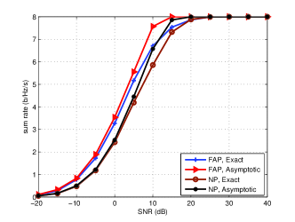
Figure 1: Average sum rate for different precoding designs.

Figure 2 illustrates the convergence behavior of Algorithm 1 for different SNR values and QPSK inputs. We set the backtracking line search parameters to $\theta=0.1$ and $\omega=0.5$. Figure 2 shows the sum rate in each iteration. We observe that in all considered cases, the proposed algorithm needs only a few iterations to converge.

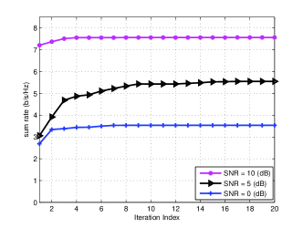
Figure 2: Sum rate vs. iteration index for different SNRs, QPSK inputs, $\theta=0.1$, and $\omega=0.5$.

In Figure 3, we show the sum rate for different transmission schemes and QPSK inputs. We employ the Gauss-Seidel algorithm together with stochastic programming to obtain the optimal covariance matrices of the users under the Gaussian input assumption [19]. Then, we decompose the obtained optimal covariance matrices $\left\{{{\mathbf{Q}}_{1},{\mathbf{Q}}_{2},\cdots,{\mathbf{Q}}_{K}}\right\}$ as ${\mathbf{Q}}_{k}={\mathbf{U}}_{k}\bm{\Lambda}_{k}{\mathbf{U}}_{k}^{H}$, and set ${\mathbf{B}}_{k}={\mathbf{U}}_{k}\bm{\Lambda}_{k}^{\frac{1}{2}}$, $k=1,2,\cdots,K$. Finally, we calculate the average sum rate for this precoding design for QPSK inputs. We denote the corresponding sum rate as “GP with QPSK inputs”. For the case without precoding, we set ${\mathbf{B}}_{1}={\mathbf{B}}_{2}=\sqrt{\frac{P}{N_{t}}}\mathbf{I}_{N_{t}}$. We denote the corresponding sum rate as “NP with QPSK inputs”. We denote the proposed design in Algorithm 1 as “FAP with QPSK inputs”. For comparison purpose, we also show the average sum rate achieved by Algorithm 1 in [6] with instantaneous CSI and denote it as “AL in [12] with QPSK inputs”. The sum rates achieved with the Gauss-Seidel algorithm and without precoding for Gaussian inputs are also plotted in Figure 3, and are denoted as “GP with Gaussian input” and “NP with Gaussian input”, respectively.

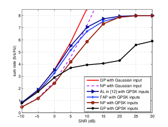
Figure 3: Average sum rate of two-user MIMO MAC with QPSK modulation.

From Figure 3, we make the following observations: 1) For QPSK modulation, the proposed iterative algorithm achieves a considerably higher sum rate compared to the other statistical CSI based precoder designs. Specifically, to achieve a target sum rate of $4$ b/s/Hz, the proposed algorithm achieves SNR gains of approximately $2.5$ dB and $11$ dB compared to the “NP with QPSK inputs” design and the “GP with QPSK inputs” design, respectively. 2) The sum rate achieved by the proposed algorithm is close to the sum rate achieved by Algorithm 1 in [6] which requires instantaneous CSI. At a target sum rate of $4$ b/s/Hz, the SNR gap between the proposed algorithm and Algorithm 1 in [6] is less than 1 dB. However, the proposed algorithm only requires statistical CSI and its implementation complexity is much lower than that of Algorithm 1 in [6]. 3) The sum rate achieved by the proposed algorithm and the “NP with QPSK inputs” design merge at high SNR, and both saturate at $K\log_{2}M=8$ b/s/Hz. 4) The sum rate achieved by the “GP with QPSK inputs” design remains almost constant for SNRs between $10$ dB and $20$ dB. This is because the Gauss-Seidel algorithm design implements a “water filling” power allocation policy in this SNR region. As a result, when the SNR is smaller than a threshold (e.g., 20 dB in this case), the precoders allocate most of the available power to the strongest subchannels and allocate little power to the weaker subchannels. Therefore, one eigenvalue of ${\mathbf{Q}}_{k}$ approaches zero. For example, for $\rm{SNR}=10$ dB, the optimal covariance matrices obtained by the Gauss-Seidel algorithm are given by

$${\mathbf{Q}}_{1} = \left[\begin{array}[]{l}1.2599\qquad\qquad\quad\ 0.9619+0.0790j\\ 0.9619-0.0790j\quad 0.7401\\ \end{array}\right]$$ (24)

$${\mathbf{Q}}_{2} = \left[\begin{array}[]{l}\ \ \,0.1495\qquad\qquad\qquad-0.5214+0.0651j\\ -0.5214-0.0651j\qquad\ \ 1.8505\\ \end{array}\right].$$ (27)

After eigenvalue decomposition ${\mathbf{Q}}_{k}={\mathbf{U}}_{k}\bm{\Lambda}_{k}{\mathbf{U}}_{k}^{H}$, we have

$$\bm{\Lambda}_{1} = \rm{diag}\left\{9.9976,0.0024\right\},$$

$$\bm{\Lambda}_{2} = \rm{diag}\left\{9.9987,0.0013\right\}.$$ (29)

The precoders are given by

$${\mathbf{B}}_{1}=\left[\begin{array}[]{l}-2.5097-0.0000j\qquad 0.0298-0.0000j\\ -1.9168+0.1574j\quad-0.0388+0.0032j\\ \end{array}\right]$$ (32)

$${\mathbf{B}}_{2}=\left[\begin{array}[]{l}-0.8638+0.0000j\quad-0.0349-0.0000j\\ \ \ 3.0184+0.3767j\quad\ -0.0098-0.0012j\\ \end{array}\right].$$ (35)

From the structure of the precoders in (32), we can see that most energy is allocated to one transmitted symbol. For finite alphabet inputs, this power allocation policy may result in allocating most power to the subchannels that are close to saturation. This will lead to a waste of transmit power and impede the further improvement of the sum rate performance. This confirms that precoders designed under the ideal Gaussian input assumption may result in a considerable performance loss when adopted directly in practical systems with finite alphabet constraints.

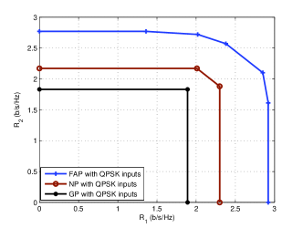
Figure 4: Achivable rate regions of two-user MIMO MAC with QPSK modulation.

In Figure 4, we show the achievable rate region of different precoder designs for ${\rm SNR}=5$ dB and QPSK inputs. The achievable rate regions are obtained by solving the WSR optimization problem in (17) for different precoder designs. We observe from Figure 4 that the proposed design has a much larger rate region than the case without precoding and the design based on the Gaussian input assumption. We note that since for GP, most energy is allocated to one transmitted symbol, for finite alphabet inputs, the achievable sum rate of this transmission design may result in a value that is even smaller than the single user rate. Therefore, there is only one point in the achievable rate region for the GP design. A similar phenomenon has also been observed for the MIMO MAC with instantaneous CSI and finite alphabet inputs, see [6, Fig. 6].

To further validate the performance of the proposed design, Figure 5 shows the sum rate performance for different precoding schemes for 16QAM modulation. Figure 5 indicates that the proposed design outperforms the other precoding schemes also for 16QAM modulation. At a sum rate of $8$ b/s/Hz, the proposed algorithm achieves SNR gains of about $1.7$ dB and $7.5$ dB over the “NP with 16QAM inputs” design and the “GP with 16QAM inputs” design, respectively.

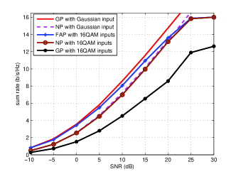
Figure 5: Average sum rate of two-user MIMO MAC with 16QAM modulation.

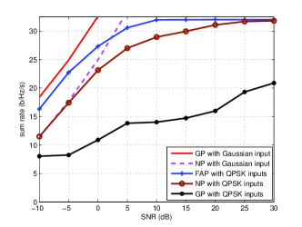
Figure 6: Average sum rate of four-user massive MIMO MAC in suburban scenario with QPSK modulation.

In the following, we investigate the performance of the proposed precoder design in a practical massive MIMO MAC system where the base station is equipped with a large number of antennas and simultaneously serves multiple users with much smaller numbers of antennas [32, 43, 44, 45]. We assume $N_{r}=64$ and $N_{t}=4$. Furthermore, we adopt the 3rd generation partnership project spatial channel model (SCM) in [49]. We set the transmit and receive antenna spacings to half a wave length, and the velocity of the users to $180$ km/h. Figures 6 and 7 show the sum rate performance for different precoder designs, $K=4$, and QPSK inputs for the suburban and the urban scenarios of the SCM, respectively. We observe from Figures 6 and 7 that, for QPSK inputs, the proposed algorithm achieves a better performance than the other precoder designs for both scenarios. For a sum rate of $24$ b/s/Hz, the SNR gains of the proposed algorithm over the “NP with QPSK inputs” design for the suburban and the urban scenarios are about $5$ dB and $4.5$ dB, respectively. The SNR gain for the suburban scenarios is larger than that for the urban scenarios, since the correlation of the transmit antennas is stronger in suburban scenarios. As a result, the precoder design based on statistical CSI is more effective and yields a larger performance gain. Also, the “GP with QPSK inputs” design results in a substantial performance loss in both scenarios. To illustrate the importance of designing the precoders for Weichsenberger’s channel model, we also show in Figure 7 the sum rate performance of precoders designed for the Kronecker’s model (i.e., the mutual coupling is ignored for precoder calculation) and denote the corresponding curve as “FAP with QPSK inputs and KR”. We observe from Figure 7 that for a sum rate of $24$ b/s/Hz, we lose about $1$ dB in performance if we design the precoders for the Kronecker’s model.

Figure 8 shows the average sum rate for different precoder designs as a function of the number of users for QPSK inputs, the urban scenario, and $\rm{SNR}=0$ dB. We observe from Figure 8 that the average sum rate scales linearly with the number of users. This coincides with the conclusion in Proposition 1 that the sum rate can be approximated by the sum of the individual rates of all users.

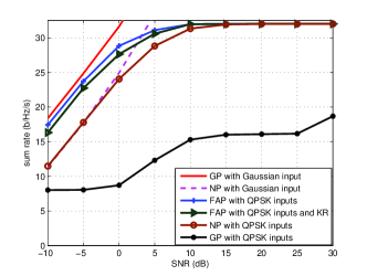
Figure 7: Average sum rate of four-user massive MIMO MAC in urban scenario with QPSK modulation.

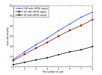
Figure 8: Average sum rate of massive MIMO MAC in urban scenario with QPSK modulation.

VI Conclusion

In this paper, we have studied the linear precoder design for the $K$-user MIMO MAC with statistical CSI at the transmitter. We formulated the problem from the standpoint of finite alphabet inputs based on Weichselberger’s MIMO channel model. We first obtained the WSR expression for the MIMO MAC assuming Weichselberger’s model for the asymptotic large system regime under the finite alphabet input constraint. Then, we established the optimal structures of the precoding matrices which maximize the asymptotic WSR. Subsequently, we proposed an iterative algorithm to find the precoding matrices of all users for statistical CSI at the transmitter. We show that the proposed algorithm significantly reduces the implementation complexity compared to a previously proposed precoder design method for the MIMO MAC with finite alphabet inputs and instantaneous CSI at the transmitter. Numerical results showed that, for finite alphabet inputs, precoders designed with the proposed iterative algorithm achieve substantial performance gains over precoders designed based on the Gaussian input assumption and transmission without precoding. These gains can be observed for both MIMO systems with small numbers of antennas and massive MIMO systems.

Appendix A Proof of Proposition 1

Before we present the proof, we introduce the following three useful lemmas.

Lemma 1

Let $\mathbf{S}\in\mathbb{C}^{m\times n}$, $\mathbf{A}_{1}\in\mathbb{C}^{m\times n}$, and $\mathbf{A}_{2}\in\mathbb{C}^{m\times n}$ be complex matrices and $\mathbf{A}_{3}\in\mathbb{C}^{n\times n}$ and $\mathbf{A}_{4}\in\mathbb{C}^{m\times m}$ positive definite matrices, respectively. Then, the following equality holds [39]:

$$\int D\mathbf{S}\,e^{-{\text{tr}}\left(\mathbf{A}_{3}\mathbf{S}^{H}\mathbf{A}_{4}\mathbf{S}+\mathbf{A}_{1}^{H}\mathbf{S}-\mathbf{S}^{H}\mathbf{A}_{2}\right)}\\ =\frac{1}{\det(\mathbf{A}_{3}\otimes\mathbf{A}_{4})}e^{-{\text{tr}}\left(\mathbf{A}_{3}^{-1}\mathbf{A}_{1}^{H}\mathbf{A}_{4}^{-1}\mathbf{A}_{2}\right)}.$$ (36)

For $\mathbf{A}_{1}=\mathbf{A}_{2}={\bf 0}$ and Gaussian random matrix $\mathbf{S}$, we obtain with this lemma the useful result

$$\int D\mathbf{S}\,e^{-{\sf tr}\left(\mathbf{A}_{3}\mathbf{S}^{H}\mathbf{A}_{4}\mathbf{S}\right)}=\frac{1}{\det(\mathbf{A}_{3}\otimes\mathbf{A}_{4})}.$$ (37)

Lemma 2

The eigen-decomposition of matrix ${\bf A}=b{\bf 11}^{H}+(a-b)\mathbf{I}_{r+1}\in{\mathbb{C}}^{(r+1)\times(r+1)}$, where ${\bf{1}}\in\mathbb{C}^{(r+1)\times 1}$ is the all-one vector, and $a$ and $b$ are arbitrary constants, is

$${\bf A}={\bf F}\ {\rm diag}\left(a+rb,a-b,\cdots,a-b\right){\bf F}^{H}$$ (38)

where $\mathbf{F}\in{\mathbb{C}}^{(r+1)\times 1}$ is the discrete Fourier transform matrix with elements $[{\bf F}]_{nm}=\frac{1}{\sqrt{r+1}}e^{-j\frac{2\pi}{r+1}(n-1)(m-1)}$.

Lemma 3

Hubbard-Stratonovich Transformation: Let ${\bf s}$ and ${\bf a}$ be arbitrary $m\times 1$ complex vectors. Then, we have

$$e^{{\bf a}^{\dagger}{\bf a}}=\int D{\bf s}e^{-({\bf s}^{\dagger}{\bf s}-{\bf a}^{\dagger}{\bf s}-{\bf s}^{\dagger}{\bf a})}.$$ (39)

The identity can be proven easily by using the definition of a matrix variate Gaussian distribution. The transformation is a convenient tool to reduce a quadratic form to a linear expression by introducing auxiliary variables [51].

Now, we begin with the proof of Proposition 1. We note that throughout this section, the virtual channel model defined in Section III-A is only used if explicitly stated. First, we consider the case $K_{1}=K$. Define ${\bf{H}}=\left[{{\bf{H}}_{1}\ {\bf{H}}_{2}\cdots\mathbf{H}_{{K}}}\right]$, $\mathbf{B}={\rm{blockdiag}}\left\{\mathbf{B}_{1},\mathbf{B}_{2},\cdots,\right.$ $\left.\mathbf{B}_{K}\right\}$, $\mathbf{x}=\left[\mathbf{x}_{1}^{T}\ \mathbf{x}_{2}^{T}\cdots\mathbf{x}_{K}^{T}\right]^{T}$, and $\mathbf{d}=\left[\mathbf{d}_{1}^{T}\ \mathbf{d}_{2}^{T}\cdots\mathbf{d}_{K}^{T}\right]^{T}$. From (8), the mutual information of the MIMO MAC can be expressed as $I(\mathbf{d};{\bf y})=F-N_{r}\log_{2}e$, where $F=-{E}_{{\bf y},\mathbf{H}}\left[\log_{2}Z({\bf y},\mathbf{H})\right]$ and $Z({\bf y},\mathbf{H})={E}_{\mathbf{x}}\left[e^{-\left\|{\bf y}-\mathbf{Hx}\right\|^{2}}\right]$. The expectations over $\mathbf{y}$ and $\mathbf{H}$ are difficult to perform because the logarithm appears inside the average. The replica method [50] circumvents this difficulty by rewriting $F$ as

$$F=-\log_{2}e\lim_{r\rightarrow 0}\frac{\partial}{\partial r}\ln{E}_{{\bf y},\mathbf{H}}\left[\left(Z({\bf y},\mathbf{H})\right)^{r}\right].$$ (40)

This reformulation is very useful because it allows us to first evaluate ${E}_{{\bf y},\mathbf{H}}\left[\left(Z({\bf y},\mathbf{H})\right)^{r}\right]$ for a positive integer-valued $r$, and then extend the result to $r\rightarrow 0$. Note, however, that the replica method is not rigorous. Nevertheless, it has been widely adopted in the field of statistical physics [51] and has been also used to derive a number of interesting results in information and communication theory [24, 29, 30, 31, 19, 39, 54]. Some results obtained based on the replica method have been recently confirmed by more rigorous analyses, see e.g. [52, 53].

In a first step, to compute the expectation over $Z({\bf y},\mathbf{H})$, it is useful to introduce $r+1$ replicated signal vectors $\mathbf{x}_{k}^{(\alpha)}$, for $\alpha=0,1,\cdots,r$, yielding

$${E}_{{\bf y},\mathbf{H}}\left[\left(Z({\bf y},\mathbf{H})\right)^{r}\right]\!=\!{E}_{\mathbf{H},\mathbf{X}}\left[\int D\mathbf{y}\prod_{\alpha=0}^{r}e^{-\left\|{\bf y}-\sum_{k=1}^{K}\mathbf{H}_{k}\mathbf{x}_{k}^{(\alpha)}\right\|^{2}}\right]$$ (41)

where $\mathbf{X}=\left[\mathbf{X}_{1}^{T}\,\mathbf{X}_{2}^{T}\,\cdots\,\mathbf{X}_{K}^{T}\right]^{T}$, $\mathbf{X}_{k}=\left[\mathbf{x}_{k}^{(0)}\,\mathbf{x}_{k}^{(1)}\,\cdots\,\mathbf{x}_{k}^{(r)}\right]$, and the $\{\mathbf{x}_{k}^{(\alpha)}\}$ are i.i.d. with distribution $p(\mathbf{x}_{k})$. Now, the integration over $\mathbf{y}$ can be performed in (41) because it is reduced to the Gaussian integral. However, the expectations over $\mathbf{H}$ and $\mathbf{X}$ are involved. To tackle this problem, we separate the expectations with respect to $\mathbf{X}$ and $\mathbf{H}$. Towards this end, define a set of random matrices: $\mathbf{V}=\left[\mathbf{V}_{1}\,\mathbf{V}_{2}\,\cdots\,\mathbf{V}_{K}\right]$, $\mathbf{V}_{k}=\left[\mathbf{v}_{k,1}^{T}\,\mathbf{v}_{k,2}^{T}\,\cdots\mathbf{v}_{k,N_{r}}^{T}\right]^{T}$ and random vectors $\mathbf{v}_{k,n}=\sum_{m}\mathbf{v}_{k,n,m}$, $\mathbf{v}_{k,n,m}=\left[v_{k,n,m}^{(0)}\,v_{k,n,m}^{(1)}\,\cdots\,v_{k,n,m}^{(r)}\right]$, and $v_{k,n,m}^{(\alpha)}=[\mathbf{W}_{k}]_{n,m}[\tilde{\mathbf{G}}_{k}]_{n,m}\mathbf{u}_{{\rm T}_{k},m}^{H}$ $\mathbf{x}_{k}^{(\alpha)}$ for $\alpha=0,1,\cdots,r$. Then, we have from (4)

$$\mathbf{H}_{k}\mathbf{x}_{k}^{(\alpha)}=\sum_{n=1}^{N_{r}}\left(\sum_{m=1}^{N_{t}}v_{k,n,m}^{(\alpha)}\right)\mathbf{u}_{{\rm R}_{k},n}.$$ (42)

Notice that, for given $\mathbf{X}_{k}$, $\mathbf{v}_{k,n,m}$ is a Gaussian random vector with zero mean and covariance matrix $\mathbf{Q}_{k,n,m}$, where $\mathbf{Q}_{k,n,m}\in{\mathbb{C}}^{(r+1)\times(r+1)}$ is a matrix with entries $[\mathbf{Q}_{k,n,m}]_{\alpha\beta}={E}_{[\mathbf{W}_{k}]_{n,m}}\left[\left(v_{k,n,m}^{(\alpha)}\right)^{H}v_{k,n,m}^{(\beta)}\right]=g_{k,n,m}\left(\mathbf{x}_{k}^{(\alpha)}\right)^{H}\mathbf{u}_{{\rm T}_{k},m}\mathbf{u}_{{\rm T}_{k},m}^{H}\mathbf{x}_{k}^{(\beta)}$ for $\alpha=0,1,\cdots,r$, $\beta=0,1,\cdots,r$. For ease of notation, we further define $\mathbf{T}_{k,m}=\mathbf{u}_{{\rm T}_{k},m}\mathbf{u}_{{\rm T}_{k},m}^{H}$ and $\mathbf{R}_{k,n}=\mathbf{u}_{{\rm R}_{k},n}\mathbf{u}_{{\rm R}_{k},n}^{H}$. Therefore, we have $[\mathbf{Q}_{k,n,m}]_{\alpha\beta}=g_{k,n,m}\left(\mathbf{x}_{k}^{(\alpha)}\right)^{H}\mathbf{T}_{k,m}\mathbf{x}_{k}^{(\beta)}$. Using (42) and letting ${\mathbb{Q}}=\{\mathbf{Q}_{k,n,m}\}_{\forall k,n,m}$, where ${\forall k,n,m}$ stands for $k=1,2,\cdots,K$, $m=1,2,\cdots,N_{t}$, and $n=1,2,\cdots,N_{r}$, we have

$${E}_{\mathbf{H}}\left[\int D\mathbf{y}\prod_{\alpha=0}^{r}e^{-\left\|{\bf y}-\sum_{k=1}^{K}\mathbf{H}_{k}\mathbf{x}_{k}^{(\alpha)}\right\|^{2}}\right]=e^{\mathcal{S}({\mathbb{Q}})}$$ (43)

where

$$\mathcal{S}({\mathbb{Q}})=\ln\int D\mathbf{y}\\ \times{E}_{\mathbf{V}}\left[\!\prod_{\alpha=0}^{r}e^{-\left\|{\bf y}-\sum_{k=1}^{K}\left(\sum_{n=1}^{N_{r}}\left(\sum_{m=1}^{N_{t}}v_{k,n,m}^{(\alpha)}\right)\mathbf{u}_{{\rm R}_{k},n}\right)\right\|^{2}}\right].$$ (44)

Clearly, the interactions between $\mathbf{H}$ and $\mathbf{X}$ depend only on ${\mathbb{Q}}$. Therefore, it is useful to separate the expectation over $\mathbf{X}$ in (41) into an integral over all possible $\mathbf{Q}_{k,n,m}$ and all possible $\mathbf{x}_{k}^{(\alpha)}$ configurations for a given $\mathbf{Q}_{k,n,m}$ by introducing a $\delta$-function,

$${E}_{{\bf y},\mathbf{H}}\left[\left(Z({\bf y},\mathbf{H})\right)^{r}\right]=\\ {E}_{\mathbf{X}}\left[\int\prod_{k,n,m}\prod_{0\leq\alpha\leq\beta}^{r}d[\mathbf{Q}_{k,n,m}]_{\alpha\beta}\,e^{\mathcal{S}({\mathbb{Q}})}\right.\\ \times\prod_{k,n,m}\prod_{0\leq\alpha\leq\beta}^{r}\delta\left(g_{k,n,m}\left(\mathbf{x}_{k}^{(\alpha)}\right)^{H}\mathbf{T}_{k,m}\mathbf{x}_{k}^{(\beta)}\right.\\ \left.\left.-[\mathbf{Q}_{k,n,m}]_{\alpha\beta}\vphantom{g_{k,n,m}\left(\mathbf{x}_{k}^{(\alpha)}\right)^{H}\mathbf{T}_{k,m}\mathbf{x}_{k}^{(\beta)}}\right)\vphantom{\int\prod_{k,n,m}}\right].$$ (45)

Let

$$\mu({\mathbb{Q}})={E}_{\mathbf{X}}\left[\prod_{k,n,m}\prod_{0\leq\alpha\leq\beta}^{r}\delta\left(g_{k,n,m}\left(\mathbf{x}_{k}^{(\alpha)}\right)^{H}\mathbf{T}_{k,m}\mathbf{x}_{k}^{(\beta)}\right.\right.\\ \left.\left.-[\mathbf{Q}_{k,n,m}]_{\alpha\beta}\vphantom{g_{k,n,m}\left(\mathbf{x}_{k}^{(\alpha)}\right)^{H}\mathbf{T}_{k,m}\mathbf{x}_{k}^{(\beta)}}\right)\vphantom{\prod_{k,n,m}\prod_{0\leq\alpha\leq\beta}^{r}}\right].$$ (46)

Clearly, (45) can be written as

$${E}_{{\bf y},\mathbf{H}}\left[\left(Z({\bf y},\mathbf{H})\right)^{r}\right]=\int e^{\mathcal{S}({\mathbb{Q}})}d\mu({\mathbb{Q}}).$$ (47)

Now, integrating the function in (45) over ${\bf y}$, (44) becomes

$$e^{\mathcal{S}({\mathbb{Q}})}={E}_{\mathbf{V}}\left[\frac{1}{(r+1)^{N}}e^{-{\rm tr}\left(\left(\sum_{k}(\mathbf{U}_{{\rm R}_{k}}\mathbf{V}_{k})\right){\bf\Sigma}\left(\sum_{k}(\mathbf{U}_{{\rm R}_{k}}\mathbf{V}_{k})\right)^{H}\right)}\right]$$ (48)

where ${\bf\Sigma}=-\frac{1}{(r+1)}{\bf 1}{\bf 1}^{H}+\mathbf{I}_{r+1}$. Recalling that $\mathbf{v}_{k,n,m}$ is a zero-mean Gaussian vector with covariance matrix $\mathbf{Q}_{k,n,m}$, we obtain that $\sum_{k}(\mathbf{U}_{{\rm R}_{k}}\mathbf{V}_{k})$ is a zero-mean Gaussian random vector with covariance $\mathbf{Q}\otimes\mathbf{R}=\sum_{k,n}\left(\sum_{m}\mathbf{Q}_{k,n,m}\right)\otimes\mathbf{R}_{k,n}\in{\mathbb{C}}^{(r+1)N_{r}\times(r+1)N_{r}}$. Thus, applying Lemma 1, we can eliminate $\mathbf{V}$ resulting in

$$e^{\mathcal{S}({\mathbb{Q}})}=\frac{1}{(r+1)^{N}\det\left(\mathbf{I}_{(r+1)N_{r}}+\mathbf{Q}{\bm{\Sigma}}\otimes\mathbf{R}\right)}.$$ (49)

Inserting (49) into (47), we then deal with the expectation over $\mathbf{X}$ for a given ${\mathbb{Q}}$. Notice that only $\mu({\mathbb{Q}})$ is related to the components of $\mathbf{X}$. Using the inverse Laplace transform of the $\delta$-function, $\mu({\mathbb{Q}})$ can be written as an exponential representation with integrals over auxiliary variables $\{\tilde{Q}_{k,n,m}^{(\alpha,\beta)}\}$. For ease of notation, let $\tilde{\mathbf{Q}}_{k,n,m}\in{\mathbb{C}}^{(r+1)\times(r+1)}$ be a Hermitian matrix whose elements are the auxiliary variables $\{\tilde{Q}_{k,n,m}^{(\alpha,\beta)}\}$. Similar to the definition of ${\mathbb{Q}}$, we further define the set $\tilde{{\mathbb{Q}}}=\{\tilde{\mathbf{Q}}_{k,n,m}\}_{\forall k,n,m}$. In the large dimensional limit, the integrals over $\{\tilde{\mathbf{Q}}_{k,n,m}\}$ can be performed by maximizing the exponent in $\mu({\mathbb{Q}})$ with respect to $\{\tilde{\mathbf{Q}}_{k,n,m}\}$ (the saddle point method). Using the saddle point method and following a similar approach as in [24], we can show that if $N_{r}$ is large, then $\mu({\mathbb{Q}})$ is dominated by the exponent

$$\mathcal{J}({\mathbb{Q}})=\max_{\tilde{{\mathbb{Q}}}}\left\{\sum_{k,n,m}\text{tr}\left(\tilde{\mathbf{Q}}_{k,n,m}\mathbf{Q}_{k,n,m}\right)\right.\\ \left.-\ln{E}_{\mathbf{X}}\left[e^{\sum_{k,m}\text{tr}\left(\sum_{n}g_{k,n,m}\tilde{\mathbf{Q}}_{k,n,m}\mathbf{X}_{k}^{H}\mathbf{T}_{k,m}\mathbf{X}_{k}\right)}\right]\vphantom{\sum_{k,n,m}\text{tr}\left(\tilde{\mathbf{Q}}_{k,n,m}\mathbf{Q}_{k,n,m}\right)}\right\}.$$ (50)

Similarly, by applying the saddle point method to (47), we have [29, 31]

$$-\ln{E}_{{\bf y},\mathbf{H}}\left[\left(Z({\bf y},\mathbf{H})\right)^{r}\right]\simeq-\max_{{\mathbb{Q}}}\left\{{\cal S}({\mathbb{Q}})-{\cal J}({\mathbb{Q}})\right\}={\cal F}.$$ (51)

The extremum over $\tilde{{\mathbb{Q}}}$ and ${\mathbb{Q}}$ in (50) and (51) can be obtained via seeking the point of zero gradient with respect to $\tilde{{\mathbb{Q}}}$ and ${\mathbb{Q}}$, respectively, yielding a set of self-consistent equations. To avoid searching for the extremum over all possible ${\mathbb{Q}}$ and $\tilde{{\mathbb{Q}}}$, we make the following replica symmetry (RS) assumption for the saddle point:

$$\mathbf{Q}_{k,n,m} =q_{k,n,m}{\bf 11}^{H}+(c_{k,n,m}-q_{k,n,m})\mathbf{I}_{r+1}$$ (52)

$$\tilde{\mathbf{Q}}_{k,n,m} =\tilde{q}_{k,n,m}{\bf 11}^{H}+(\tilde{c}_{k,n,m}-\tilde{q}_{k,n,m})\mathbf{I}_{r+1}.$$ (53)

With this RS assumption, the problem of seeking the extremum in (51) with respect to $(\mathbf{Q}_{k,n,m},\tilde{\mathbf{Q}}_{k,n,m})$ is reduced to seeking the extremum over the four parameters $(q_{k,n,m},c_{k,n,m},\tilde{q}_{k,n,m},\tilde{c}_{k,n,m})$. Although the RS assumption is heuristic, and cases of RS breaking appear in literature [51, 54], it is widely used in physics [51] and information theory [24, 29, 30, 31, 19, 39, 54]. Also, some results obtained based on the RS assumption have been shown to become exact in the large system limit [55].

Based on the RS assumption, $\mathcal{S}({\mathbb{Q}})$ becomes

$$\mathcal{S}({\mathbb{Q}})=-N_{r}\ln(r+1)\\ -r\ln\det\left(\mathbf{I}_{N_{r}}+\sum_{k,n}\left(\sum_{m}c_{k,n,m}-q_{k,n,m}\right)\mathbf{R}_{k,n}\right).$$ (54)

Applying Lemma 2, one can easily show that

$$\sum_{k,n,m}{\rm tr}\left(\tilde{\mathbf{Q}}_{k,n,m}\mathbf{Q}_{k,n,m}\right)=\\ \sum_{k,n,m}(\tilde{c}_{k,n,m}+r\tilde{q}_{k,n,m})(c_{k,n,m}+rq_{k,n,m})\\ +r(\tilde{c}_{k,n,m}-\tilde{q}_{k,n,m})(c_{k,n,m}-q_{k,n,m}).$$ (55)

Therefore, the last term of (50) can be written as

$$\ln{E}_{{\bf X}}\left[e^{\sum_{k,m}{\text{tr}}\left(\sum_{n}g_{k,n,m}\tilde{\mathbf{Q}}_{k,n,m}\mathbf{X}_{k}^{H}\mathbf{T}_{k,m}\mathbf{X}_{k}\right)}\right]\\ =\ln{E}_{{\bf X}}\left[e^{{\rm vec}(\mathbf{X})^{H}\tilde{\mathbf{T}}{\rm vec}(\mathbf{X})}\right]$$ (56)

where we have used $\tilde{\mathbf{T}}={\rm diag}\left(\tilde{\mathbf{T}}_{1},\tilde{\mathbf{T}}_{2},\dots,\tilde{\mathbf{T}}_{K}\right)$ and $\tilde{\mathbf{T}}_{k}=\sum_{m}\Big{(}\left(\sum_{n}g_{k,n,m}\tilde{\mathbf{Q}}_{k,n,m}\right)\otimes\mathbf{T}_{k,m}\Big{)}$. For ease of notation, we define $\bm{\Xi}^{\prime}=\mathbf{T}^{\prime}(0)$ and $\bm{\Xi}=\mathbf{T}^{\prime}(-1)$, where $\mathbf{T}^{\prime}(\tau)={\rm{blockdiag}}\left(\mathbf{T}^{\prime}_{1}(\tau),\mathbf{T}^{\prime}_{2}(\tau),\dots,\mathbf{T}^{\prime}_{K}(\tau)\right)$ and $\mathbf{T}^{\prime}_{k}(\tau)=\sum_{k,m}\left(\sum_{n}g_{k,n,m}(\tau\tilde{c}_{k,n,m}+\tilde{q}_{k,n,m})\right)\mathbf{T}_{k,m}$. Using the above definitions in (56) yields

$$\begin{array}[]{l}\ln{E}_{{\bf X}}\left[e^{{\rm vec}(\mathbf{X})^{H}\tilde{\mathbf{T}}{\rm vec}(\mathbf{X})}\right]=\\ \ln{E}_{{\bf X}}\left[e^{\left(\sum_{\alpha=0}^{r}\sqrt{\bm{\Xi}^{\prime}}\mathbf{x}^{(\alpha)}\right)^{H}\left(\sum_{\alpha=0}^{r}\sqrt{\bm{\Xi}^{\prime}}\mathbf{x}^{(\alpha)}\right)-\sum_{\alpha=0}^{r}(\mathbf{x})^{(\alpha)^{H}}\bm{\Xi}\mathbf{x}^{(\alpha)}}\right].\end{array}$$ (57)

Now, we decouple the first quadratic term in the exponent of (57) by using the Hubbard-Stratonovich transformation in Lemma 3 and introducing the auxiliary vector $\mathbf{z}$. As a result, (57) becomes

$$\ln\int D\mathbf{z}~{}{E}_{{\bf X}}\left[e^{-g(\mathbf{z})}\right]$$ (58)

where

$$g(\mathbf{z})=\mathbf{z}^{H}\mathbf{z}+\left(\sum_{\alpha=0}^{r}\sqrt{\bm{\Xi}^{\prime}}\mathbf{x}^{(\alpha)}\right)^{H}\mathbf{z}\\ +\mathbf{z}^{H}\left(\sum_{\alpha=0}^{r}\sqrt{\bm{\Xi}^{\prime}}\mathbf{x}^{(\alpha)}\right)-\sum_{\alpha=0}^{r}(\mathbf{x}^{(\alpha)})^{H}\bm{\Xi}\mathbf{x}^{(\alpha)}.$$ (59)

Inserting (54), (55), and (58) into (51), we obtain ${\cal F}$ under the RS assumption as

$${\cal F}=-\max_{\mathbf{c},\mathbf{q}}\min_{\tilde{\mathbf{c}},\tilde{\mathbf{q}}}{\cal T}^{(r)}(\mathbf{c},\mathbf{q},\tilde{\mathbf{c}},\tilde{\mathbf{q}})$$ (60)

where

$$-{\cal T}^{(r)}(\mathbf{c},\mathbf{q},\tilde{\mathbf{c}},\tilde{\mathbf{q}})=~{}\int D\mathbf{z}{E}_{\mathbf{X}}\left[e^{-\left\|\mathbf{z}-\sqrt{\bm{\Xi}^{\prime}}\mathbf{x}\right\|^{2}+\mathbf{x}^{H}(\bm{\Xi}^{\prime}-\bm{\Xi})\mathbf{x}}\right]\\ \times\left({E}_{\mathbf{X}}\left[e^{\left(\sqrt{\bm{\Xi}^{\prime}}\mathbf{x}\right)^{H}\mathbf{z}+\mathbf{z}^{H}\left(\sqrt{\bm{\Xi}^{\prime}}\mathbf{x}\right)-\mathbf{x}^{H}\bm{\Xi}\mathbf{x}}\right]\right)^{r}+N_{r}\ln(r+1)\\ +r\ln\det\left(\mathbf{I}_{N_{r}}+\sum_{k,n}\left(\sum_{m}c_{k,n,m}-q_{k,n,m}\right)\mathbf{R}_{k,n}\right)\\ +\sum_{k,n,m}(\tilde{c}_{k,n,m}+r\tilde{q}_{k,n,m})(c_{k,n,m}+rq_{k,n,m})\\ +r(\tilde{c}_{k,n,m}-\tilde{q}_{k,n,m})(c_{k,n,m}-q_{k,n,m}).$$ (61)

The parameters $\{c_{k,n,m},q_{k,n,m},\tilde{c}_{k,n,m},\tilde{q}_{k,n,m}\}$ are determined by seeking the point of zero gradient with respect to $\{c_{k,n,m},q_{k,n,m},\tilde{c}_{k,n,m},\tilde{q}_{k,n,m}\}$. It is easy to check that $\tilde{c}_{k,n,m}=0,~{}\forall k,n,m$ and $c_{k,n,m}=\text{tr}(\mathbf{T}_{k,m}),~{}\forall k,n,m$.

Motivated by the exponent of the first term on the right hand side of (61), we define a virtual MIMO channel as in (9), where $\mathbf{z}_{\cal{}_{A}}:=\mathbf{z}$, $\mathbf{T}_{\cal A}:=\bm{\Xi}^{\prime}$, and $\mathbf{B}_{\cal A}\mathbf{d}_{\cal A}:=\mathbf{x}$. This virtual MIMO channel does not relate to any physical channel model and is introduced only for clarity of notation. In particular, we will show that the first term on the right hand side of (61) can be written as the mutual information of the virtual MIMO channel when taking the derivative of ${\cal T}^{(r)}$ with respect to $r$ at $r=0$. Recall from (40) and (51) that we are only interested in the derivative of ${\cal F}$ at $r=0$. Let $\gamma_{k,n,m}=\tilde{q}_{k,n,m}$ and $\psi_{k,n,m}=c_{k,n,m}-q_{k,n,m}$. Hence, from (60), the final result can be expressed as

$$F \simeq\!-\log_{2}e\lim_{r\rightarrow 0}\frac{\partial}{\partial r}{\cal F}$$

$$=\ I\left(\mathbf{x};\mathbf{z}\big{|}\sqrt{\bm{\Xi}}\right)\!+\!\log_{2}\det\left(\mathbf{I}_{N_{r}}+\mathbf{R}\right)$$

$$\qquad\qquad-{\log_{2}e}\sum_{k,n,m}\gamma_{k,n,m}\psi_{k,n,m}+{\log_{2}e}N_{r}$$ (62)

where $\bm{\Xi}=\mathbf{T}$, $\mathbf{T}={\rm{blockdiag}}\left(\mathbf{T}_{1},\mathbf{T}_{2},\dots,\mathbf{T}_{K}\right)$, $\mathbf{T}_{k}=\sum_{m}\left(\sum_{n}g_{k,n,m}\gamma_{k,n,m}\right)\mathbf{T}_{k,m}$ and $\mathbf{R}=\sum_{k,n}\left(\sum_{m}\psi_{k,n,m}\right)$ $\mathbf{R}_{k,n}$. The parameters $\gamma_{k,n,m}$ and $\psi_{k,n,m}$ are determined by seeking the point of zero gradient of $F$ with respect to $\psi_{k,n,m}$ and $\gamma_{k,n,m}$, respectively. Hence, we have

$$\gamma_{k,n,m} =\text{tr}{\Big{(}\left(\mathbf{I}_{N_{r}}+\mathbf{R}\right)^{-1}\mathbf{R}_{k,n}\Big{)}}$$ (63)

and

$$\psi_{k,n,m} =\ln 2\ \frac{\partial}{\partial\gamma_{k,n,m}}I\left(\mathbf{x};\mathbf{z}\left|\sqrt{\bm{\Xi}}\right.\right)=g_{k,n,m}\text{tr}\left(\bm{\Omega}_{k}\mathbf{T}_{k,m}\right)$$ (64)

where the derivative of the mutual information follows from the relationship between the mutual information and the MMSE revealed in [40]. Let $\gamma_{k,n}=\gamma_{k,n,m}$ and $\psi_{k,m}=\text{tr}\left(\bm{\Omega}_{k}\mathbf{T}_{k,m}\right)$, for $m=1,2,\dots,M$. Using (62) and substituting the definitions of $\gamma_{k,n}$, $\psi_{k,m}$, $\mathbf{T}_{\cal A}$, $\mathbf{B}_{\cal A}$, and model (9), we obtain (15) for the case $K_{1}=K$. The case for arbitrary values of $K_{1}$ can be proved following a similar approach as above.

Appendix B Proof of Theorem 1

Using the notations introduced in Section III-B and according to Proposition 1, we obtain an asymptotic expression for $I(\mathbf{d}_{1},\cdots,\mathbf{d}_{k};\mathbf{y}|\mathbf{d}_{k+1},\cdots,\mathbf{d}_{K})$ as

$$I\left({{\bf{d}}_{{\cal A}_{k}};{\bf{y}}\left|{{\bf{d}}_{{{\cal A}_{k}^{c}}}}\right.}\right)\simeq\sum\limits_{t=1}^{k}{I\left({{\bf{d}}_{t};{\bf{z}}^{(k)}_{t}\left|{\sqrt{{\bf{T}}^{(k)}_{t}}{\bf{B}}_{t}}\right.}\right)}\\ +\log_{2}\det\left(\mathbf{I}_{N_{r}}+\mathbf{R}_{{\cal A}_{k}}\right)-\log_{2}e\sum_{t=1}^{k}\left(\bm{\gamma}^{(k)}_{t}\right)^{T}\mathbf{G}_{t}\bm{\psi}^{(k)}_{t}.$$ (65)

To investigate the optimal precoders which maximize $R_{\rm sum,asy}^{\color[rgb]{0,0,0}\rm w}\left({\mathbf{B}}_{1},{\mathbf{B}}_{2},\cdots,{\mathbf{B}}_{K}\right)$, we consider the gradient of $R_{\rm sum,asy}^{\color[rgb]{0,0,0}\rm w}\left({\mathbf{B}}_{1},{\mathbf{B}}_{2},\cdots,{\mathbf{B}}_{K}\right)$ with respect to $\mathbf{B}_{l}$. It is noted from (13)–(17) that the parameters $I\left({{\bf{d}}_{t};{\bf{z}}^{(k)}_{t}\left|{\sqrt{{\bf{T}}^{(k)}_{t}}{\bf{B}}_{t}}\right.}\right)$, ${{\gamma}}^{(k)}_{t,n}$, ${{\psi}}^{(k)}_{t,m}$ depend on $\mathbf{B}_{l}$. Therefore, the gradient of $R_{\rm sum,asy}^{\color[rgb]{0,0,0}\rm w}\left({\mathbf{B}}_{1},{\mathbf{B}}_{2},\cdots,{\mathbf{B}}_{K}\right)$ with respect to $\mathbf{B}_{l}$ is given by

$$\begin{array}[]{l}\sum\limits_{k=1}^{K}{{\Delta}}_{k}\sum\limits_{t=1}^{k}\nabla_{\mathbf{B}_{l}}{I\left({{\bf{d}}_{t};{\bf{z}}^{(k)}_{t}\left|{\sqrt{{\bf{T}}^{(k)}_{t}}{\bf{B}}_{t}}\right.}\right)}\\ +\!\log_{2}e\!\!\sum\limits_{k=1}^{K}{{\Delta}}_{k}\!\sum\limits_{t=1}^{k}\!\sum\limits_{n=1}^{N_{r}}\!\frac{{\partial R_{{\rm{sum,asy}}}^{\rm{w}}\left({{{\bf{B}}_{1}},{{\bf{B}}_{2}},\cdots,{{\bf{B}}_{K}}}\right)}}{{\partial{\gamma}_{t,n}^{\left(k\right)}}}\!\nabla_{\mathbf{B}_{l}}{\gamma}^{(k)}_{t,n}(\mathbf{B}_{l})\\ +\!\log_{2}e\!\!\sum\limits_{k=1}^{K}{{\Delta}}_{k}\!\sum\limits_{t=1}^{k}\!\sum\limits_{m=1}^{N_{t}}\!\frac{{\partial R_{{\rm{sum,asy}}}^{\rm{w}}\left({{{\bf{B}}_{1}},{{\bf{B}}_{2}},\cdots,{{\bf{B}}_{K}}}\right)}}{{\partial{\psi}^{(k)}_{t,m}}}\!\nabla_{\mathbf{B}_{l}}{\psi}^{(k)}_{t,m}(\mathbf{B}_{l})\\ \hskip 56.9055pt\ \ l=1,2,\cdots,K.\end{array}$$ (66)

Based on the definition of ${{\gamma}}^{(k)}_{t,n}$ and ${{\psi}}^{(k)}_{t,m}$ in Appendix A, we know that ${{\gamma}}^{(k)}_{t,n}$ and ${{\psi}}^{(k)}_{t,m}$ are obtained by setting the partial derivatives of the asymptotic mutual information expression in Proposition 1 with respective to ${{\gamma}}^{(k)}_{t,n}$ and ${{\psi}}^{(k)}_{t,m}$ to zero. Then, according to the definition of $R_{{\rm{sum,asy}}}^{\rm{w}}$ in (18), we obtain

$$\frac{{\partial R_{{\rm{sum,asy}}}^{\rm{w}}\left({{{\bf{B}}_{1}},{{\bf{B}}_{2}},\cdots,{{\bf{B}}_{K}}}\right)}}{{\partial{\gamma}_{t,n}^{\left(k\right)}}}=0$$ (67)

$$\frac{{\partial R_{{\rm{sum,asy}}}^{\rm{w}}\left({{{\bf{B}}_{1}},{{\bf{B}}_{2}},\cdots,{{\bf{B}}_{K}}}\right)}}{{\partial{\psi}^{(k)}_{t,m}}}=0.$$ (68)

As a result, we have

$${\nabla_{{{\bf{B}}_{l}}}}R_{{\rm{sum,asy}}}^{\rm{w}}\left({{{\bf{B}}_{1}},{{\bf{B}}_{2}},\cdots,{{\bf{B}}_{K}}}\right)\\ =\sum\limits_{k=l}^{K}{{\Delta_{k}}{\nabla_{{{\bf{B}}_{l}}}}I\left({{{\bf{d}}_{l}};{\bf{z}}_{l}^{\left(k\right)}\left|{\sqrt{{\bf{T}}_{l}^{\left(k\right)}}{{\bf{B}}_{l}}}\right.}\right)}.$$ (69)

From (69), we know that the asymptotic WSR maximization problem is equivalent to the following $K$ subproblems:

$$\max_{\mathbf{B}_{l}} ~{}\sum\limits_{k=l}^{K}{{\Delta_{k}}I\left({{{\bf{d}}_{l}};{\bf{z}}_{l}^{\left(k\right)}\left|{\sqrt{{\bf{T}}_{l}^{\left(k\right)}}{{\bf{B}}_{l}}}\right.}\right)},$$ (70)

s.t. $$~{}\text{tr}\left(\mathbf{B}_{l}\mathbf{B}^{H}_{l}\right)\leq P_{l},$$

where $l=1,2,\cdots,K$.

From (16), we have

$$I\left({{\bf{d}}_{l};{\bf{z}}_{l}^{(k)}\left|{\sqrt{{\bf{T}}_{l}^{(k)}}{\bf{B}}_{l}}\right.}\right)=\log_{2}M_{l}-\frac{1}{{M_{l}}}$$

$$\times\sum\limits_{m=1}^{M_{l}}{E_{{\bf{v}}}\!\left\{\!{\log_{2}\sum\limits_{p=1}^{M_{l}}{e^{-\left({\left\|{\sqrt{{\bf{T}}_{l}^{(k)}}{\bf{B}}_{l}\left({{\bf{a}}_{l,p}\!-\!{\bf{a}}_{l,m}}\right)+{\bf{v}}}\right\|^{2}-\left\|{{\bf{v}}}\right\|^{2}}\right)}}}\!\right\}}$$

$$={\log_{2}}{M_{l}}-\frac{1}{{{M_{l}}}}\sum\limits_{m=1}^{{M_{l}}}{{E_{\bf{v}}}}\left\{{{{\log}_{2}}\sum\limits_{p=1}^{{M_{l}}}{{e^{-{l_{pm,lk}}\left({\bf{v}}\right)}}}}\right\}$$ (71)

where

$${l_{pm,lk}}\left({\bf{v}}\right)=\text{tr}\left({\left({{{\bf{a}}_{l,p}}-{{\bf{a}}_{l,m}}}\right){{\left({{{\bf{a}}_{l,p}}-{{\bf{a}}_{l,m}}}\right)}^{H}}{\bf{B}}_{l}^{H}{\bf{T}}_{l}^{\left(k\right)}{{\bf{B}}_{l}}}\right)\\ +2{\mathop{\rm Re}\nolimits}\left({{{\bf{v}}^{H}}\sqrt{{\bf{T}}_{l}^{\left(k\right)}}{{\bf{B}}_{l}}\left({{{\bf{a}}_{l,p}}-{{\bf{a}}_{l,m}}}\right)}\right).$$ (72)

Based on (71), the value of $I\left({{\bf{d}}_{l};{\bf{z}}_{l}^{(k)}\left|{\sqrt{{\bf{T}}_{l}^{(k)}}{\bf{B}}_{l}}\right.}\right)$ is determined by matrix $\mathbf{Q}_{l}={\bf{B}}_{l}^{H}{\bf{T}}_{l}^{\left(k\right)}{{\bf{B}}_{l}}$. Define the eigenvalue decomposition of $\mathbf{Q}_{l}$ as ${{\bf{Q}}_{l}}={{\bf{U}}_{q,l}}{\bm{\Gamma}_{q,l}}{\bf{U}}_{q,l}^{H}$. Then, we have

$${\left({{\bf{T}}_{l}^{\left(k\right)}}\right)^{1/2}}{{\bf{B}}_{l}}={{\bf{V}}_{q,l}}{{{\bm{\Gamma}_{q,l}^{1/2}}}}{\bf{U}}_{q,l}^{H}$$ (73)

where ${{\bf{V}}_{q,l}}\in\mathbb{C}^{N_{t}\times N_{t}}$ is an arbitrary unitary matrix. According to (13) and (73), ${{\bf{B}}_{l}}$ can be expressed as

$${{\bf{B}}_{l}} ={\left({{\bf{T}}_{l}^{\left(k\right)}}\right)^{-1/2}}{{\bf{V}}_{q,l}}{{{\bm{\Gamma}_{q,l}^{1/2}}}}{\bf{U}}_{q,l}^{H}$$ (74)

$$={{\bf{U}}_{{{\rm{T}}_{l}}}}{\rm diag}{\left({{\bf{G}}_{l}^{T}{\color[rgb]{0,0,0}\bm{\gamma}}_{l}^{\left(k\right)}}\right)^{-1/2}}{\bf{U}}_{{{\rm{T}}_{l}}}^{H}{{\bf{V}}_{q,l}}{{{\bm{\Gamma}_{q,l}^{1/2}}}}{\bf{U}}_{q,l}^{H}.$$ (75)

Any ${{\bf{B}}_{l}}$ which conforms to the expression in (75) satisfies ${\bf{B}}_{l}^{H}{\bf{T}}_{l}^{\left(k\right)}{{\bf{B}}_{l}}=\mathbf{Q}_{l}$. Furthermore, the transmit power of ${{\bf{B}}_{l}}$ is given by

$$\text{tr}\left({{{\bf{B}}_{l}}{\bf{B}}_{l}^{H}}\right) =\text{tr}\left({{\rm diag}{\left({{\bf{G}}_{l}^{T}{\color[rgb]{0,0,0}\bm{\gamma}}_{l}^{\left(k\right)}}\right)^{-1}{\bf{U}}_{{{\rm{T}}_{l}}}^{H}{{\bf{V}}_{q,l}}{\bm{\Gamma}_{q,l}}{\bf{V}}_{q,l}^{H}{{\bf{U}}_{{{\rm{T}}_{l}}}}}}\right)$$ (76)

$$\mathop{\geq}\limits^{\left(a\right)}\text{tr}\left({{\rm diag}{\left({{\bf{G}}_{l}^{T}{\color[rgb]{0,0,0}\bm{\gamma}}_{l}^{\left(k\right)}}\right)^{-1}{\bm{\Gamma}_{q,l}}}}\right)$$ (77)

where (a) is obtained based on [56, Eq. (3.158)]. The equality in (77) holds when ${\bf{V}}_{q,l}^{H}{{\bf{U}}_{{{\rm{T}}_{l}}}=\mathbf{I}_{N_{t}}}$. By substituting this condition into (75), we obtain

$${{\bf{B}}_{l}}={{\bf{U}}_{{{\rm{T}}_{l}}}}{\rm diag}{\left({{\bf{G}}_{l}^{T}{\color[rgb]{0,0,0}\bm{\gamma}}_{l}^{\left(k\right)}}\right)^{-1/2}}{{{\bm{\Gamma}_{q,l}^{1/2}}}}{\bf{U}}_{q,l}^{H}.$$ (78)

Eq. (78) indicates that for $I\left({{\bf{d}}_{l};{\bf{z}}_{l}^{(k)}\left|{\sqrt{{\bf{T}}_{l}^{(k)}}{\bf{B}}_{l}}\right.}\right)$, setting the left singular matrix to be equal to ${{\bf{U}}_{{{\rm{T}}_{l}}}}$ minimizes the transmit power $\text{tr}(\mathbf{B}_{l}\mathbf{B}_{l}^{H})$. This conclusion holds for all $k=l,l+1,\cdots,L$ in (70).

We assume that the optimal precoder is $\mathbf{B}_{l}^{*}$, $l=1,2,\cdots,K$. If the left singular matrix of $\mathbf{B}_{l}^{*}$ is not equal to ${{\bf{U}}_{{{\rm{T}}_{l}}}}$, we can always find another precoder with the left singular matrix equal to ${{\bf{U}}_{{{\rm{T}}_{l}}}}$, which achieves the same value of $\mathbf{Q}_{l}$ as $\mathbf{B}_{l}^{*}$. Therefore, this precoder can achieve the same mutual information in (70) as $\mathbf{B}_{l}^{*}$, but with a smaller transmit power according to (77). Then, by increasing the transmit power of this precoder until the power constraint is met with equality, a larger mutual information value in (70) is achieved. This contradicts the assumption that $\mathbf{B}_{l}^{*}$ is the optimal precoder. As a result, the left singular matrix of $\mathbf{B}_{l}^{*}$ must be equal to ${{\bf{U}}_{{{\rm{T}}_{l}}}}$. Substituting the optimal $\mathbf{B}_{l}$ in (78) into (17), we obtain (19). This completes the proof.

References

• [1] A. Goldsmith, S. A. Jafar, N. Jindal, and S. Vishwanath, “Capacity limits of MIMO channels,” IEEE J. Sel. Areas Commun., vol. 21, pp. 684–702, Jun. 2003.
• [2] W. Yu, “Competition and cooperation in multi-user communication environments,” Ph.D. dissertation, Stanford Univ., Stanford, CA, 2002.
• [3] W. Yu, W. Rhee, S. Boyd, and J. M. Cioffi, “Iterative water-filling for Gaussian vector multiple-access channels,” IEEE Trans. Inform. Theory, vol. 50, pp. 145–152, Jan. 2004.
• [4] A. Lozano, A. M. Tulino, and S. Verdú, “Optimum power allocation for parallel Gaussian channels with arbitrary input distributions,” IEEE Trans. Inform. Theory, vol. 52, pp. 3033–3051, Jul. 2006.
• [5] C. Xiao, Y. R. Zheng, and Z. Ding, “Globally optimal linear precoders for finite alphabet signals over complex vector Gaussian channels,” IEEE Trans. Signal Process., vol. 59, pp. 3301–3314, Jul. 2011.
• [6] M. Wang, C. Xiao, and W. Zeng, “Linear precoding for MIMO multiple access channels with finite discrete input,” IEEE Trans. Wireless Commun., vol. 10, pp. 3934–3942, Nov. 2011.
• [7] Y. Wu, C. Xiao, Z. Ding, X. Gao, and S. Jin, “Linear precoding for finite alphabet signaling over MIMOME wiretap channels,” IEEE Trans. Veh. Technol., vol. 61, pp. 2599–2612, Jul. 2012.
• [8] Y. Wu, M. Wang, C. Xiao, Z. Ding, and X. Gao, “Linear precoding for MIMO broadcast channels with finite-alphabet constraints,” IEEE Trans. Wireless Commun., vol. 11, pp. 2906–2920, Aug. 2012.
• [9] Y. Wu, C. Xiao, X. Gao, J. D. Matyjas, and Z. Ding, “Linear precoder design for MIMO interference channels with finite-alphabet signaling,” IEEE Trans. Commun., vol. 61, pp. 3766–3780, Sep. 2013.
• [10] C. Xiao and Y. R. Zheng, “On the mutual information and power allocation for vector Gaussian channels with finite discrete inputs,” in Proc. IEEE Global. Telecommun. Conf. (GLOBECOM 2008), New Orleans, USA, Dec. 2008, pp. 1–5.
• [11] ——, “Transmit precoding for MIMO systems with partial CSI and discrete-constellation inputs,” in Proc. IEEE Int. Telecommun. Conf. (ICC 2009), Dresden, Germany, Jun. 2009, pp. 1–5.
• [12] M. Payaró and D. P. Palomar, “On optimal precoding in linear vector Gaussian channels with arbitrary inputs distribution,” in Proc. IEEE Int. Symp. Inform. Theory (ISIT 2009), Seoul, Korea, Jun. 2009, pp. 1085–1089.
• [13] M. Lamarca, “Linear precoding for mutual information maximization in MIMO systems,” in Proc. Int. Symp. Wireless Commun. Sys. (ISWCS 2009), Siena, Italy, 2009, pp. 1–5.
• [14] J. Harshan and B. S. Rajan, “On two-user Gaussian multiple access channels with finite input constellations,” IEEE Trans. Inform. Theory, vol. 57, pp. 1299–1327, Mar. 2011.
• [15] J. Harshan and B. Rajan, “A novel power allocation scheme for two-user GMAC with finite input constellations,” IEEE Trans. Wireless. Commun., vol. 12, pp. 818–827, Feb. 2013.
• [16] A. M. Tulino, A. Lozano, and S. Verdú, “Capacity-achieving input covariance for single-user multi-antenna channels,” IEEE Trans. Wireless. Commun., vol. 5, pp. 662–671, Mar. 2006.
• [17] X. Gao, B. Jiang, X. Li, A. B. Gershman, and M. R. McKay, “Statistical eigenmode transmission over jointly-correlated MIMO channels,” IEEE Trans. Inform. Theory, vol. 55, pp. 3735–3750, Aug. 2009.
• [18] E. Bjornson, R. Zakhour, D. Gesbert, and B. Ottersten, “Cooperative multicell precoding: Rate region characterization and distributed strategies with instantaneous and statistical CSI,” IEEE Trans. Signal Process., vol. 58, pp. 4298–4310, Aug. 2010.
• [19] C.-K. Wen, S. Jin, and K.-K. Wong, “On the sum-rate of multiuser MIMO uplink channels with jointly-correlated Rician fading,” IEEE Trans. Commun., vol. 59, pp. 2883–2895, Oct. 2011.
• [20] C. Romain, M. Debbah, and J. W. Silverstein, “A deterministic equivalent for the analysis of correlated MIMO multiple access channels,” IEEE Trans. Inform. Theory, vol. 57, pp. 3493–3514, Jun. 2011.
• [21] J. Wang, S. Jin, X. Gao, K.-K. Wong, and E. Au, “Statistical eigenmode-based SDMA for two-user downlink,” IEEE Trans. Signal Process., vol. 60, pp. 5371–5383, Oct. 2012.
• [22] Y. Wu, S. Jin, X. Gao, M. R. McKay, and C. Xiao, “Transmit designs for the MIMO broadcast channel with statistical CSI,” IEEE Trans. Signal Process., vol. 62, pp. 4451–4466, Sep. 2014.
• [23] W. Zeng, C. Xiao, M. Wang, and J. Lu, “Linear precoding for finite-alphabet inputs over MIMO fading channels with statistical CSI,” IEEE Trans. Signal Process., vol. 60, pp. 3134–3148, Jun. 2012.
• [24] C.-K. Wen and K.-K. Wong, “Asymptotic analysis of spatially correlated MIMO multiple-access channels with arbitrary signaling inputs for joint and separate decoding,” IEEE Trans. Inform. Theory, vol. 53, pp. 252–268, Jan. 2007.
• [25] M. Girnyk, M. Vehkaperä, and L. K. Rasmussen, “Large-system analysis of correlated MIMO multiple access channels with arbitrary signaling in the presence of interference,” IEEE Trans. Wireless. Commun., vol. 4, pp. 2060–2073, Apr. 2014.
• [26] H. Ozcelik, M. Herdin, W. Weichselberger, J. Wallace, and E. Bonek, “Deficiencies of ‘Kronecker’ MIMO radio channel model,” Electron. Lett., vol. 39, pp. 1209–1210, Aug. 2003.
• [27] W. Weichselberger, M. Herdin, H. Ozcelik, and E. Bonek, “A stochastic MIMO channel model with joint correlation of both link ends,” IEEE Trans. Wireless. Commun., vol. 5, pp. 90–100, Jan. 2006.
• [28] S. S. Christensen, R. Agarwal, E. de Carvalho, and J. M. Cioffi, “Weighted sum-rate maximization using weighted MMSE for MIMO-BC beamforming design,” IEEE Trans. Wireless. Commun., vol. 7, pp. 4792–4799, Dec. 2008.
• [29] T. Tanaka, “A statistical-mechanics approach to large-system analysis of CDMA multiuser detectors,” IEEE Trans. Inform. Theory, vol. 48, pp. 2888–2910, Nov. 2002.
• [30] R. Müller, D. Guo, and A. Moustakas, “Vector precoding for wireless MIMO systems and its replica analysis,” IEEE J. Sel. Areas Commun., vol. 26, pp. 486–496, Apr. 2008.
• [31] D. Guo and S. Verdú, “Randomly spread CDMA: Asymptotics via statistical physics,” IEEE Trans. Inform. Theory, vol. 51, no. 6, pp. 1983–2010, June 2005.
• [32] T. L. Marzetta, “Noncooperative cellular wireless with unlimited numbers of base station antennas,” IEEE Trans. Wireless. Commun., vol. 9, pp. 3590–3600, Nov. 2010.
• [33] A. M. Tulino, A. Lozano, and S. Verdú, “Impact of correlation on the capacity of multi-antenna channels,” IEEE Trans. Inform. Theory, vol. 51, pp. 2491–2509, Jul. 2005.
• [34] A. Soysal and S. Ulukus, “Optimum power allocation for single-user MIMO and multi-user MIMO-MAC with partial CSI,” IEEE J. Sel. Areas Commun., vol. 25, pp. 1402–1412, Sep. 2007.
• [35] D.-S. Shiu, G. J. Foschini, M. J. Gans, and J. M. Kahn, “Fading correlation and its effect on the capacity of multielement antenna systems,” IEEE Trans. Commun., vol. 48, pp. 502–513, Mar. 2000.
• [36] C. Xiao, J. Wu, S. Y. Leong, Y. R. Zheng, and K. B. Letaief, “A discrete-time model for triply selective MIMO Rayleigh fading channels,” IEEE Trans. Wireless Commun., vol. 3, pp. 1678–1688, Sep. 2004.
• [37] A. M. Sayeed, “Deconstructing multiantenna fading channels,” IEEE Trans. Signal Process., vol. 50, pp. 2563–2579, Oct. 2002.
• [38] T. M. Cover and J. A. Thomas, Elements of Information Theory, 2nd ed.   New York: Wiely, 2006.
• [39] A. L. Moustakas, S. H. Simon, and A. M. Sengupta, “MIMO capacity through correlated channels in the presence of correlated interferers and noise: A (not so) large $n$ analysis,” IEEE Trans. Inform. Theory, vol. 49, pp. 2545–2561, Oct. 2003.
• [40] D. P. Palomar and S. Verdú, “Gradient of mutual information in linear vector Gaussian channels,” IEEE Trans. Inform. Theory, vol. 52, pp. 141–154, Jan. 2006.
• [41] R. Horn and C. Johnson, Matrix Analysis.   New York: Cambridge University Press, 1985.
• [42] S. Boyd and L. Vandenberghe, Convex Optimization.   New York: Cambridge University Press, 2004.
• [43] F. Rusek, D. Persson, B. K. Lau, E. G. Larsson, T. L. Marzetta, O. Edfors, and F. Tufvesson, “Scaling up MIMO: Opportunities and challenges with very large arrays,” IEEE Signal Process. Mag., vol. 30, pp. 40–60, Jan. 2013.
• [44] A. Adhikary, J. Nam, J-Y. Ahn, and G. Caire, “Joint spatial division and multiplexing–The large-scale array regime,” IEEE Trans. Inform. Theory, vol. 59, pp. 3735–3750, Oct. 2013.
• [45] E. G. Larsson, F. Tufvesson, O. Edfors, and T. L. Marzetta, “Massive MIMO for next generation wireless systems,” IEEE Commun. Mag., vol. 52, pp. 186–195, Feb. 2014.
• [46] X. Liang, S. Jin, X. Gao, and K.-K. Wong, “Ergodic rate analysis for multi-pair two-way relay large-scale antenna system,” in Proc. IEEE Int. Telecommun. Conf. (ICC 2014), Sydney, Australia, Jun. 2014, pp. 1–5.
• [47] C.-K. Wen, Y. Wu, K.-K. Wong, R. Schober, and P. Ting, “Performance limits of massive MIMO systems based on bayes-optimal inference,” submitted to Proc. IEEE Int. Telecommun. Conf. (ICC 2015), [Online]. Available: http://arxiv.org/abs/1410.1382.
• [48] F. Pérez-Cruz, M. R. D. Rodrigues, and S. Verdú, “MIMO Gaussian channels with arbitrary input: Optimal precoding and power allocation,” IEEE Trans. Inform. Theory, vol. 56, pp. 1070–1084, Mar. 2010.
• [49] J. Salo, G. Del Galdo, J. Salmi, P. Ky$\ddot{o}$sti, M. Milojevic, D. Laselva, and C. Schneider. (2005, Jan.) MATLAB implementation of the 3GPP Spatial Channel Model (3GPP TR 25.996) [Online]. Available: http://www.tkk.fi/Units/Radio/scm/.
• [50] S. F. Edwards and P. W. Anderson, “Theory of spin glasses,” J. of Physics F: Metal Physics, vol. 5, pp. 965–974, May 1975.
• [51] H. Nishimori, Statistical physics of spin glasses and information processing: An introduction. Ser. Number 111 in Int. Series on Monographs on Physics.    Oxford University Press, 2001.
• [52] W. Hachem, O. Khorunzhiy, P. Loubaton, J. Najim, and L. Pastur, “A new approach for mutual information analysis of large dimensional multi-antenna channels,” IEEE Trans. Inform. Theory, vol. 54, pp. 3987–4004, Sep. 2008.
• [53] S. Korada and A. Montanari, “Applications of the Lindeberg principle in communications and statistical learning,” IEEE Trans. Inform. Theory, vol. 57, pp. 2440–2450, Apr. 2011.
• [54] B. M. Zaidel, R. R. Müller, A. L. Moustakas, and R. de Miguel, “Vector precoding for Gaussian MIMO broadcast channels: Impact of replica symmetry breaking,” IEEE Trans. Inform. Theory, vol. 58, pp. 1413–1440, Mar. 2012.
• [55] M. Bayati and A. Montanari, “The dynamics of message passing on dense graphs, with applications to compressed sensing,” IEEE Trans. Inform. Theory, vol. 57, pp. 764–785, Feb. 2011.
• [56] D. Palomar and Y. Jiang, MIMO Transceiver Design via Majorization Theory.   Delft, The Netherlands: Now Publishers, 2006.