Gradual time reversal in thermo- and photo- acoustic tomography within a resonant cavity

Abstract

Thermo- and photo- acoustic tomography require reconstructing initial acoustic pressure in a body from time series of pressure measured on a surface surrounding the body. For the classical case of free space wave propagation, various reconstruction techniques are well known. However, some novel measurement schemes place the object of interest between reflecting walls that form a de facto resonant cavity. In this case, known methods (including the popular time reversal algorithm) cannot be used. The inverse problem involving reflecting walls can be solved by the gradual time reversal method we propose here. It consists in solving back in time on the interval $[0,T]$ the initial/boundary value problem for the wave equation, with the Dirichlet boundary data multiplied by a smooth cut-off function. If $T$ is sufficiently large one obtains a good approximation to the initial pressure; in the limit of large $T$ such an approximation converges (under certain conditions) to the exact solution.

Introduction

Photoacoustic tomography (PAT) [21, 32, 9] and thermoacoustic tomography (TAT) [22, 42] are based on the thermoacoustic effect: when a material is heated it expands. To perform measurements, a biological object is submerged in water (or hydroacoustic gel) and is illuminated with a short electromagnetic pulse that heats the tissue. The resulting thermoacoustic expansion generates an outgoing acoustic wave, whose pressure is measured on a surface (completely or partially) surrounding the object. Next, an inverse problem is solved in order to image the initial acoustic pressure within the object. This pressure is closely related, in particular, to the blood content in tissues. Blood vessels an cancerous tumors produce much higher pressure; accordingly, TAT and PAT are effective for cancer detection and for imaging vasculature in small animals.

During the past decade, the mathematical foundations of TAT and PAT have been well investigated. Significant achievements include, in particular, results on general solvability and stability of the underlying inverse problem  [3, 4, 5, 2, 36, 7, 6, 39], explicit inversion formulas  [17, 16, 24, 26, 31, 45, 37, 33, 28, 35], and efficient computational methods  [29, 30, 25, 44, 19, 10]. One of the active areas of current research is the so-called quantitative PAT (QPAT) [13, 34, 40] which aims to recover, in addition to the initial pressure, optical properties of the tissue (e.g., Grüneisen coefficient) and the fluency of electromagnetic radiation as it propagates through inhomogeneous tissue.

However, practically all existing theory of TAT/PAT is based on the assumption that acoustic waves propagate in free space, and that reflections from detectors and the walls of the water tank can be either neglected or gated out. In the latter case, acoustic pressure $p(t,x)$ within the object vanishes quite fast (in a finite time if the speed of sound is constant within the domain). In this case the inverse problem of TAT/PAT can be solved by “time reversal”, i.e. by solving back in time the initial/boundary value problem for the wave equation, with the Dirichlet boundary values equal to the measured data (see, for example, [44, 19, 10]). Vanishing (or sufficient decrease) of the pressure in finite time $T$ allows one to initialize this process by setting $p(T,x)$ and its time derivative $p_{t}(T,x)$ to zero within the domain $\Omega$. Time reversal yields a theoretically exact reconstruction; it can be implemented in a general closed domain (even with a variable speed of sound) using finite differences; it can also be realized (for simple domains) using the method of separation of variables, or, for certain geometries, replaced by equivalent explicit backprojection formulas. Other reconstruction algorithms, although not related directly to time reversal, also require the vanishing of pressure.

However, free space propagation cannot always be used as a valid model. For example, one of the most advanced PAT acquisition schemes (developed by researchers from the University College London [15]) uses optically scanned planar glass surfaces for the detection of acoustic signals. Such surfaces act as (almost) perfect acoustic mirrors. If the object is surrounded by such reflecting detectors (or by a combination of detectors and acoustic mirrors), wave propagation occurs in a resonant cavity. It involves multiple reflections of waves from the walls, and, if the dissipation of waves is neglected, the acoustic oscillations will never end. Traditional time reversal and other existing techniques are not applicable in this case; new reconstruction algorithms need to be developed for TAT/PAT within resonant cavities.

In [23] the authors jointly with B. T. Cox developed such an algorithm for a rectangular resonant cavity. That method is based on the Fast Fourier transform and is computationally very efficient; however, it is not easily exteneded to other geometries, and it cannot handle the case of variable speed of sound. (Other approaches to the inverse problem within resonant cavity include [11, 12, 41]; in [8] an approximate solution is obtained assuming that the sources of sound wave are small inclusions.)

In the present paper we investigate the possibility of solving the inverse problem of TAT/PAT in a resonant cavity by a modified time reversal technique. Here we understand time reversal in a general sense, without specifying the particular computational technique used to solve the underlying initial/boundary value problem numerically (although in our simulations we used an algorithm based of finite differences). Since (in the idealized setting) the acoustic energy is preserved within the domain, initializing classical time reversal by setting $p_{t}(T,x)=p(T,x)=0$ for any value of $T$ would introduce an error of the same order of magnitude as the initial pressure we seek. Instead, we propose a version of time reversal where the boundary data are multiplied by a smooth cut-off function equal to 1 at times $t$ close to 0 and vanishing at $t=T$ together with all (or, at least, several) derivatives. This technique, which we call gradual time reversal, can be initialized by $p_{t}(T,x)=p(T,x)=0$. As we show in the paper, such an approach yields a good approximation to the sought initial pressure $p(0,x)$ if $T$ is sufficiently large. Moreover, under rather generic conditions this approximation converges to $p(0,x)$ in the limit $T\rightarrow\infty.$

The rest of the paper is organized as follows. In the next section we give a precise formulation of the problem. Section 2 presents the gradual time reversal algorithm and the theorems establishing weak convergence of this technique under some rather generic conditions. In Section 3 we consider circular and rectangular domains where stronger convergence results can be obtained; in particular, we prove strong convergence in $H^{1}(\Omega)$ of gradual time reversal in a circular domain. Several results of numerical simulations are also presented in the latter section to demonstrate the practicality of the present method. The paper is concluded with an Appendix containing an auxiliary theorem on relative spacing of the zeros of Bessel functions and their derivatives (needed in Section 3 to analyze convergence of graduate time reversal in a circular domain).

1 Formulation of the problem

The pressure differential $u(t,x)$ within a reverberant cavity is a solution to the following initial/boundary value problem:

$$\left\{\begin{array}[]{ccc}\frac{1}{c^{2}(x)}\frac{\partial^{2}}{\partial t^{2}}u(t,x)=\Delta u(t,x),&x\in\Omega,&t\in[0,\infty),\\ u(0,x)=f(x),\quad\frac{\partial u}{\partial t}(0,x)=0,&x\in\Omega,&\\ \frac{\partial u(t,z)}{\partial\mathbf{n}}=0,&z\in\Sigma,&t\in[0,\infty).\end{array}\right.$$ (1)

where $\Sigma$ is the boundary of the bounded domain $\Omega\subset\mathbb{R}^{d}$ formed by the walls of the cavity, $c(x)$ is the known speed of sound within the cavity, $\mathbf{n}$ is the exterior normal to $\Omega$, and $\frac{\partial u}{\partial\mathbf{n}}$ is the normal derivative of $u$. The measured data $U(t,z)$ coincides with $u(t,z)$ on a part of the boundary $\Sigma_{1}\subseteq$ $\Sigma$ ($\Sigma_{1}$ may in some cases coincide with the whole $\Sigma)$:

$$U(t,z)=u(t,z),\quad z\in\Sigma_{1},\quad t\in[0,\infty).$$

Our goal is to reconstruct the initial condition $f(x)$ from $U(t,z)$.

In the setting of traditional PAT/TAT, wave propagation occurs in the whole space (the reflection from the detectors is assumed to be negligible). In the simplest case of 3D wave propagation with constant speed of sound the pressure vanishes in $\bar{\Omega}$ after a finite time $t=T$. If, in addition, $\Sigma_{1}=\Sigma$, the initial pressure $f(x)$ can be found by time reversal, i.e. by solving the wave equation in $Q_{T}\equiv\Omega\times[0,T]$ back in time from $t=T$ to $t=0.$  One imposes on such a solution $\tilde{u}$ initial conditions $\tilde{u}(T,x)=0$ and $\frac{\partial\tilde{u}}{\partial t}(T,x)=0,$ and forces $\tilde{u}(t,z)$ on $\Sigma\times[0,T]$ to be equal to the measured data $U(t,z).$ Then, so-computed values of $\tilde{u}(0,x)$ coincide with $f(x).$ This method also works in 2D and/or if the speed of sound is variable (but non-trapping), in the limit of a large $T.$

However, in the case of perfectly reflecting boundaries we consider here, the energy of the acoustic waves is preserved, and $u(t,x)$ remains of the same order of magnitude for all values of $t\in[0,\infty).$ Since values of the pressure (and its time derivative) inside $\Omega$ cannot be measured, there is no accurate way of initializing time reversal. Simply replacing the unknown values $u(T,x)$ and $\frac{\partial u}{\partial t}(T,x)$ by zero would introduce an error proportional to the energy of the acoustic waves at the time $T,$ which will propagate toward $t=0$ and create artifacts roughly of the same order of magnitude as $f(x).$

Below, we show that a good approximation to $f(x)$ can be obtained by solving a modified time reversal problem; we will call this technique gradual time reversal.

2 Gradual time reversal: general considerations

Let us introduce an infinitely smooth cut-off function $\alpha(t)$ defined on $[0,1],$ identically equal to $1$ within some neighborhood of $0,$ and vanishing with all its derivatives at $1.$ Gradual time reversal consists in solving back in time the initial/boundary value problem for the wave equation with zero initial conditions at $t=T,$ and boundary conditions equal to $U(t,z)\alpha(\varepsilon t)$ where $\varepsilon=1/T$ on $\Sigma_{1}.$ On the rest of the boundary $\Sigma_{2}\equiv\Sigma\setminus\Sigma_{1}$, where Dirichlet data are not available, we impose zero Neumann boundary conditions:

$$\left\{\begin{array}[]{lccc}\frac{1}{c^{2}(x)}\frac{\partial^{2}v_{\varepsilon}}{\partial t^{2}}(t,x)=\Delta v(t,x),&x\in\Omega,&t\in[0,T],&T=1/\varepsilon,\\ v_{\varepsilon}(T,x)=0,\quad\frac{\partial v_{\varepsilon}}{\partial t}(T,x)=0,&x\in\Omega,&&\\ v_{\varepsilon}(t,z)=U(t,z)\alpha(\varepsilon t),&z\in\Sigma_{1},&t\in[0,T],&\\ \frac{\partial v(t,z)}{\partial\mathbf{n}}=0&z\in\Sigma_{2},&t\in[0,T].&\end{array}\right.$$ (2)

As we show below, for sufficiently small values of $\varepsilon$ (or, equivalently, large values of $T$), $v_{\varepsilon}(0,z)$ is a good approximation to $f(x),$ and in fact, under certain conditions $v_{\varepsilon}(0,z)$ converges to $f(x)$, as $\varepsilon\rightarrow 0.$

2.1 Some facts about the forward problem

In the rest of the paper we will assume that the speed of sound $c(x)$ is  a known, twice differentiable function bounded from above and below in $\Omega$:

$$0<c_{\min}\leq c(x)\leq c_{\max},\quad\forall x\in\bar{\Omega},$$

and the boundary $\Sigma$ is piece-wise smooth. The initial condition $f$ is assumed to be compactly supported within $\Omega$ and be an element of the Hilbert space $H^{1}(\Omega)$ with the inner product $[.,.]_{H^{1}}$ and the norm $||h||_{H^{1}}$ defined, for any $\forall g,h\in H^{1}(\Omega)$, as follows

$$[g,h]_{H^{1}}\equiv\int\limits_{\Omega}\left\{\frac{1}{c^{2}(x)}g(x)\overline{h(x)}+\nabla g(x)\cdot\nabla\overline{h(x)}\right\}dx,\quad||h||_{H^{1}}\equiv\sqrt{[h,h]_{H^{1}}}.$$

Since a classical solution of the wave equation may not exist under these assumptions, we will understand the wave equation (1, first line) in the weak sense:

$$\left(\frac{1}{c^{2}}\frac{\partial^{2}u}{\partial t^{2}}(t,\cdot),\eta(\cdot)\right)_{L_{2}}+\left(\nabla u(t,\cdot),\nabla\eta(\cdot)\right)_{L_{2}}=0,\text{ }\forall\eta(x)\in C_{0}^{\infty}(\Omega),\quad t\in(0,T).$$ (3)

where $(.,.)_{L_{2}}$ stands for the  inner product in $L_{2}(\Omega)$ when applied to scalar functions:

$$(g,h)_{L_{2}}\equiv\int\limits_{\Omega}g(x)\overline{h(x)}dx,\quad\forall g,h\in L_{2}(\Omega);$$

expression $\left(\nabla g,\nabla h\right)_{L_{2}}$ is understood as follows

$$(\nabla g,\nabla h)_{L_{2}}\equiv\int\limits_{\Omega}\nabla g(x)\cdot\overline{\nabla h(x)}dx,\quad\forall g,h\in H^{1}(\Omega).$$ (4)

It is known [27] that under these conditions there exists a unique solution $u(t,x)$ of (3) in the class $C(0,T;H^{1}(\Omega))$ on $Q_{T}\equiv(0,T)\times\Omega,$ whose time derivative $\frac{\partial u}{\partial t}(t,x)$ and the first order space derivatives $\frac{\partial u}{\partial x_{j}}(t,x)$ are $L_{2}$ functions on $Q_{T}.$

Using separation of variables, this solution can be found in the form of a generalized Fourier series. In order to accomplish this, one finds the eigenfunctions $\varphi_{n}(x)$ of the weighted Neumann Laplacian on $\Omega$:

$$-\Delta\varphi_{n}(x)=\frac{1}{c^{2}(x)}\lambda_{n}^{2}\varphi_{n}(x),\quad\left.\frac{\partial\varphi_{n}(z)}{\partial\mathbf{n}}\right|_{\partial\Omega}=0,\quad n=1,2,3,...,\$$

where $\lambda_{n}^{2}$ are the corresponding eigenvalues, in non-decreasing order with $\lambda_{1}=0$ and $\lambda_{2}>0.$ In general, eigenfunctions $\varphi_{n}(x)$ can be found in the class $H^{1}(\Omega);$ they are pair-wise orthogonal with respect to the weighted $L_{2}$ inner product

$$<g,h>_{c^{-2}}\equiv\int\limits_{\Omega}\frac{1}{c^{2}(x)}g(x)\overline{h(x)}dx,\quad\forall g,h\in L_{2}(\Omega,c^{-2}(x)).$$ (5)

so that

$$<\varphi_{l},\varphi_{n}>_{c^{-2}}=0,\text{ if }l\neq n.$$ (6)

Assume that these eigenfunctions are normalized with respect to the weighted $L_{2}$ norm:

$$||\varphi_{l}||_{c^{-2}}\equiv\sqrt{<\varphi_{l},\varphi_{l}>_{c^{-2}}}=1,\text{\qquad}l=1,2,3,....$$ (7)

It is known that, with such normalization, these eigenfunctions are also orthogonal with respect to the inner product given by equation (4):

$$(\nabla\varphi_{l},\nabla\varphi_{n})_{L_{2}}=0,\text{ if }l\neq n,\qquad(\nabla\varphi_{l},\nabla\varphi_{l})_{L_{2}}=\lambda_{l}^{2},\text{ }l=1,2,3,....,$$ (8)

By utilizing $\varphi_{n}$’s, the weak solution of (3) can be found in the form of the series

$$u(t,x)=\sum_{n=1}^{\infty}u_{n}\varphi_{n}(x)\cos(\lambda_{n}t),$$ (9)

with Fourier coefficients $u_{n}$ found from the initial condition

$$u_{n}=<f,\varphi_{n}>_{c^{-2}},\quad n=1,2,3,...$$

We note the Parseval’s identity and a related inequality

$$||u(0,\cdot)||_{c^{-2}}^{2} = \sum_{n=1}^{\infty}|u_{n}|^{2},$$ (10)

$$||u(0,t)||_{c^{-2}}^{2} = \sum_{n=1}^{\infty}|u_{n}\cos(\lambda_{n}t)|^{2}\leq\sum_{n=1}^{\infty}|u_{n}|^{2}.$$ (11)

Also, since $f\in$ $H^{1}(\Omega),$ the following bound on $u_{n}$ holds with some constant $E_{0}.$

$$\int\limits_{\Omega}|\nabla f|^{2}dx=\sum_{n=1}^{\infty}\lambda_{n}^{2}|u_{n}|^{2}\equiv E_{0}<||f||_{H^{1}}^{2}.$$ (12)

Now, if one defines energy $E(t)$ by the formula

$$E(t)=\int\limits_{\Omega}\left[\frac{1}{c^{2}(x)}\left|\frac{\partial u}{\partial t}(t,x)\right|^{2}+|\nabla u(t,x)|^{2}\right]dx,$$ (13)

this energy will be conserved, i.e.

$$E(t)=E(0)=E_{0}.$$

This can be easily verified either by substituting $\eta=\frac{\partial u}{\partial t}$ into (3) and integrating from $0$ to $t$ in time, or by substituting the series representation (9) into (3) for both $u$ and $\eta=u,$ and using the orthogonality relations (6)-(8).

Let us also find uniform (in $t$) bounds on the solution $u$ and its time derivative. A bound on $\frac{\partial u}{\partial t}(t,x)$ for any $t,$ in the weighted $L_{2}$ norm follows from  (13):

$$\left\|\frac{\partial u}{\partial t}\right\|_{c^{-2}}^{2}\equiv\int\limits_{\Omega}\frac{1}{c^{2}(x)}|u_{t}(t,x)|^{2}dx\leq E_{0}=\int\limits_{\Omega}|\nabla f|^{2}dx\leq||f||_{H^{1}}^{2},\quad t\in[0,\infty).$$ (14)

In turn, $u(t)$ can be bound by combining (11) and (12):

$$||u||_{c^{-2}}^{2} \leq\sum_{n=1}^{\infty}|u_{n}|^{2}\leq|u_{1}|^{2}+\sum_{n=2}^{\infty}|u_{n}|^{2}\leq||f||_{c^{-2}}^{2}+\frac{1}{\lambda_{2}^{2}}\sum_{n=2}^{\infty}\lambda_{n}^{2}|u_{n}|^{2}$$

$$\leq||f||_{c^{-2}}^{2}+\frac{1}{\lambda_{2}^{2}}\int\limits_{\Omega}|\nabla f|^{2}dx\leq\left(1+\frac{1}{\lambda_{2}^{2}}\right)||f||_{H^{1}}^{2},\qquad t\in[0,\infty).$$ (15)

2.2 Convergence of gradual time reversal

We would like to show that, under certain conditions, the solution $v_{\varepsilon}(0,x)$ of the gradual time reversal problem (2) converges to $f(x)$ as $\varepsilon\rightarrow 0.$ We will represent $v_{\varepsilon}(t,x)$ as a sum of two functions

$$v_{\varepsilon}(t,x)=u(t,x)\alpha(\varepsilon t)+w_{\varepsilon}(t,x),$$ (16)

where $u(t,x)$ is the (unknown) solution of the forward problem. Since

$$v_{\varepsilon}(0,x)=u(0,x)+w_{\varepsilon}(0,x)=f(x)+w_{\varepsilon}(0,x),$$

function $w_{\varepsilon}(0,x)$ represents the error introduced by gradual time reversal into the reconstruction; we would like to show that it becomes small as $\varepsilon\rightarrow 0.$

The first term in the right hand side of (16) accounts for the known Dirichlet boundary values on $\Sigma_{1}$, so that $w_{\varepsilon}(t,x)$ satisfies zero Dirichlet conditions on $\partial\Omega_{1}$ and the zero Neumann boundary values on $\Sigma_{2},$ for all values of $t$:

$$\left\{\begin{array}[]{ccc}w_{\varepsilon}(t,z)=0,&z\in\Sigma_{1},&\\ \frac{\partial w_{\varepsilon}(t,z)}{\partial\mathbf{n}}=0,&z\in\Sigma_{2.}&\end{array}\right.,\quad t\in[0,T]$$ (17)

Also, since the derivatives of $\alpha(\varepsilon t)$ vanish at $t=T,$

$$w_{\varepsilon}(T,x)=0,\quad\frac{\partial w_{\varepsilon}(T,x)}{\partial t}=0,\quad x\in\Omega.$$ (18)

By substituting (16) into the wave equation (formula (2), first line) and taking into account (1) we obtain

$$\frac{1}{c^{2}(x)}\frac{\partial^{2}w_{\varepsilon}}{\partial t^{2}}(t,x)-\Delta w(t,x) =\frac{1}{c^{2}(x)}F_{\varepsilon}(t,x),$$ (19)

$$F_{\varepsilon}(t,x) \equiv-\varepsilon\left(2\alpha^{\prime}(\varepsilon t)\frac{\partial u}{\partial t}(t,x)+\varepsilon\alpha^{\prime\prime}(\varepsilon t)u(t,x)\right).$$ (20)

It follows that $w_{\varepsilon}(t,x)$ solves the initial/boundary value problem for the wave equation (19), (17), (18) with the right hand side given by (20). Since $u,\frac{\partial u}{\partial t}\in L^{2}(Q_{T})$, the right hand side $F_{\varepsilon}(t,x)$ is also an $L_{2}$ function on $Q_{T},$ and the wave equation (19) should be understood in the weak sense:

$$\left(\frac{1}{c^{2}}\frac{\partial^{2}w_{\varepsilon}}{\partial t^{2}}(t,\cdot),\eta(\cdot)\right)_{L_{2}}+\left(\nabla w_{\varepsilon}(t,\cdot),\nabla\eta(\cdot)\right)_{L_{2}}=\left(\frac{1}{c^{2}(x)}F_{\varepsilon}(t,\cdot),\eta(\cdot)\right)_{L_{2}}=\left\langle F_{\varepsilon},\eta\right\rangle_{c^{-2}}$$

for all values of $t\in(0,T)$ and for all $\eta(x)\in C^{\infty}(\bar{\Omega})$ and vanishing on $\Sigma_{1}.$

2.2.1 Boundedness of $w_{\varepsilon}$

Our first step is to show that the error $w_{\varepsilon}(0,x)$ remains bounded as $\varepsilon\rightarrow 0$ (or, what’s the same, as $T\rightarrow\infty).$ It is known [27] that the unique solution $w_{\varepsilon}(t,x)$ of the initial/boundary value problem of our type with an $L_{2}$ right hand side can be found in the class $H^{1}(0,T;H^{1}(\Omega)),$ and that the first time- and space- derivatives of $w_{\varepsilon}$ are $L_{2}$ functions on $Q_{T}.$ Moreover, using separation of variables this solution can be found in the the form of a generalized Fourier series. To this end one utilizes the eigenfunctions $\psi_{k}(x)$, $k=1,2,3,...$ of the weighted Laplacian on $\Omega$ with mixed boundary conditions, with the corresponding eigenvalues $\nu_{k}^{2},$ $k=1,2,3,...$ :

$$-\Delta\psi_{k}(x) =\frac{1}{c^{2}(x)}\nu_{k}^{2}\psi_{k}(x),$$

$$\left.\psi_{k}(z)\right|_{\Sigma_{1}} =0,\quad\left.\frac{\partial\psi_{k}(z)}{\partial\mathbf{n}}\right|_{\Sigma_{2}}=0.$$ (21)

Properties of these eigenfunctions are similar to those of the Neumann eigenfunctions: they exist in $H^{1}(\Omega)$ and satisfy the orthogonality conditions:

$$<\psi_{l},\psi_{n}>_{c^{-2}}=0,\text{ if }l\neq n.$$ (22)

We again assume that $\psi_{n}$’s are normalized with respect to the weighted $L_{2}$ norm, i.e.

$$||\psi_{k}||_{c^{-2}}=1,\text{ }k=1,2,3,....,$$ (23)

and we will use the fact that the gradients of these eigenfunctions are orthogonal with respect to the inner product (4):

$$(\nabla\psi_{l},\nabla\psi_{n})_{L_{2}}=0,\text{ if }l\neq n,\qquad(\nabla\psi_{l},\nabla\psi_{l})_{L_{2}}=\lambda_{l}^{2},\text{ }l=1,2,3,....$$

Now, $w_{\varepsilon}(t,x)$ can be represented in the form of the following series:

$$w_{\varepsilon}(t,x) =\sum_{k=1}^{\infty}w_{k}(t)\psi_{k}(x),$$ (24)

$$w_{k}(t) =<w_{\varepsilon}(t,x),\psi_{k}>_{c^{-2}},\quad k=1,2,3,...,\quad t\in[0,\infty).$$ (25)

(In the above formula Fourier coefficients $w_{k}(t)$ depend on $\varepsilon;$ however, for brevity this dependence is not reflected in our notation.) Due to orthogonality of $\psi_{k}$ (in the sense of (22)) each of the coefficients $w_{k}(t)$ satisfies the differential equation

$$w_{k}^{\prime\prime}(t)+\nu_{k}^{2}w_{k}(t) =F_{k}(t),\qquad F_{k}(t)\equiv\left\langle F_{\varepsilon},\psi_{k}\right\rangle_{c^{-2}},$$ (26)

$$w_{k}(T) =0,\qquad w_{k}^{\prime}(T)=0.$$

This equation is also understood in the weak sense.  The causal Green’s functions $\Phi_{k}(t)$ of these equations are equal to $\frac{\sin(\nu_{k}t)}{\nu_{k}},$ so that

$$\nu_{k}w_{k}(0)=\int\limits_{0}^{T}F_{k}(\tau)\sin(\nu_{k}\tau)d\tau,\qquad w_{k}^{\prime}(0)=\int\limits_{0}^{T}F_{k}(\tau)\cos(\nu_{k}\tau)d\tau.$$ (27)

Then, by Cauchy-Schwarz inequality,

$$|\nu_{k}w_{k}(0)|^{2}\leq T\int\limits_{0}^{T}|F_{k}(\tau)|^{2}d\tau,\qquad|w_{k}^{\prime}(0)|^{2}\leq T\int\limits_{0}^{T}|F_{k}(\tau)|^{2}d\tau.$$ (28)

Due to the boundedness of $\frac{\partial w_{\varepsilon}}{\partial t}$ and $\nabla w_{\varepsilon}$ in $L_{2}(\Omega),$ one can define the energy of the solution $w_{\varepsilon}$ by a formula similar to (13)

$$E_{w}(t)=\int\limits_{\Omega}\left[\frac{1}{c^{2}(x)}\left|\frac{\partial w_{\varepsilon}}{\partial t}(t,x)\right|^{2}+|\nabla w_{\varepsilon}(t,x)|^{2}\right]dx.$$

Using series representation (24) and the orthogonality of $\psi_{k}$’s:

$$E_{w}(t)=\sum_{k=1}^{\infty}\left(|w_{k}^{\prime}(t)|^{2}+|\nu_{k}w_{k}(t)|^{2}\right).$$

Let us substitute into this equation bounds on $\nu_{k}w_{k}(0)$ and on $w_{k}^{\prime}(0)$ (equation (28)) and apply Tonelli’s theorem and Parseval’s identity:

$$\frac{1}{2T}E_{w}(0)\leq\sum_{k=1}^{\infty}\int\limits_{0}^{T}|F_{k}(\tau)|^{2}d\tau=\int\limits_{0}^{T}\sum_{k=1}^{\infty}|F_{k}(\tau)|^{2}d\tau=\int\limits_{0}^{T}||F_{\varepsilon}(\tau,\cdot)||_{c^{-2}}^{2}d\tau.$$ (29)

Using (20) and recalling that $\varepsilon=1/T$ one obtains

$$||F_{\varepsilon}(t,\cdot)||_{c^{-2}}^{2}\leq\frac{1}{T^{2}}\left(4|\alpha^{\prime}(\varepsilon t)|^{2}\left\|\frac{\partial u}{\partial t}(t,x)\right\|_{c^{-2}}^{2}+\frac{1}{T^{2}}|\alpha^{\prime\prime}(\varepsilon t)|^{2}||u(t,x)||_{c^{-2}}^{2}\right).$$ (30)

Let us assume that $T\geq 1,$ and that

$$\max_{s\in[0,1]}\alpha^{\prime}(s)=A_{1},\qquad\max_{s\in[0,1]}\alpha^{\prime\prime}(s)=A_{2}.$$ (31)

Combining (30), (31) with bounds on $u$ and $\frac{\partial u}{\partial t}$ (equations (15) and (14)) we find a time-independent bound on $||F_{\varepsilon}(t,\cdot)||_{c^{-2}}^{2}$:

$$||F_{\varepsilon}(t,\cdot)||_{c^{-2}}^{2} \leq\frac{1}{T^{2}}\left(4A_{1}^{2}\left\|\frac{\partial u}{\partial t}(t,x)\right\|_{c^{-2}}^{2}+A_{2}^{2}||u(t,x)||_{c^{-2}}^{2}\right)$$

$$\leq\frac{1}{T^{2}}\left(4A_{1}^{2}+\left(1+\frac{1}{\lambda_{2}^{2}}\right)A_{2}^{2}\right)\left\|f\right\|_{H^{1}}^{2}\leq\frac{C_{1}(\Omega,\alpha)}{T^{2}}\left\|f\right\|_{H^{1}}^{2}$$ (32)

with

$$C_{1}(\Omega,\alpha)=\left(4A_{1}^{2}+\left(1+\frac{1}{\lambda_{2}^{2}}\right)A_{2}^{2}\right).$$

Finally, by substituting (32) into (29) we obtain

$$E_{w}(0)\leq 2T\left\|f\right\|_{H^{1}}^{2}\int\limits_{0}^{T}\frac{C_{1}(\Omega,\alpha)}{T^{2}}d\tau=2C_{1}(\Omega,\alpha)\left\|f\right\|_{H^{1}}^{2}.$$

This allows us to obtain an estimate for $||w_{\varepsilon}(0,\cdot)||_{H^{1}}^{2}.$ Indeed

$$||w_{\varepsilon}||_{H^{1}}^{2} = ||w_{\varepsilon}||_{c^{-2}}^{2}+||\nabla w_{\varepsilon}||_{2}^{2}=\sum_{k=1}^{\infty}\left(|w_{k}|^{2}+|\nu_{k}w_{k}|^{2}\right)\leq\left(\frac{1}{\nu_{1}^{2}}+1\right)||\nabla w_{\varepsilon}||_{2}^{2}$$

$$\leq \left(\frac{1}{\nu_{1}^{2}}+1\right)E_{w},$$

so that

$$||w_{\varepsilon}(0,\cdot)||_{H^{1}}^{2}\leq\left(\frac{1}{\nu_{1}^{2}}+1\right)E_{w}(0)\leq 2C_{1}(\Omega,\alpha)\left(\frac{1}{\nu_{1}^{2}}+1\right)\left\|f\right\|_{H^{1}}^{2},$$

which implies the following

Proposition 1

Under the assumptions on $\Omega,$ $\Sigma,$ and $f$ made previously, the error $w_{\varepsilon}(0,\cdot)$ remains bounded in $H^{1}(\Omega)$ independently of $\varepsilon$ (or, equivalently, of $T):$

$$||w_{\varepsilon}(0,\cdot)||_{H^{1}}\leq\sqrt{2C_{1}(\Omega,\alpha)\left(\frac{1}{\nu_{1}^{2}}+1\right)}\left\|f\right\|_{H^{1}}.$$ (33)

2.2.2 Weak convergence

In this section we will show that $w_{k}(0)$ converge to 0 as $\varepsilon\rightarrow 0.$ To this end, let us again consider differential equations (26) on coefficients $w_{k}(t).$ The right hand sides $F_{k}(t)$ of these equations equal

$$F_{k}(t) =\left\langle F_{\varepsilon}(t,\cdot),\psi_{k}(\cdot)\right\rangle_{c^{-2}}=-\varepsilon\left\langle\left[2\alpha^{\prime}(\varepsilon t)\frac{\partial u}{\partial t}+\varepsilon\alpha^{\prime\prime}(\varepsilon t)u\right],\psi_{k}\right\rangle_{c^{-2}}$$

$$=\varepsilon\left\langle\left[2\alpha^{\prime}(\varepsilon t)\sum_{n=0}^{\infty}u_{n}\varphi_{n}(x)\lambda_{n}\sin\lambda_{n}t-\varepsilon\alpha^{\prime\prime}(\varepsilon t)\sum_{n=0}^{\infty}u_{n}\varphi_{n}(x)\cos\lambda_{n}t\right],\psi_{k}\right\rangle_{c^{-2}}$$

$$=\varepsilon\sum_{n=1}^{\infty}u_{n}\left[2\alpha^{\prime}(\varepsilon t)\lambda_{n}\sin(\lambda_{n}t)-\varepsilon\alpha^{\prime\prime}(\varepsilon t)\cos(\lambda_{n}t)\right]<\psi_{k},\varphi_{n}>_{c^{-2}}.$$

Solutions of these equation given by (27) can be re-written in the form

$$\nu_{k}w_{k}(0)=\sum_{n=1}^{\infty}u_{n}I_{n,k}(\varepsilon)<\psi_{k},\varphi_{n}>_{c^{-2}}$$ (34)

with

$$I_{n,k}(\varepsilon) \equiv\varepsilon\int\limits_{0}^{1/\varepsilon}\left[2\alpha^{\prime}(\varepsilon t)\lambda_{n}\sin(\lambda_{n}t)-\varepsilon\alpha^{\prime\prime}(\varepsilon t)\cos(\lambda_{n}t)\right]\sin(\nu_{k}t)dt$$

$$=\int\limits_{0}^{1}\left[2\alpha^{\prime}(\tau)\lambda_{n}\sin(\lambda_{n}\tau/\varepsilon)-\varepsilon\alpha^{\prime\prime}(\tau)\cos(\lambda_{n}\tau/\varepsilon)\right]\sin(\nu_{k}\tau/\varepsilon)d\tau$$

$$=\lambda_{n}\int\limits_{0}^{1}\alpha^{\prime}(\tau)\left[\cos\left(\frac{\lambda_{n}-\nu_{k}}{\varepsilon}\tau\right)-\cos\left(\frac{\lambda_{n}+\nu_{k}}{\varepsilon}\tau\right)\right]d\tau$$

$$+\frac{\varepsilon}{2}\int\limits_{0}^{1}\alpha^{\prime\prime}(\tau)\left[\sin\left(\frac{\lambda_{n}-\nu_{k}}{\varepsilon}\tau\right)-\sin\left(\frac{\lambda_{n}+\nu_{k}}{\varepsilon}\tau\right)\right]d\tau.$$ (35)

Let us find bounds on $I_{n,k}(\varepsilon)$ in the generic case when the eigenvalues of the Neumann Laplacian, and the Laplacian with the mixed boundary conditions (21) do not coincide, i.e.,

$$\lambda_{n}\neq\nu_{k},\quad\forall n,k.$$ (36)

In order to bound the integrals in (35), we extend function $\alpha^{\prime}(\tau)$ evenly to the interval $[-1,1]$ and further to $(-\infty,\infty)$ by zeros. Let us denote this extended function by $\alpha_{1}^{\ast}(\tau);$ it is infinitely smooth on $\mathbb{R}_{1}.$ Similarly, we extend  $\alpha^{\prime\prime}(\tau)$ in an odd fashion to the interval $[-1,1]$  and further to $(-\infty,\infty)$ by zeros, and denote the resulting infinitely smooth function by $\alpha_{2}^{\ast}(\tau).$ Then the integrals on the last line in (35) are equal (up to a constant factor) to the values of the Fourier transforms of $\alpha_{1}^{\ast}(\tau)$ and $\alpha_{2}^{\ast}(\tau)$ at the frequencies $(\lambda_{n}-\nu_{k})/\varepsilon$ and $(\lambda_{n}+\nu_{k})/\varepsilon.$

$$I_{n,k}(\varepsilon) =\sqrt{2\pi}\lambda_{n}\left(\widehat{\alpha_{1}^{\ast}}((\lambda_{n}-\nu_{k})/\varepsilon)-\widehat{\alpha_{1}^{\ast}}((\lambda_{n}+\nu_{k})/\varepsilon)\right)$$

$$+\sqrt{2\pi}i\frac{\varepsilon}{2}\left(\widehat{\alpha_{2}^{\ast}}((\lambda_{n}-\nu_{k})/\varepsilon)-\widehat{\alpha_{2}^{\ast}}((\lambda_{n}+\nu_{k})/\varepsilon)\right)$$

where the Fourier transform $\hat{h}(\xi)$ of function $h(x)$ is defined as

$$\hat{h}(\xi)=\frac{1}{\sqrt{2\pi}}\int\limits_{-\infty}^{+\infty}h(x)e^{-ix\xi}dx.$$

Since both $\alpha_{1}^{\ast}(\tau)$ and $\alpha_{2}^{\ast}(\tau)$ are finitely supported and infinitely smooth on $\mathbb{R}_{1}$, for any integer $M$ one can find a constant $B(M)$ such that

$$\sqrt{2\pi}|\widehat{\alpha_{1}^{\ast}}(\xi)|<\frac{B(M)}{1+|\xi|^{M}},\text{ and }\sqrt{2\pi}|\widehat{\alpha_{2}^{\ast}}(\xi)|<\frac{B(M)}{1+|\xi|^{M}}.$$

Now $I_{n,k}(\varepsilon)$ can be bounded by the following expression (assuming $\varepsilon<2$):

$$|I_{n,k}(\varepsilon)| <\lambda_{n}\left(\frac{\varepsilon^{M}B(M)}{\varepsilon^{M}+|\lambda_{n}-\nu_{k}|^{M}}+\frac{\varepsilon^{M}B(M)}{\varepsilon^{M}+(\lambda_{n}+\nu_{k})^{M}}\right)+\frac{\varepsilon}{2}\left(\frac{\varepsilon^{M}B(M)}{\varepsilon^{M}+|\lambda_{n}-\nu_{k}|^{M}}\right.+$$

$$+\left.\frac{\varepsilon^{M}B(M)}{\varepsilon^{M}+(\lambda_{n}+\nu_{k})^{M}}\right)<(\lambda_{n}+1)\frac{2\varepsilon^{M}B(M)}{|\lambda_{n}-\nu_{k}|^{M}}.$$ (37)

Inequality (37) combined with (34) can be used to find a bound on coefficients$~{}w_{k}(0)$:

$$|\nu_{k}w_{k}(0)| \leq\sum_{n=1}^{\infty}|u_{n}|\,|(\psi_{k},\varphi_{n})_{c^{-2}}|\,|I_{n,k}(\varepsilon)|\leq\sum_{n=1}^{\infty}|u_{n}|\,(\lambda_{n}+1)\frac{2\varepsilon^{M}B(M)}{|\lambda_{n}-\nu_{k}|^{M}}\,$$ (38)

$$\leq 2\varepsilon^{M}B(M)\left(\sum_{n=1}^{\infty}|u_{n}|\frac{1}{|\lambda_{n}-\nu_{k}|^{M}}+\sum_{n=1}^{\infty}|\lambda_{n}u_{n}|\frac{1}{|\lambda_{n}-\nu_{k}|^{M}}\right)$$

$$\leq 2\varepsilon^{M}B(M)\left(||f||_{c^{-2}}+||\nabla f||_{2}\right)\sum_{n=1}^{\infty}\frac{1}{|\lambda_{n}-\nu_{k}|^{M}}$$

$$=2\varepsilon^{M}B(M)||f||_{H^{1}}\sum_{n=1}^{\infty}\frac{1}{|\lambda_{n}-\nu_{k}|^{M}},$$ (39)

where we took into account that $|<\psi_{k},\varphi_{n}>_{c^{-2}}|$ cannot exceed $1,|u_{n}|$ cannot exceed the weighted $L_{2}$ norm of $f(x),$ and $|u_{n}\lambda_{n}|$ is less or equal than the $L_{2}$ norm of $|\nabla f|.$

It is well known (see for example, [18] and references therein) that the eigenvalues $\lambda_{n}$ grow without a bound as $n\rightarrow\infty;$ the asymptotic rate of growth is

$$\lambda_{n}\sim C_{2}(\Omega,c(x))n^{\frac{2}{d}},$$

where $C_{2}(\Omega,c(x))$ is a domain-dependent positive constant, and $d$ is the dimensionality of the space. This implies that for sufficiently large values of $M$ (e.g., $M\geq d)$ the series in (39) converges. This, in turn, yields a convergence result for each $|w_{k}(0)|:$

$$|w_{k}(0)|\leq C_{3}(M,k)||f||_{H^{1}}\varepsilon^{M}\underset{\varepsilon\rightarrow 0}{\rightarrow}0,$$

with

$$C_{3}(M,k)=2B(M)\frac{1}{\nu_{k}}\sum_{n=1}^{\infty}\frac{1}{|\lambda_{n}-\nu_{k}|^{M}}.$$

On the other hand,

$$[w_{\varepsilon},\psi_{k}]_{H^{1}}=<w_{\varepsilon},\psi_{k}>_{c^{-2}}+(\nabla w_{\varepsilon},\nabla\psi_{k})_{L_{2}}=(1+\nu_{k}^{2})w_{k}(t).$$

Therefore

$$|[w_{\varepsilon},\psi_{k}]_{H^{1}}|\leq C_{4}(M,k)||f||_{H^{1}}\varepsilon^{M}\underset{\varepsilon\rightarrow 0}{\rightarrow}0.$$ (40)

with

$$C_{4}(M,k)=2B(M)\frac{(1+\nu_{k}^{2})}{\nu_{k}}\sum_{n=1}^{\infty}\frac{1}{|\lambda_{n}-\nu_{k}|^{M}}.$$ (41)

We have thus proven the following

Theorem 1

Under the assumptions on $\Omega,$ $\Sigma,$ and $f$ made previously, and under the condition (36), the result $v_{\varepsilon}(0,\cdot)$ of gradual time reversal converges to $f$ weakly in $H^{1}(\Omega)$ as $\varepsilon\rightarrow 0$ (or, equivalently, as $T\rightarrow\infty).$

Proof. The error $w_{\varepsilon}(0,x)=v_{\varepsilon}(0,x)-f(x)$ remains bounded in $H^{1}(\Omega)$ (see (33)), and it satisfies (40) for all $\psi_{k}.$   

Remark 1

In general, decay of the coefficients $w_{k}(0)$ as $\varepsilon\rightarrow 0$ is not uniform in $k.$ The factor $\frac{(1+\nu_{k}^{2})}{\nu_{k}}$ in (41) is growing as $k\rightarrow\infty,$ and there is no reason to expect the sum of the series in (41) to decrease in $k$ in the general case.

2.2.3 The case of coinciding eigenvalues.

Weak convergence was proven in the previous section by showing that all the coefficients $I_{n,k}(\varepsilon)$ in (34) converge to 0 as $\varepsilon\rightarrow 0,$in the case when the eigenvalues $\lambda_{n}$  and $\nu_{k}$ do not coincide (see equation (36)). Let us now analyze the behavior of the error $w_{\varepsilon}(0,x)$ if, for one pair of numbers $n_{0}$ and $k_{0}$, the eigenvalues do coincide (i.e. $\lambda_{n_{0}}=\nu_{k_{0}}$) but all the other pairs are still distinct. Formulas (37) and (39) remain valid for all $k\neq k_{0}.$ For $k=k_{0}$ and $n=n_{0}$ equation (35) simplifies to

$$I_{n_{0},k_{0}}(\varepsilon) =\nu_{k_{0}}\int\limits_{0}^{1}\alpha^{\prime}(\tau)\left[1-\cos\left(\frac{2\nu_{k_{0}}}{\varepsilon}\tau\right)\right]d\tau-\frac{\varepsilon}{2}\int\limits_{0}^{1}\alpha^{\prime\prime}(\tau)\sin\left(\frac{2\nu_{k_{0}}}{\varepsilon}\tau\right)d\tau$$

$$=\nu_{k_{0}}\int\limits_{0}^{1}\alpha^{\prime}(\tau)d\tau=-\nu_{k_{0}}.$$

Equation (34) for $k=k_{0}$ now becomes

$$w_{k_{0}}(0)=\left(\frac{1}{\nu_{k_{0}}}\sum_{\begin{subarray}{c}n=1,\\ n\neq n_{0}\end{subarray}}^{\infty}u_{n}I_{n,k_{0}}(\varepsilon)<\psi_{k_{0}},\varphi_{n}>_{c^{-2}}\right)-u_{n_{0}}<\psi_{k_{0}},\varphi_{n_{0}}>_{c^{-2}}.$$

It follows that, in addition to the error term converging to $0$ as $\varepsilon\rightarrow 0$ (shown in parentheses in the above formula), the total error $w_{\varepsilon}(0,x)$ will contain an additional term equal to

$$-u_{n_{0}}<\psi_{k_{0}},\varphi_{n_{0}}>_{c^{-2}}\psi_{k_{0}}(x).$$

Unless $<\psi_{k_{0}},\varphi_{n_{0}}>_{c^{-2}}$ happens to equal $0$ (simple examples show that this may or may not happen), the reconstruction will have an error term that does not depend on $\varepsilon$ (or $T$), and thus the gradual time reversal algorithm will not converge to $f.$

Clearly, if there are several pairs of eigenvalues $\left(\lambda_{n_{j}},\nu_{k_{j}}\right)$, $j=1,..,J,$ , $J\leq\infty,$ such that $\lambda_{n_{j}}=\nu_{k_{j}}$ and $<\psi_{k_{j}},\varphi_{n_{j}}>_{c^{-2}}\neq 0,$ the reconstruction will contain a non-decaying (with $\varepsilon$) error given by the following expression

$$-\sum_{j=1}^{J}u_{n_{j}}<\psi_{k_{j}},\varphi_{n_{j}}>_{c^{-2}}\psi_{k_{j}}(x).$$ (42)

The number $J$ of error terms in the above sum can happen to be infinite. In this case (42) is a converging series in $H^{1}(\Omega),$ since in this space the error is bounded per Proposition 1.

3 Particular cases

Stronger convergence results can be obtained for simple domains where eigenvalues of the Laplacians with proper boundary conditions are known. Below we show that in the case of a circular cavity (in 2D) gradual time reversal converges strongly in $H^{1}(\Omega)$ if $f(x)$ also belongs to the latter space. We also analyze the case of a rectangular resonant cavity with full and partial data (i.e. data measured on only one side of the rectangle) and obtain somewhat unexpected results on weak convergence in such cavities.

3.1 Circular cavity

Let us consider a particular case where the domain $\Omega$ is the unit disk in $\mathbb{R}^{2}$ centered at the origin, with the boundary $\Sigma=\mathbb{S}^{1}.$ The data $U(t,z)$ are measured on all of $\Sigma$ (i.e., $\Sigma_{1}=\Sigma),$ and the speed of sound is constant. Without loss of generality we will (as we may) assume that $c(x)=1.$ Now the weighted product $<\cdot,\cdot>_{c^{-2}}$ and the norm $||\cdot||_{c^{-2}}$ coincide with their standard counterparts $(\cdot,\cdot)_{L_{2}}$ and $||\cdot||_{2}.$Under the assumptions we made the error $w_{\varepsilon}(t,\cdot)$ satisfies the zero Dirichlet boundary conditions on $\Sigma.$ The eigenfunctions $\psi_{k}$ and $\varphi_{n}$ are those of the Dirichlet and Neumann Laplacians on the unit disk, respectively. They are normalized in $L_{2}$, and in polar coordinates $(r,\theta)$ can be expressed using double index notation as

$$\psi_{k,m}(r,\theta) =D_{k,m}J_{|m|}(\nu_{k,|m|}r)e^{im\theta},\quad k\in\mathbb{N},\quad m\in\mathbb{Z},$$

$$\varphi_{n,l}(r,\theta) =N_{n,l}J_{|l|}(\nu_{n,|l|}r)e^{il\theta},\quad n\in\mathbb{N},\quad l\in\mathbb{Z},$$

where the eigenvalues $\nu_{k,|m|}$ and $\nu_{n,|l|}$ coincide with the zeros $j_{k,|m|}$ and $j_{n,|l|}^{\prime}$ of the Bessel functions and their derivatives

$$\nu_{k,|m|} =j_{k,|m|},\quad J_{|m|}(j_{k,|m|})=0,\quad k\in\mathbb{N},\quad m\in\mathbb{Z},$$

$$\lambda_{n,|l|} =j_{n,|l|}^{\prime},\quad J^{\prime}_{|l|}(j_{n,|l|})=0,\quad n\in\mathbb{N},\quad l\in\mathbb{Z},$$

and where the normalization constants $D_{k,m}$ and $N_{n,l}$ equal

$$D_{k,m} =\left(2\pi\int\limits_{0}^{1}J_{|m|}^{2}(\nu_{k,|m|}r)rdr\right)^{-\frac{1}{2}}=\frac{1}{\sqrt{\pi}|J_{m}^{\prime}(\nu_{k,|m|})|},\quad m\in\mathbb{Z},\quad k\in\mathbb{N},$$

$$N_{n,l} =\left(2\pi\int\limits_{0}^{1}J_{|l|}^{2}(\lambda_{n,|l|}r)rdr\right)^{-\frac{1}{2}}=\left(\pi\left[1-\frac{l^{2}}{\lambda_{n,|l|}^{2}}\right]J_{|l|}^{2}(\lambda_{n,|l|})\right)^{-\frac{1}{2}},$$

for all $l\in\mathbb{Z},$ $n\in\mathbb{N},$ except the case $(n,l)=(1,0)$, when $N_{0,1}=1/\sqrt{\pi}.$

Now, the forward problem has a solution in the form

$$u(t,r,\theta)=\sum_{l=-\infty}^{\infty}\sum_{n=1}^{\infty}u_{n,l}\varphi_{n,l}(r,\theta)e^{il\theta}\cos(\lambda_{n,|l|}t),$$ (43)

where Fourier coefficients $u_{n,l}$ are related to the initial condition $u(0,r,\theta)=f(r,\theta)$ by

$$u_{n,l}=f_{n,l,}\qquad f_{n,l}\equiv(f,\varphi_{n,l})_{L_{2}}.$$ (44)

Since $u(0,r,\theta)=f(r,\theta)\in H^{1}(\Omega),$

$$||u(0,r,\theta)||_{H^{1}}^{2}=||f||_{H^{1}}^{2}=\sum_{l=-\infty}^{\infty}\sum_{n=1}^{\infty}|u_{n,l}|^{2}\left(1+\lambda_{n,|l|}^{2}\right)<\infty.$$ (45)

As before, $v_{\varepsilon}(t,r,\theta)$ represents solution of the gradual time reversal problem, and $w_{\varepsilon}(0,r,\theta)=v_{\varepsilon}(0,r,\theta)-f(r,\theta)$ represents the error of approximating $f$ by $v_{\varepsilon}(0,r,\theta).$ We expand $w_{\varepsilon}(0,r,\theta)$ in the series of $\psi_{k,m}(r,\theta)$

$$w_{\varepsilon}(t,r,\theta) =\sum_{m=-\infty}^{\infty}\sum_{k=1}^{\infty}w_{m,k}(t)\psi_{k,m}(r,\theta),$$

$$w_{m,k}(t) =(w_{\varepsilon}(t,\cdot,\cdot),\psi_{k,m})_{L_{2}},$$

and apply the theoretical considerations of Section 2.2. Equation (26) in the notation of the present section takes the form

$$w_{k,m}^{\prime\prime}(t)+\nu_{k,|m|}^{2}w_{k,m}(t) =F_{k,m}(t),\qquad F_{k,m}(t)\equiv(F_{\varepsilon},\psi_{k,m})_{L_{2}},$$ (46)

$$w_{k,m}(T) =0,\qquad w_{k,m}^{\prime}(T)=0,$$

where

$$F_{\varepsilon}(t,r,\theta)\equiv-\varepsilon\left(2\alpha^{\prime}(\varepsilon t)\frac{\partial u}{\partial t}(t,r,\theta)+\varepsilon\alpha^{\prime\prime}(\varepsilon t)u(t,r,\theta)\right).$$

Differential equations (46) are solved the same way as before. Taking into account the orthogonality of the eigenfunctions $\psi_{k,m}$ and $\varphi_{n,l}$ with  $m\neq l,$ we thus obtain

$$\nu_{k,m}w_{k,m}(0) =\sum_{n=1}^{\infty}u_{n,m}I_{n,k,m}(\varepsilon)(\psi_{k,m},\varphi_{n,m})_{L_{2}},$$ (47)

$$I_{n,k,m}(\varepsilon) \equiv\varepsilon\int\limits_{0}^{1/\varepsilon}\left[2\alpha^{\prime}(\varepsilon t)\lambda_{n,|m|}\sin(\lambda_{n,|m|}t)-\varepsilon\alpha^{\prime\prime}(\varepsilon t)\cos(\lambda_{n,|m|}t)\right]\sin(\nu_{k,|m|}t)dt,$$

for $k,n\in\mathbb{N},$ $m\in\mathbb{Z}.$ Since for each fixed $m$ the eigenvalues $\lambda_{n,|m|}$ and $\nu_{k,|m|}$ do not coincide, conclusions of Section 2.2.2 apply. Namely, from (38) we obtain

$$|\nu_{k,m}w_{k,m}(0)|\leq 2\varepsilon^{M}B(M)\sum_{n=1}^{\infty}|u_{n,m}|\,(\lambda_{n,|m|}+1)\frac{1}{|\lambda_{n,|m|}-\nu_{k,|m|}|^{M}},\qquad m\in\mathbb{Z},$$ (48)

where the series converges for any $M\geq 3.$

It is well known that the zeros of the Bessel functions and their derivatives becomes asymptotically equispaced for large $n$ and $k,$ and the difference between the closest $\lambda_{n,m}$ and $\nu_{k,m}$ becomes close to $\pi/2.$ One can prove a stronger statement (see Appendix): there exists a constant $C_{5}$ such that the distance between $\lambda_{n,m}$ and $\nu_{k,m}$ is bounded uniformly in $m$ from below, namely

$$|\lambda_{n,m}-\nu_{k,m}|\geq C_{5}|2n-2k+1|,\qquad\forall m\in\mathbb{Z}.$$ (49)

Now (48) can be re-written as

$$|\nu_{k,m}w_{k,m}(0)|\leq\frac{2\varepsilon^{M}B(M)}{C_{5}^{M}}\sum_{n=1}^{\infty}\frac{|u_{n,m}|\,(\lambda_{n,|m|}+1)}{|2n-2k+1|^{M}},\qquad m\in\mathbb{Z}.$$ (50)

Let us estimate the factor $|u_{n,m}|\,(\lambda_{n,|m|}+1)$ in the above formula as follows

$$|u_{n,m}|\,(\lambda_{n,|m|}+1)\leq\sqrt{\sum_{n=1}^{\infty}|u_{n,m}|^{2}\,(\lambda_{n,|m|}+1)^{2}}\leq\sqrt{2\sum_{n=1}^{\infty}|u_{n,m}|^{2}\,(\lambda_{n,|m|}^{2}+1)},$$

substitute it in (50) and take the root outside of the summation sign thus obtaining

$$\sum_{k=1}^{\infty}|\nu_{k,m}w_{k,m}(0)|^{2}\leq\left(\frac{4\varepsilon^{M}B(M)}{C_{5}^{M}}\sum_{n=1}^{\infty}|u_{n,m}|^{2}\,(\lambda_{n,|m|}^{2}+1)\right)\sum_{n=1}^{\infty}\frac{1}{|2n-2k+1|^{M}}.$$ (51)

The last series in the above equation is convergent and can be uniformly bounded:

$$\sum_{n=1}^{\infty}\frac{1}{|2n-2k+1|^{M}}\leq\sum_{n=-\infty}^{\infty}\frac{1}{|2n-2k+1|^{M}}=\sum_{l=-\infty}^{\infty}\frac{1}{|2l+1|^{M}}\equiv C_{6}.$$

This allows us to simplify (51) further:

$$\sum_{k=1}^{\infty}|\nu_{k,m}w_{k,m}(0)|^{2} \leq C_{7}(M)\varepsilon^{M}\sum_{n=1}^{\infty}|u_{n,m}|^{2}\,(\lambda_{n,|m|}^{2}+1),$$ (52)

$$\text{where }C_{7}(M) \equiv\frac{4B(M)}{C_{5}^{M}}\sum_{l=-\infty}^{\infty}\frac{1}{|2l+1|^{M}}.$$

Finally, we can find a bound on $||w_{\varepsilon}(0,r,\theta)||_{H^{1}.}$. First, we notice that

$$||w_{\varepsilon}||_{H^{1}}^{2}=||w_{\varepsilon}||_{2}^{2}+||\nabla w_{\varepsilon}||_{2}^{2}=\sum_{\begin{subarray}{c}m\in\mathbb{Z}\\ k\in\mathbb{N}\end{subarray}}\left(|w_{k,m}|^{2}+|\nu_{k,m}w_{k,m}|^{2}\right)\leq\left(\frac{1}{\nu_{1,0}^{2}}+1\right)\sum_{\begin{subarray}{c}m\in\mathbb{Z}\\ k\in\mathbb{N}\end{subarray}}|\nu_{k,m}w_{k,m}|^{2},$$

for any $t\in[0,\infty).$ By combining this inequality (taken at $t=0)$ with (52) and taking into account (45) we obtain

$$||w_{\varepsilon}(0,r,\theta)||_{H^{1}}^{2} \leq\left(\frac{1}{\nu_{1,0}^{2}}+1\right)\sum_{m\in\mathbb{Z}}\sum_{k\in\mathbb{N}}|\nu_{k,m}w_{k,m}(0)|^{2}$$

$$=C_{7}(M)\varepsilon^{M}\left(\frac{1}{\nu_{1,0}^{2}}+1\right)\sum_{m\in\mathbb{Z}}\sum_{n\in\mathbb{N}}|u_{n,m}|^{2}\,\left(\lambda_{n,|m|}^{2}+1\right),$$

$$=C_{7}(M)\varepsilon^{M}\left(\frac{1}{\nu_{1,0}^{2}}+1\right)||f||_{H^{1}}^{2}\underset{\varepsilon\rightarrow 0}{\rightarrow}0.$$

Thus, we have proven the following

Theorem 2

If $\Omega$ is the unit disk in $\mathbb{R}^{2},$ the data are measured on the whole circle (i.e., $\Sigma_{1}=\mathbb{S}^{1}),$ the cut-off function $\alpha(t)$ satisfies the assumptions made in Section 2.2, and the initial pressure $f\in H^{1}(\Omega),$ then the result $v_{\varepsilon}(0,\cdot)$ of gradual time reversal converges to $f$ in $H^{1}(\Omega)$ (strongly), as $\varepsilon\rightarrow 0$ (or as $T\rightarrow\infty).$

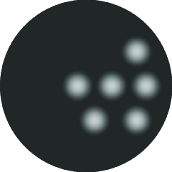
(a) Phantom

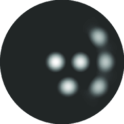
(b) Reconstruction, 5.3 sec.

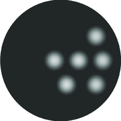
(c) Reconstruction, 10.6 sec.

Figure 1: Reconstructions in the unit disk with model measurement times 5.3 and 10.6 seconds, correspondingly

3.1.1 Numerical example

The following numerical example illustrates how gradual time reversal works in a circular domain. In our simulation the phantom was modeled by a sum of three rotationally symmetric smooth functions defined on the unit disk, as shown in Figure 1(a). The measurements were simulated by tabulating the series solution (equations (43) and (44)) at 1024 equispaced points on the unit circle that represent detectors. Two reconstructions were computed using gradual time reversal with $T=5.3$ sec. and $T=10.6$ sec. of model time. (For comparison, $2$ sec. of model time is the time needed for a wave to propagate once along the diameter of the disk.) These computations were performed using an efficient algorithm [20] for solving the wave equation on a reduced polar grid in a circular domain. The reconstructed images are shown in Figure 1(a) and (b), correspondingly. While the reconstruction with $T=5.3$ sec. is not quite accurate, the image corresponding to $T=10.6$ sec. looks quite close to the original in a gray scale picture. Simulations with larger $T$ (not shown here) yield images that are very close to the phantom not only visually but quantitatively as well.

3.2 Rectangular cavity

A rectangular resonant cavity arises naturally when the object is surrounded by flat detector assemblies that act as reflectors (see, for example, [23]). A very fast Fourier-based reconstruction algorithm has been developed by the authors jointly with B.T. Cox for such a configuration. However, gradual time reversal using finite differences on a Cartesian grid is a much simpler (although slower) method, and, unlike the former algorithm, it can be easily implemented for a variable (but known) speed of sound. In addition, the simplicity of a rectangular domain allows us to illustrate several interesting properties of gradual time reversal.

For simplicity, we present below the 2D case; extension to the 3D is straightforward.

3.2.1 Time reversal with full data

Square domain

(a) Phantom

(b) Reconstruction, 100 sec.

(c) Difference image

Figure 2: Reconstruction of a phantom $\frac{2}{\pi}\cos x_{1}\cos 2x_{2}$ in a square, showing incomplete convergence. The difference between the phantom and the reconstruction (shown on a different gray scale) is very close to $\frac{64}{9\pi^{3}}\sin 2x_{1}\sin x_{2}$

First, let’s assume that the domain $\Omega$ is a square $(0,\pi)\times(0,\pi)$ and that the data are measured on the whole boundary, i.e. $\Sigma_{1}=\Sigma.$ It is convenient to number the eigenfunctions using double indices. In particular, the eigenfunctions $\varphi_{n,l}$ and eigenvalues $\lambda_{n,l}$ needed for solving the forward problem are those of the Neumann Laplacian on $\Omega$:

$$\varphi_{n,l}(x)=N_{n,l}\cos nx_{1}\cos lx_{2},\quad\lambda_{n,l}^{2}=n^{2}+l^{2},\quad n,l=0,1,2,3,...,$$ (53)

with normalization constants $N_{n,l}=\frac{2}{\pi}$ if $n,l>0,$ $N_{0,0}=\frac{1}{\pi},$ $N_{0,1}=N_{1,0}=\frac{\sqrt{2}}{\pi}.$ The eigenfunctions $\psi_{k,m}$ and eigenvalues $\nu_{k,m}$ arising in the analysis of time reversal are those of the Dirichlet Laplacian on $\Omega$:

$$\psi_{k,m}(x)=\frac{2}{\pi}\sin kx_{1}\sin mx_{2},\quad\gamma_{k,m}^{2}=k^{2}+m^{2},\quad k,m=0,1,2,3,...$$

We notice that in the cases $(k,m)=(n,l)$ or $(m,k)=(n,l)$ the eigenvalues coincide; corresponding eigenfunctions are orthogonal in the former case but not always in the latter case:

$$\lambda_{k,m} =\lambda_{m,k}=\gamma_{k,m}=\gamma_{m,k},$$

$$(\psi_{k,m},\varphi_{k,m})_{L_{2}} =0,\quad k,m=0,1,2,3,...$$

$$(\psi_{m,k},\varphi_{k,m})_{L_{2}} =0\quad\text{if }k-m\text{ is even,}$$

$$(\psi_{m,k},\varphi_{k,m})_{L_{2}} \neq 0\quad\text{if }k-m\text{ is odd.}$$

In addition, there are some other pairs of coinciding eigenvalues with non-orthogonal eigenfunctions (e.g. $\lambda_{8,1}=\lambda_{7,4}=\gamma_{8,1}=\gamma_{7,4}$). This implies that the result of the gradual time reversal will not converge to $f(x)$. The residual error will be given by an expression with infinite number of terms similar to (42) (with modifications needed to account for the double indexing of eigenfunctions).

For a simple example, consider initial conditions $f(x)=\varphi_{1,2}(x)=\frac{2}{\pi}\cos x_{1}\cos 2x_{2}.$ Then all coefficients $u_{n,l}$ (except $u_{1,2}=1$) are equal to 0. This implies that gradual time reversal will converge to $f(x)+\mathrm{Err}(x)$ with

$$\mathrm{Err}(x)=-(\psi_{2,1},\varphi_{1,2})_{L_{2}}\psi_{2,1}(x)=\frac{32}{9\pi^{2}}\psi_{2,1}(x)=\frac{64}{9\pi^{3}}\sin 2x_{1}\sin x_{2}.$$ (54)

Figure 2 presents the results of numerical simulation we ran to further illustrate this situation. The model time in this example was about $314$ sec. which corresponds to a hundred bounces of a wave between the opposite sides of a square.  The phantom $f(x)$ is shown in part (a) of the figure, and part (b) shows the reconstruction. Figure 2(c) presents the error in the reconstruction (shown on a different gray scale); it turns out to be very close to the theoretical prediction $\mathrm{Err}(x)$ given by equation (54).

Rectangle with incommensurable sides

Let us now consider a rectangular domain $(0,A)\times(0,B).$ Let us assume that $A$ and $B$ are incommensurable numbers, for example $A$ is rational and $B$ is irrational. Now

$$\varphi_{n,l}(x) =N_{n,l}\cos\frac{\pi nx_{1}}{A}\cos\frac{\pi nx_{2}}{B},\quad\lambda_{n,l}^{2}=\frac{\pi^{2}n^{2}}{A^{2}}+\frac{\pi^{2}l^{2}}{B^{2}},\quad n,l=0,1,2,3,...,$$

$$\psi_{k,m}(x) =\frac{2\pi}{\sqrt{AB}}\sin\frac{\pi kx_{1}}{A}\sin\frac{\pi mx_{2}}{B},\quad\gamma_{k,m}^{2}=\frac{\pi^{2}k^{2}}{A^{2}}+\frac{\pi^{2}m^{2}}{B^{2}},\quad k,m=0,1,2,3,...,$$

where $N_{n,l}=\sqrt{(\varphi_{n,l},\varphi_{n,l})_{L_{2}}}$ are the normalization constants. The only situations when values of $\lambda_{n,l}$ and $\gamma_{k,m}$ coincide is when $(k,m)=(n,l).$ However, it is easy to check by direct computation that in this case $(\psi_{n,l},\varphi_{n,l})_{L_{2}}=0$ and the error terms in the form (42) vanish. Therefore, according to the analysis of Section 2.2, the result of the gradual time reversal will converge weakly (in $H^{1}(\Omega))$ to $f(x)$ as $T\rightarrow\infty.$

3.2.2 Time reversal with partial data

(a) Phantom

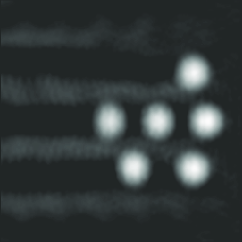
(b) Reconstruction, 100 sec.

(c) Difference image

Figure 3: Reconstruction in a square (a) phantom (b) reconstruction from the data measured on the right side, $T=490$ sec. (c) error shown on a shifted gray scale

We return to the case of the square domain $\Omega=$ $(0,\pi)\times(0,\pi)$,  but this time assume that the measurements are made on only one side of the square, corresponding to $x_{1}=\pi$ (this side plays the role of $\ \Sigma_{1}).$ In this case the eigenfunctions $\varphi_{n,l}(x)$ needed to solve the forward problem are still given by equation (53). To analyze gradual time reversal one needs the eigenfunctions $\psi_{k,m}(x)$ of the Laplacian satisfying Dirichlet boundary condition on the right side of the square and Neumann conditions on the three other sides:

$$\psi_{k,m}(x)=\frac{2}{\pi}\cos\left(\left(k+\frac{1}{2}\right)x_{1}\right)\cos mx_{2},\quad\gamma_{k,m}^{2}=\left(k+\frac{1}{2}\right)^{2}+m^{2},\quad k,m=0,1,2,3,...$$

It follows immediately that, since $\lambda_{n,l}^{2}=n^{2}+l^{2}$ is an integer number and $\gamma_{k,m}^{2}$ is not, $\lambda_{n,l}$ and $\gamma_{k,m}$ never coincide, and therefore the result of gradual time reversal converges weakly in $H^{1}(\Omega)$ to the sought initial condition $f(x)$ as $T\rightarrow\infty.$ It may seem counter-intuitive that time reversal with partial data yields weak convergence while time reversal with full data does not converge. However, this just means that the latter application of this technique is flawed and does not extract full information from the data.

A further look at the eigenfunctions $\psi_{k,m}(x)$ and $\varphi_{n,l}(x)$ reveals that they are orthogonal if $m\neq l,$and, therefore, series representing the error in gradual time reversal will partially decouple similarly to those arising in the analysis of the circular domain.  In general, the rate of convergence of individual modes depends on the differences of eigenvalues (see, for example equations (40) and (41)). If some of these differences are small than the corresponding constant $C_{4}(M,k)$ is large and the convergence will be slow. In the case of the square domain, due to partial orthogonality of eigenmodes, we only need to consider the following differences

$$|\lambda_{n,m}-\gamma_{k,m}|=\left|\sqrt{n^{2}+m^{2}}-\sqrt{\left(k+\frac{1}{2}\right)^{2}+m^{2}}\right|.$$

For large values of $m$ and for $x$ of order of 1 the following Taylor expansion holds

$$\sqrt{m^{2}+x}=m\sqrt{1+x/m^{2}}\thickapprox m+\frac{x}{2m}.$$

Therefore, if $n$ and $k$ are of order of 1 and $m$ is large

$$|\lambda_{n,m}-\gamma_{k,m}|\thickapprox\frac{n^{2}-\left(k+\frac{1}{2}\right)^{2}}{2m};$$

if we let $m$ grow to $\infty$ with fixed $n$ and $k$, the quantity $|\lambda_{n,m}-\gamma_{k,m}|$ converges to 0, which means that convergence of the corresponding modes is getting slower. This implies that even for large values of $T$, the error will contain components with large $m$ and small $k$ manifesting themsselves as waves propagating in the near-vertical direction.

The following numerical example illustrates this situation. Figure 3(a) presents the phantom (the same as in the disk simulation), Figure 3(b) shows the reconstruction corresponding to $T=490$ sec. (or to approximately 156 bounces of a wave between the opposite sides of the square). Figure 3(c) demonstrates the reconstruction error on a shifted gray scale. One can see that in spite of a large value of $T$ in the simulation the error remains noticeable; it consists mostly of the waves with vertical wavefronts as predicted by the above analysis.

This suggests that, if the data is measured on two perpendicular sides of the square, one could use the following reconstruction algorithm: run gradual time reversal separately for each side, filter the two so-obtained images to remove the waves propagating parallel to the acquisition sides, and then add resulting images together. This, indeed, can be done; however, since a fast and rigorously proven method [23] is available for such an acquisition scheme, we will not elaborate further on this topic.

Appendix

In the case of a unit disk domain the eigenvalues $\nu_{m,k}$ and $\lambda_{m,k}$ of the Dirichlet and Neumann Laplacians coincide, correspondingly,  with the positive roots $j_{m,k}$ and $j_{m,k}^{\prime}$ of the Bessel functions $J_{m}(x)$ and its derivative $J_{m}^{\prime}(x)$ (with the exception that $x=0$ is counted as the first zero of $J_{0}^{\prime}(x)$ and not counted for $J_{m}^{\prime}(x)$ with $m>0)$. In this section we establish the fact that the distance between these roots is uniformly bounded from below (in the sense of equation (49)).

It is well known that the roots of $J_{m}(x)$ and $J_{m}^{\prime}(x)$ interlace [43, 1]:

$$j_{m,k}<j_{m,k+1}^{\prime}<j_{m,k+1},\qquad k=1,2,3,...$$

It is also known that for $m>0$ all non-zero roots are greater than $m$; more precisely [43]:

$$j_{m,1}>j_{m,1}^{\prime}>\sqrt{m(m+2)},\qquad m>0,$$

and that asymptotically (for large $k$ and fixed $m)$ these roots become equispaced [1]:

$$j_{m,k} \sim\left(k+\frac{1}{2}m-\frac{1}{4}\right)\pi,$$ (55)

$$j_{m,k}^{\prime} \sim\left(k+\frac{1}{2}m-\frac{3}{4}\right)\pi.$$ (56)

Therefore, as $k\rightarrow\infty$

$$j_{m,k}-j_{m,k}^{\prime} \rightarrow\frac{\pi}{2},$$

$$j_{m,k+1}^{\prime}-j_{m,k} \rightarrow\frac{\pi}{2}.$$

We, however, need a uniform lower bound on $|j_{m,k}-j_{m,l}^{\prime}|$ valid for all values of $m,$ $k,$ and $l.$ Such a bound on the distance between the roots of $J_{m}(x)$ is known [14]:

$$|j_{m,k}-j_{m,l}|>\pi|k-l|,\qquad m>1/2.$$ (57)

In addition, we need the following result which we have not found in the literature:

Lemma 3

For any $m\geq 1$ ($m$ does not have to be integer) the distance between the adjacent roots of $J_{m}^{\prime}$ and $J_{m}$ is uniformly bounded:

$$j_{m,k}-j_{m,k}^{\prime} \geq\sqrt{2},\qquad k=2,3,4,...$$ (58)

$$j_{m,k+1}^{\prime}-j_{m,k} \geq 1,\qquad k=1,2,3,...$$ (59)

Proof. Let us consider the open interval $I_{k}=(j_{m,k},j_{m,k+1})$ between the adjacent zeros of $J_{m}.$ Let us first assume that $J_{m}$ is positive on $I_{k}.$ Then $J_{m}$ attains its local maximum $\max\limits_{I_{k}}J_{m}(x)$ at the point $j_{m,k+1}^{\prime}\in I_{k}.$ Recall that $J_{m}$ satisfies the Bessel equation

$$x^{2}J_{m}^{\prime\prime}(x)+xJ_{m}^{\prime}(x)+(x^{2}-m^{2})J_{m}(x)=0,$$

which for $x>0$ can be re-written in the following form:

$$\left(xJ_{m}^{\prime}(x)\right)^{\prime}=-\frac{x^{2}-m^{2}}{x}J_{m}(x).$$ (60)

By integrating the latter equation from $j_{m,k+1}^{\prime}$ to $x$ we obtain

$$J_{m}^{\prime}(x)=-\frac{1}{x}\int\limits_{j_{m,k+1}^{\prime}}^{x}\frac{t^{2}-m^{2}}{t}J_{m}(t)dt.$$ (61)

Now let us use equation (61) and integrate $-J_{m}^{\prime}(x)$ from $j_{m,k+1}^{\prime}$ to $j_{m,k+1},$ taking into account that $J_{m}(j_{m,k+1})=0,$ that $\max_{I_{k}}J_{m}(x)=J_{m}(j_{m,k+1}^{\prime}),$ and that $t>m$ on $(j_{m,k+1}^{\prime},j_{m,k+1})$:

$$\max_{I_{k}}J_{m}(x)=\int\limits_{j_{m,k+1}^{\prime}}^{j_{m,k+1}}\frac{1}{x}\left[\int\limits_{j_{m,k+1}^{\prime}}^{x}\frac{t^{2}-m^{2}}{t}J_{m}(t)dt\right]dx\leq\max_{I_{k}}J_{m}(x)\int\limits_{j_{m,k+1}^{\prime}}^{j_{m,k+1}}\frac{1}{x}\left[\int\limits_{j_{m,k+1}^{\prime}}^{x}tdt\right]dx.$$

Dividing both sides of the above inequality by $\max\limits_{I_{k}}J_{m}(x)$ yields:

$$1 \leq\int\limits_{j_{m,k+1}^{\prime}}^{j_{m,k+1}}\frac{1}{x}\left[\int\limits_{j_{m,k+1}^{\prime}}^{x}tdt\right]dx=\int\limits_{j_{m,k+1}^{\prime}}^{j_{m,k+1}}\frac{1}{2x}(x-j_{m,k+1}^{\prime})(x+j_{m,k+1}^{\prime})dx$$

$$\leq\int\limits_{j_{m,k+1}^{\prime}}^{j_{m,k+1}}(x-j_{m,k+1}^{\prime})dx=\frac{(j_{m,k+1}-j_{m,k+1}^{\prime})^{2}}{2}.$$

Therefore

$$j_{m,k+1}-j_{m,k+1}^{\prime}\geq\sqrt{2}.$$

Similarly, in order to bound $j_{m,k+1}^{\prime}-j_{m,k},$ integrate equation (61) from $j_{m,k}$ to $j_{m,k+1}^{\prime}$:

$$\max_{I_{k}}J_{m}(x)=\int\limits_{j_{m,k}}^{j_{m,k+1}^{\prime}}\frac{1}{x}\left[\int\limits_{x}^{j_{m,k+1}^{\prime}}\frac{t^{2}-m^{2}}{t}J_{m}(t)dt\right]dx\leq\max_{I_{k}}J_{m}(x)\int\limits_{j_{m,k}}^{j_{m,k+1}^{\prime}}\frac{1}{x}\left[\int\limits_{x}^{j_{m,k+1}^{\prime}}\frac{t^{2}-m^{2}}{t}dt\right]dx.$$

By dividing both sides by $\max\limits_{I_{k}}J_{m}(x)$ we obtain:

$$1 \leq\int\limits_{j_{m,k}}^{j_{m,k+1}^{\prime}}\frac{1}{x}\left[\int\limits_{x}^{j_{m,k+1}^{\prime}}\frac{t^{2}-m^{2}}{t}dt\right]dx\leq\int\limits_{j_{m,k}}^{j_{m,k+1}^{\prime}}\frac{2}{x}\left[\int\limits_{x}^{j_{m,k+1}^{\prime}}(t-m)dt\right]dx$$

$$\leq\int\limits_{j_{m,k}}^{j_{m,k+1}^{\prime}}\frac{1}{x}\left[j_{m,k+1}^{\prime}-x^{2}-2m(j_{m,k+1}^{\prime}-x)\right]dx\leq\int\limits_{j_{m,k}}^{j_{m,k+1}^{\prime}}(j_{m,k+1}^{\prime}-x)\frac{j_{m,k+1}^{\prime}+x-2m}{j_{m,k}}dx$$

$$\leq\frac{2(j_{m,k+1}^{\prime}-m)}{j_{m,k}}\int\limits_{j_{m,k}}^{j_{m,k+1}^{\prime}}(j_{m,k+1}^{\prime}-x)dx=(j_{m,k+1}^{\prime}-j_{m,k})^{2}\frac{j_{m,k+1}^{\prime}-m}{j_{m,k}}$$

$$\leq(j_{m,k+1}^{\prime}-j_{m,k})^{2}\frac{j_{m,k+1}^{\prime}-1}{j_{m,k}},$$

which implies $j_{m,k+1}^{\prime}-j_{m,k}\geq 1.$ This proves the Lemma for all intervals $I_{k}$ on which $J_{m}$ is positive. In order to prove it for the intervals where $J_{m}$ is negative, replace $J_{m}$ by $-J_{m}$ and repeat the proof above.   

Proposition 2

There is constant $C>0$ such that for any integer numbers $m\geq 0,$ $k\geq 1,$ and $l\geq 1$ the distance between the roots $j_{m,l}$ of $J_{m}$ and $j_{m,k}^{\prime}$ of $J_{m}^{\prime}$ is bounded from below:

$$\left|j_{m,k}-j_{m,l}^{\prime}\right|\geq C\left|2k-2l+1\right|$$ (62)

Proof. First consider any function $J_{m}$ for $m\geq 1.$ If $l\leq k,$ due to (58) and (57),

$$j_{m,k}-j_{m,l}^{\prime}\geq\sqrt{2}+\pi(k-l)$$

and (62) holds if one chooses $C=1$ (this is clearly not the sharpest bound!). In the case when $l>k,$ using (59) and (57) we obtain

$$j_{m,l}^{\prime}-j_{m,k}\geq 1+\pi(l-k-1),$$

and (62) again holds if one chooses $C=1.$ This proves (62) for all roots of functions $J_{m}$ with $m\geq 1$. Now, let us consider the function $J_{0}(x).$ Due to the asymptotic behavior of the roots (see equations (55) and (56)), there are constants $C_{0}$ and $C_{1}$ such that

$$\left|j_{0,k}-j_{m,n}\right| \geq C_{0},\qquad k,n=1,2,3,...$$

$$j_{0,k}-j_{0,k}^{\prime} \geq C_{1},\qquad k=1,2,3,...$$

$$j_{0,k+1}^{\prime}-j_{0,k} \geq C_{1},\qquad k=1,2,3,...$$

with $C_{1}\leq C_{0}/2.$ Then the following inequality holds:

$$\left|j_{0,k}-j_{0,l}^{\prime}\right|\geq C_{1}\left|2k-2l+1\right|,\qquad k,l=1,2,3,...$$

Set $C=\operatorname{min}(1,C_{1})$ and (62) holds for all values of $m,l,k$ of interest.

References

• [1] Abramowitz M and Stegun I A 1964 Handbook of Mathematical Functions With Formulas, Graphs, and Mathematical Tables National Bureau of Standards, Washington, D.C.
• [2] Ambartsoumian G and Kuchment P 2005 On the injectivity of the circular Radon transform. Inverse Problems 21 473–85
• [3] Agranovsky M and Kuchment P 2007, Uniqueness of reconstruction and an inversion procedure for thermoacoustic and photoacoustic tomography with variable sound speed Inverse Problems 23 2089–102
• [4] Agranovsky M, Kuchment P, and Quinto E T 2007 Range descriptions for the spherical mean Radon transform J. Funct. Anal. 248 344–86
• [5] Agranovsky M and Quinto E T 1996 Injectivity sets for the Radon transform over circles and complete systems of radial functions. J. Funct. Anal. 139 383–414
• [6] Agranovsky M and Nguyen L V 2010 Range conditions for a spherical mean transform and global extendibility of solutions of the Darboux equation Journal D Analyse Mathematique 112 351–67
• [7] Agranovsky M, Finch D and Kuchment P 2009 Range conditions for a spherical mean transform Inverse Problems And Imaging 3(3) 373–82
• [8] Ammari H, Bossy E, Jugnon V and Kang H 2010 Mathematical modeling in photoacoustic imaging of small absorbers SIAM Review 52(4) 677–95
• [9] Beard P C 2011 Biomedical Photoacoustic Imaging Interface Focus 1(4) 602–31
• [10] Burgholzer P, Matt G J, Haltmeier M, and. Paltauf G 2007 Exact and approximative imaging methods for photoacoustic tomography using an arbitrary detection surface Phys Review E 75 046706
• [11] Cox B T, Arridge S R and Beard P C 2007 Photoacoustic tomography with a limited-aperture planar sensor and a reverberant cavity Inverse Problems 23(6) S95–S112
• [12] Cox B T and Beard P C 2009 Photoacoustic tomography with a single detector in a reverberant cavity J. Acoust. Soc. Am. 125(3) 1426–36
• [13] Cox B T, Laufer J, Arridge S R et al 2012 Quantitative spectroscopic photoacoustic imaging: a review J. Of Biomedical Optics 17(6) 061202
• [14] Elbert A and Laforgia A 1986 Monotonicity properties of the zeros of Bessel functions SIAM J. Math. Anal. 17(6) 1483–88
• [15] Ellwood R, Zhang E Z, Beard P C and Cox B T 2014 Photoacoustic imaging using acoustic reflectors to enhance planar arrays, submitted
• [16] Finch D, Haltmeier M and Rakesh 2007 Inversion of spherical means and the wave equation in even dimensions SIAM J. Appl. Math. 68(2) 392–412
• [17] Finch D, Patch S K, and Rakesh 2004 Determining a function from its mean values over a family of spheres SIAM J. Math. Anal. 35(5) 1213–40
• [18] Fleckinger-Pelle J 1985 Asymptotics of eigenvalues for some “non-definite” elliptic problems volume 1151 of Lecture Notes in Mathematics 148–156 Springer-Verlag, Berlin
• [19] Hristova Y, Kuchment P and Nguyen L 2008 On reconstruction and time reversal in thermoacoustic tomography in homogeneous and non-homogeneous acoustic media Inverse Problems 24 055006
• [20] Holman B 2014 A second-order finite difference scheme for the wave equation on a reduced polar grid. Preprint
• [21] Kruger R A, Liu P, Fang Y R and Appledorn C R 1995 Photoacoustic ultrasound (PAUS) reconstruction tomography Med. Phys. 22 1605–09
• [22] Kruger R A, Reinecke D R, and Kruger G A 1999 Thermoacoustic computed tomography - technical considerations Med. Phys. 26 1832–7
• [23] Kunyansky L, Holman B and Cox B T 2013 Photoacoustic tomography in a rectangular reflecting cavity Inverse Problems 29 125010
• [24] Kunyansky L 2007 Explicit inversion formulae for the spherical mean Radon transform Inverse problems 23 737–83
• [25] Kunyansky L 2007 A series solution and a fast algorithm for the inversion of the spherical mean Radon transform Inverse Problems, 23 (2007) S11–S20
• [26] Kunyansky L 2011 Reconstruction of a function from its spherical (circular) means with the centers lying on the surface of certain polygons and polyhedra Inverse Problems 27 025012
• [27] Ladyzhenskaya O A 1985 The Boundary Value Problems of Mathematical Physics, volume 49 of Applied Mathematical Sciences Springer-Verlag, New York
• [28] Natterer F 2012 Photo-acoustic inversion in convex domains Inverse Problems Imaging 6 315—20
• [29] Norton S J 1980 Reconstruction of a two-dimensional reflecting medium over a circular domain: exact solution J. Acoust. Soc. Am. 67 1266–73
• [30] Norton S J and Linzer M 1981 Ultrasonic reflectivity imaging in three dimensions: exact inverse scattering solutions for plane, cylindrical, and spherical apertures IEEE Tran. Biomed. Eng. 28 200–2
• [31] Nguyen L V 2009 A family of inversion formulas in thermoacoustic tomography Inverse Problems and Imaging 3(4) 649–75
• [32] Oraevsky A A, Jacques S L, Esenaliev R O and Tittel F K 1994 Laser-based photoacoustic imaging in biological tissues  Proc. SPIE 2134A 122–8
• [33] Palamodov V P 2012 A uniform reconstruction formula in integral geometry Inverse Problems 28 065014
• [34] Pulkkinen A, Cox B T, Arridge S R et al 2014 A Bayesian approach to spectral quantitative photoacoustic tomography Inverse Problems 30(6) 065012
• [35] Qian J, Stefanov P, Uhlmann G et al 2011 An efficient neumann series-based algorithm for thermoacoustic and photoacoustic tomography with variable sound speed SIAM J. On Imaging Sciences 4(3) 850–83
• [36] Quinto E T and Rullgard H 2013 Local singularity reconstruction from integrals over curves in $\mathbb{R}^{3}$ Inverse Problems and Imaging 7(2) 585–609
• [37] Salman Y 2014 An inversion formula for the spherical mean transform with data on an ellipsoid in two and three dimensions J. Math. Anal. Appl. 420 612—20
• [38] Scherzer O (Editor) (2011) “Handbook of Mathematical Methods in Imaging” (Springer).
• [39] Stefanov P and Uhlmann G 2011 Thermoacoustic tomography arising in brain imaging Inverse Problems 27(4) 045004
• [40] Tarvainen T, Pulkkinen A, Cox B T et al 2013 Bayesian Image Reconstruction in Quantitative Photoacoustic Tomography IEEE Trans. On Med. Imag. 32(12) 2287–98
• [41] Wang L V and Yang X 2007 Boundary conditions in photoacoustic tomography and image reconstruction J. Biomed. Opt. 12(1) 014027
• [42] Wang L V (Editor) 2009 “Photoacoustic imaging and spectroscopy” (CRC Press).
• [43] Watson G N 1966 A Treatise on the Theory of Bessel Functions Cambridge University Press, London, New York, 2-nd edition
• [44] Xu M and Wang L V 2004 Time reversal and its application to tomography with diffracting sources Phys. Rev. Lett. 92(3) 3–6
• [45] Xu M and Wang L V 2005 Universal back-projection algorithm for photoacoustic computed tomography Phys. Rev. E 71 016706.