Validating Velocities in the GeoClaw Tsunami Model using Observations Near Hawaii from the 2011 Tohoku Tsunami

Abstract

The ability to measure, predict, and compute tsunami flow velocities is of importance in risk assessment and hazard mitigation. Substantial damage can be done by high velocity flows, particularly in harbors and bays, even when the wave height is small. Moreover, advancing the study of sediment transport and tsunami deposits depends on the accurate interpretation and modeling of tsunami flow velocities and accelerations. Until recently, few direct measurements of tsunami velocities existed to compare with model results. During the 11 March 2011 Tohoku Tsunami 328 current meters were in place around the Hawaiian Islands, USA, that captured time series of water velocity in 18 locations, in both harbors and deep channels, at a series of depths. We compare several of these velocity records against numerical simulations performed using the GeoClaw numerical tsunami model, based on solving the depth-averaged shallow water equations with adaptive mesh refinement, to confirm that this model can accurately predict velocities at nearshore locations. Model results demonstrate tsunami current velocity is more spatially variable than wave form or height and therefore may be a more sensitive variable for model validation.

1 Introduction

In the last decade, tsunamis have resulted in millions of dollars in damage far from their sources. Often this damage was not the result of high flow depth or long inundation distances, but rather due to the strong currents generated in harbors and along coastlines. In the last ten years, tsunamis have generated over $170 million damage in U.S. states and territories. For example, the Mw 9.0 2011 Tohoku tsunami alone is estimated to have caused $90 million in damages in the U.S., even though the highest waves arrived near low tide and there was little on-shore inundation (The Western States Seismic Policy Council (2011)), and the Mw 8.3 2006 Kuril Island earthquake generated a tsunami that caused $20 million in damage to the Crescent City, California, harbor (Dengler and Uslu (2011)). These costs highlight the need to understand and predict the velocities of currents generated by tsunamis in harbors and channels. A recent study by Lynett et al (2014) illustrates that tsunami current velocities between 3 and 6 knots (roughly 1.5 to 3 m/s) can cause moderate damage while velocities above 6 knots can cause major damage.

The study of sediment transport and tsunami deposits also depends on knowledge of flow velocities and accelerations (Apotsos et al (2011)). Determining potential for sediment transport and the source location of sediment transported is of importance in establishing the frequency and magnitude of past events based on the study of tsunami deposits (Bourgeois (2009); Huntington et al (2007)). Recent studies have focused on tsunami velocities and flow parameters based on interpreting the source of sediment (e.g., Moore et al (2007); Sawai et al (2009)). Accurate modeling of locations and depths of strong flow and accelerations would aid in determining possible sediment source locations. Better understanding of tsunami current velocities may also be important in exploring the depth at which tsunamis erode and deposit sediment, and whether tsunamis can leave submarine records (Weiss (2008)).

Numerical tsunami models are frequently validated using only wave height and inundation data, which is now plentiful from recent events (e.g., Liu et al (2005); Synolakis and Okal (2005); Satake et al (2006); MacInnes et al (2009, 2013); Okal et al (2010); Fritz et al (2011)), Surface elevation from Deep-Ocean Assessment and Reporting of Tsunamis (DART) buoys or other deep-ocean monitors as well as from coastal and harbor tide gauges are used, along with inundation and runup data collected by tsunami survey teams following every major event (e.g., Synolakis et al (2007); Apotsos et al (2011)). See in particular the work of Tang et al (2009), which concerns validation of the MOST tsunami model using data around Hawaii from several past tsunamis.

The ability to measure and compute tsunami velocities remains at the frontier of tsunami science. Tsunami models calculate depth-averaged water velocity, but until recently there have been few data sets available to validate the model results. Recent studies have begun to compare tsunami velocity simulations with laboratory results, post-tsunami survey data and analysis of survivor videos, or direct measurement from current meters. Limited data are available of directly measured tsunami currents. In the nearfield, tsunami flow velocities have been calculated from video analysis of floating objects (up to 11 m/s) (Fritz et al (2006, 2012); Earthquake Engineering Research Institute (2011)), damage to structures (5-8 m/s) (Earthquake Engineering Research Institute (2011)), and sediment transport (up to 14 m/s) Apotsos et al (2011); Jaffe and Gelfenbaum (2007). The Maule, Chile tsunami was observed with velocities up to 0.36 m/s in Monterey Bay, California (Lacy et al (2012)). Current meter data in the farfield were also recorded during the 2011 Tohoku event in Humboldt Bay (0.36 – 0.84 m/s; Admire (2013); Admire et al (2014)) and in New Zealand (Lynett et al (2012)). Some currents were observed in Hawaii during the 2006 Kuril Island event (Bricker et al (2007)). Other studies have used video or ship GPS analysis in farfield harbors (e.g., Admire (2013); Admire et al (2014); Lynett et al (2012)).

Tsunami modeling assumptions and validation can be tested with these data. For example, Apotsos et al (2011) compared numerical simulations to both laboratory experiments and field estimates of velocities during the 2004 Sumatra event. In Jaffe and Gelfenbaum (2007); Fritz et al (2006, 2012); Earthquake Engineering Research Institute (2011), tsunami current speeds interpreted from different tsunami events vary between 5 m/s and 14 m/s in the near field. Direct measurements of tsunami velocity (up to 0.14 m/s) were obtained by current meters deployed to monitor coral reef environments that serendipitously measured the 2006 Kuril Island tsunami (Bricker et al (2007)) at 40 depths in a water depth of 10 m off the coast of Honolulu, Hawaii. These were used to test the assumptions of shallow water wave equations with real world observations (Arcas and Wei (2011)). Lacy et al (2012) observed the currents of the 2010 Maule, Chile tsunami at three depths in Monterey Bay, California, recording velocities up to 0.36 m/s. Higher velocities have been measured by analyzing survivor videos of tsunami inundation near to the tsunami source. Velocities of up to 5 m/s and 11 m/s were measured of the 2004 tsunami on the coast of Banda Aceh, Indonesia and the 2011 Tohoku tsunami on the Sanriku coast of Japan respectively (Fritz et al (2006, 2012)). In the Tohoku region of Japan, video analysis esimated a flow velocity of 6.89 m/s during the 2011 tsunami (Earthquake Engineering Research Institute (2011)). Based on flow depth and analysis of the properties of building materials damaged in the 2011 tsunami on the Sendai Plain, flow velocity estimates ranging from 5-8 m/s (Earthquake Engineering Research Institute (2011)) were obtained. Using modeling of sedimentary data of the 1998 Papua New Guinea tsunami a velocity of 14 m/s was interpreted by Jaffe and Gelfenbaum (2007). Admire (2013) and Admire et al (2014) studied currents induced by the Tohoku event in Crescent City Harbor (estimated from video, up to 4.5 m/s) and Humboldt Bay (measured by a current meter with a peak amplitude of 0.84 m/s), and compared with numerical simulations. Lynett et al (2012) studied currents and vortical structures in several ports and harbors induced by the Tohoku event.

It is important to note that velocities often exhibit much greater spatial variability than flow depth, particularly in bays and harbors, and we present several figures to illustrate this. This may seem counter-intuitive for a model based on the shallow water equations since for a long-wavelength coherent tsunami wave (e.g. in the ocean away from shorelines) there is a direct relationship between the surface elevation and the depth-averaged velocity, with $s\approx\eta/\sqrt{h_{0}}$ where $s$ is the speed, $\eta$ the surface displacement, and $h_{0}$ the undisturbed depth. But this is only true for a plane wave moving in one direction on a flat bottom. Anywhere there is a superposition of waves moving in different direction (via reflections from shorelines and/or bathymetric features) there is no longer such a clean relationship. In shallow water near shore, the relationship will be even less clean because of the interaction with bathymetry over short spatial scales on a much more finely resolved grid, and the generation of vorticity and complex flows in harbors further complicate the picture. This increases both the importance and difficulty of validating tsunami models against observed velocities.

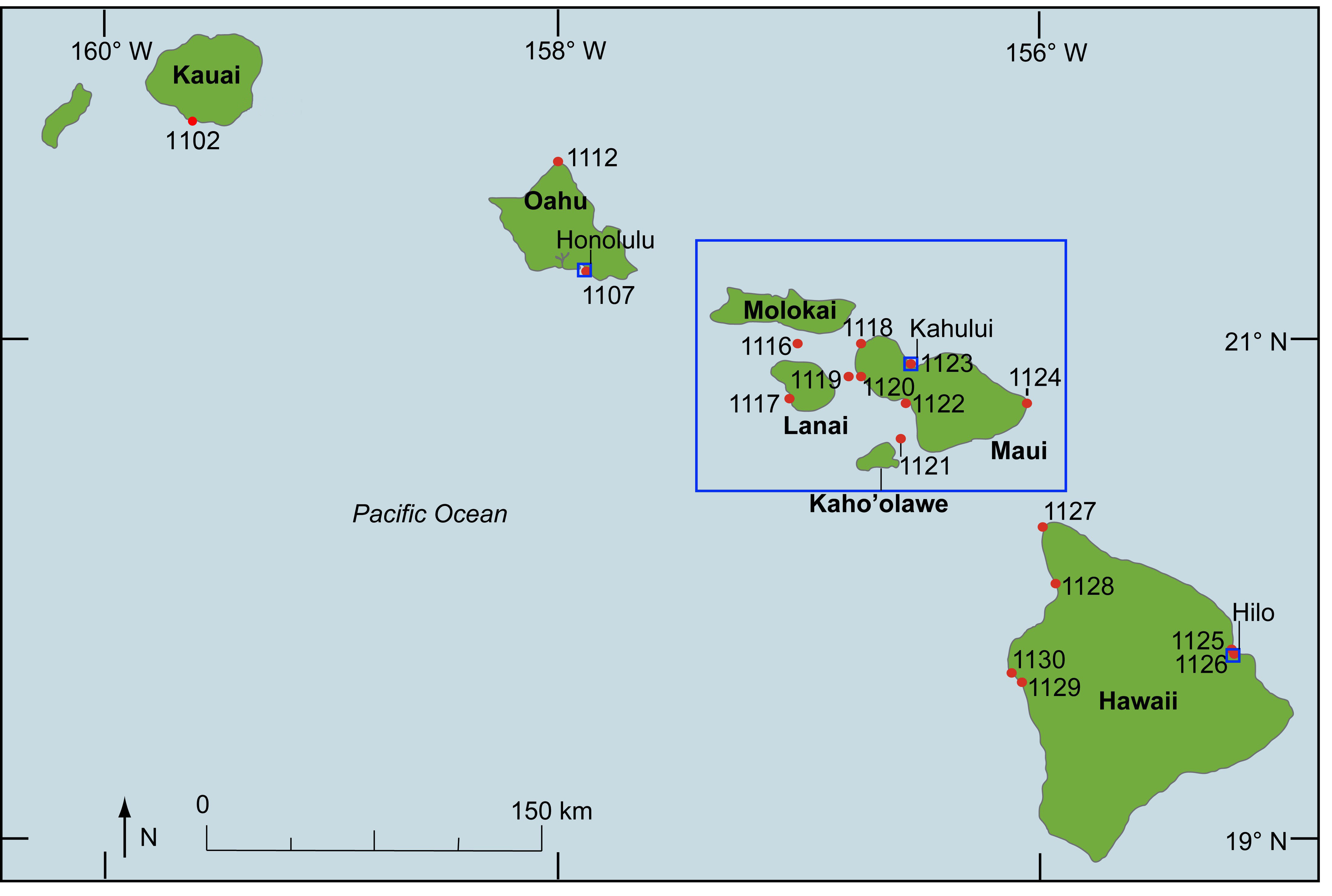
Figure 1: Map showing the location of current velocity meter stations deployed around Hawaii, including the ten stations used in this study. Blue boxes denote the location of later maps.

In this study, we explore the use of a data set from Hawaii for the purpose of validating a numerical model. During the 11 March 2011 Tohoku Tsunami, there were 328 current meters in place around the islands of Hawaii that captured time series of the fluid velocity at varying depths of water within the water column at 18 different locations (stations) (Co-Ops Survey (Accessed 23 September 2011)) as shown in Figure 1. Not only are these data direct measurements of the 2011 tsunami but they cover a much wider range of bathymetric conditions than many previous studies including open coastline, deep channels and harbors. We have compared ten stations with simulations performed using the GeoClaw software described in Section 2, which solves the depth-averaged shallow water equations. Section 3 describes observations and simulation results. These validation results are presented in Section 4. At most of these stations the numerical model reproduces depth-averaged versions of the measured data quite well, although the agreement is not as good at the stations that are inside harbors, as discussed further in Sections 4 and 6.

The past studies that are most aligned with this paper are the work of Cheung et al (2013), who also performed velocity comparisons for all the stations used in this paper, and Yamazaki et al (2012), where velocity comparisons are made at the Kilo Nalu Observatory near Honolulu Harbor. In both case the numerical simulations were performed using the NEOWAVE code. The Kilo Nalu Observatory is indicated as KN in Figure 6, and discussed further in Section 4.

2 The GeoClaw numerical model

The open source GeoClaw tsunami model (GeoClaw authors (2012)) was used to perform numerical simulations. This model has undergone extensive validation and verification tests as reported in LeVeque and George (2007); Berger et al (2011); González et al (2011); LeVeque et al (2011), using both synthetic test problems and real events, but always based on comparing surface elevations or inundation. This paper presents the first comparisons of GeoClaw results with current data and, as far as we know, the first direct, quantitative comparison of observed time series data from velocity meters to modeled results over such a broad area and variety of settings.

The GeoClaw software implements high-resolution finite volume methods to solve the nonlinear shallow water equations, a depth-averaged system of partial differential equations in which the fluid depth $h(x,y,t)$ and two horizontal depth-averaged velocities $u(x,y,t)$ and $v(x,y,t)$ are introduced. $u$ is defined as the eastward and $v$ is defined as the northward velocity component. These equations are written in a form that corresponds to conservation of mass and momentum whenever the terms on the right hand side vanish:

$$\begin{split}h_{t}+(hu)_{x}+(hv)_{y}&=0,\\ (hu)_{t}+\left(hu^{2}+\frac{1}{2}gh^{2}\right)_{x}+(huv)_{y}&=-ghB_{x}-Dhu,\\ (hv)_{t}+(huv)_{x}+\left(hv^{2}+\frac{1}{2}gh^{2}\right)_{y}&=-ghB_{y}-Dhv,\end{split}$$ (1)

Subscripts denote partial derivatives. The momentum source terms on the right hand side involve the varying bathymetry $B(x,y,t)$ and a frictional drag term, where $D(h,u,v)$ is a drag coefficient given by

$$D(h,u,v)=n^{2}gh^{-4/3}\sqrt{u^{2}+v^{2}}.$$ (2)

The parameter $n$ is the Manning coefficient and depends on the roughness. If detailed information about the seafloor or inundated region is known, then this could be a spatially varying parameter. For generic tsunami modeling a constant value of $n=0.025$ is often used. The value $n=0.035$ has been suggested to better account for the fringing reefs surrounding the Hawaiian Islands by Bretschneider et al (1986), and in this study we used this latter value, but also ran all of our simulations with the smaller value and found virtually identical results. This is to be expected since the friction term generally makes a difference only in very shallow water. The choice of Manning coefficient can make a significant difference for inundation studies, but not for the off-shore flow studied here.

Coriolis terms can also be added to the right hand side of equations (1), but these generally have been found to be negligible in tsunami modeling (e.g., Dao and Tkalich (2007); Kirby et al (2013)). We have performed all of our computations both with and without the Coriolis terms and have confirmed this for the case studied here — there is no visible difference in the gauge results when Coriolis terms are added.

Other than the Manning friction coefficient, there are no tunable parameters in the GeoClaw model. The sea level parameter in the code can also be varied to adjust the initial water level. We have used the vertical datum of the bathymetry data, which for the nearshore bathymetry is referenced to Mean High Water (MHW). For modeling inundation, it may be important to more carefully set the tide stage and Manning coefficient, but for the offshore gauges the differences are negligible.

The finite volume methods implemented in GeoClaw are based on dividing the computational domain into rectangular grid cells and storing cell averages of mass and momentum in each grid cell. These are updated each time step by a high-resolution Godunov type method (LeVeque (2002)) that is based on solving Riemann problems at the interfaces between neighboring grid cells and applying nonlinear limiters to avoid nonphysical oscillations. These methods are second order accurate in space and time wherever the solution is smooth, but robustly handle strong shock waves and other discontinuous solutions. This is important when the tsunami reaches shallow water and hydraulic jumps arise from wave breaking. Also, the methods have been extended to deal robustly with inundation. Grid cells where $h=0$ represent dry land and cells can dynamically change between wet and dry each time step.

Block structured adaptive mesh refinement is used to employ much finer grid resolution in regions of particular interest. Regions of refinement track the tsunami as it propagates across the ocean, and then additional levels of refinement are added around Hawaii and even finer grids in the regions around the gauges of interest. For the calculations presented here, a grid resolution of $2^{\circ}$ was used at the coarsest level, Five additional nested levels of refinement were generally used, generally going down to $1^{\prime\prime}$ resolution on the finest grid for gauges away from harbors (1 arcsecond is about 30 meters). For simulations of Hilo and Kahului Harbors the finest level was reduced to $1/3^{\prime\prime}$, while for the larger region surrounding Honolulu Harbor the finest level was $2/3^{\prime\prime}$. Runs at finer resolution were used to confirm that the results shown here are well resolved.

In addition to refining the spatial resolution, smaller timesteps must be used on the finer grid patches. The GeoClaw software implements the timestepping and transfer of information between grids at different levels, as well as the automatic flagging of grid cells requiring refinement and the clustering of these cells into rectangular patches for refinement to the next level. More details of these numerical methods can be found in George (2006); George and LeVeque (2006); George (2008); LeVeque et al (2011). Version 5.2.1 of the GeoClaw code was used to produce the final figures in this publication.

The ETOPO1 global bathymetry (Amante and Eakins (2009)) was used over the ocean, at 1 minute resolution. Around the Hawaiian Islands bathymetry from the National Geophysical Data Center was used, with resolution of $6^{\prime\prime}$, together with finer $1/3^{\prime\prime}$ grids around Hilo and Honolulu Harbors (National Geophysical Data Center (Accessed 17 February 2012)). Near Kahului Harbor $1^{\prime\prime}$ resolution is the finest available and this was used, and interpolated to $1/3^{\prime\prime}$ by the GeoClaw code. GeoClaw combines data from different data sets into a global piecewise bilinear function that can be integrated over each computational grid cell in order to obtain the cell average of the bathymetry. This is done in a manner that is consistent between different grid levels in order to maintain conservation of mass.

The initial seafloor deformation for the tsunami simulations was based on Fujii et al (2011), which was calculated using tsunami waveform inversion based on DART buoy, tidegauge and GPS gauge data. This seafloor deformation was previously found to be one of the best at replicating nearfield run-up and DART buoy time series in a recent comparison of GeoClaw results using ten proposed sources for the Tohoku event in the study of MacInnes et al (2013).

3 Tsunami observations

In order to evaluate shipping lanes and harbors, the National Oceanic and Atmospheric Administration deployed 30 current meter stations with horizontal 2-D Acoustic Doppler Profilers (Sontek/YSIH - ADP) off the Hawaiian Islands in early 2011 as part of the 2011 Hawaii Current Observation Project (Co-Ops Survey (Accessed 23 September 2011)). Eighteen stations were active and recorded the passing of the Tohoku tsunami. The station locations are tabulated with additional information in Table 1 and are shown in Figure 1, and in more detail near the harbors in Figures 6 through 12.

Water depth at the active stations varied between 12.5 and 153 m. Current meters were approximately evenly spaced at varying depths along a cable, with 6 to 34 current meters at each station with an increasing number of current meters with increasing depth. The deepest current meters were between 1.6 and 29 m from the seafloor and the shallowest were 2 to 17 m below the sea surface. The current meters record speed and horizontal direction at six-minute time intervals. The six-minute sample interval captures variation in velocity with the inflow and outflow of long period tsunami waves but may not capture other types of waves such as edge waves (periods of three or more minutes) that are excited by the tsunami and have been observed with more detailed sample intervals (Bricker et al (2007); Cheung et al (2013)). Accuracy of the current meters is $\pm 0.5$ cm/s speed and $\pm 2$ degrees for direction. Wave amplitude and vertical motion were not recorded (Co-Ops Survey (Accessed 23 September 2011)). Vertical flow in offshore tsunami waves is generally negligible compared to horizontal flow (Arcas and Wei (2011)).

In this paper we present results for ten of these stations that test the ability of our numerical model to reproduce the primary characteristics of tsunami currents in different settings. We focus on stations that are in protected water, primarily in the channels between the islands of Maui, Molokai, and Lanai and near the harbors of Honolulu, Kahului, and Hilo. At these stations there is a strong tsunami signal visible in the record for many hours after the arrival of the first wave, typically because of seiching in these protected regions. These are also the regions where tsunami currents are of most interest in relation to hazards to harbors and shipping. The stations studied include four in quite shallow water, less than 25 m depth, near the harbors and bays (HAI1107, HAI1123, HAI1125, and HAI1126), and six others in in the inter-island channels (HAI1116, HAI1118, HAI1119, HAI1120, HAI1121, HAI1122). With the exception of HAI1120 (near Lahaina), these are in 25–150 m depth.

From the speed and direction of flow that was recorded at each depth, we computed the east-west velocity $u$ and north-south velocity $v$. Two samples of these records are shown in Figure 2, for a 48-hour window around the tsunami arrival time. The top of Figure 2 shows HAI1107, in the approach to Honolulu Harbor. In this shallow location (14.9 m) there is very little variation in velocity with depth. Figure 2 also shows HAI1119, at 73.51 m depth in the Auau Channel, where the greatest variation of velocity with depth was observed.

Like all other codes for modeling transoceanic tsunamis, the GeoClaw software computes a single depth-averaged velocity at each point and cannot directly model the velocity profile with depth. For comparison purposes, we depth-averaged the observed $u$ and $v$ velocities at each depth to obtain a single velocity time series at each station. This depth-averaged velocity is also shown in the right panel of Figure 2. Note that the current meters generally did not span the entire water column from seafloor to surface. Hence we are averaging over only a subset of the water column. Since the shallow water equations assume a constant velocity with depth, we believe this gives the best value for comparison with the numerical results.

Current meter data has been filtered to remove tidal currents. Because the data appears so noisy, even before the arrival of the tsunami, we explored two different approaches to detiding the data and found that they gave nearly identical results, increasing our confidence in the results. In both cases a least squares fit to a 48-hour time series of data starting 20 hours before the earthquake was computed. One approach was to fit a high degree polynomial, and we found that a degree 20 polynomial was able to match the tidal oscillations in this length data without introducing higher frequency oscillations, and that results were fairly insensitive to the degree. The second approach was to use a more traditional harmonic constituent approach, where the data is fit by a sum of sines and cosines with periods given by the 10 dominant tidal constituents in this region. We found that this results in a poorly conditioned least squares problem and so we used the singular value decomposition to compute a regularized solution by discarding components corresponding to singular values smaller than $10^{-5}$ times the maximum singular value.

The plots on the right of Figure 2 also show these two curve fits for each velocity component at each of the two sample stations. The two fits lie virtually on top of each other, particularly in the region from 7 to 13 hours after the earthquake, when the first tsunami waves arrive in Hawaii. All subsequent plots focus on this time period and the harmonic constituent fit to the tide has been subtracted from the raw data, both for the velocity gauge data and for tide gauge data.

All GeoClaw time series results in the figures below have been uniformly shifted by adding 10 minutes to the time from the computation. This was done because all computational results showed approximately the same phase shift relative to the observations and performing this shift makes it much easier to assess the accuracy of the amplitude and period relative to the observational results. Possible reasons for this phase shift are discussed in Section 5.

4 Results

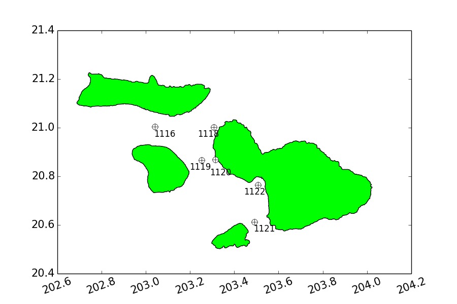
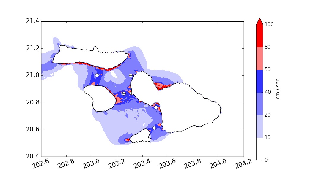
Figure 3: Left: Station locations in the inter-island channels (boxed region of Figure 1). Right: Maximum flow speed from model simulation (scale in cm/s).

The left panel of Figure 3 shows the boxed region from Figure 1 and the stations that lie in the inter-island channels between the islands of Maui, Molokai, and Lanai. The simulations reveal that there is much greater spatial variation in flow speed than is typically observed in sea surface elevation. This makes it potentially more challenging to accurately compute the flow velocity at any particular point. To illustrate this variation, the right panel of Figure 3 shows the maximum computed flow speed $s=\sqrt{u^{2}+v^{2}}$ calculated over the entire 13 hours of simulated time within this region. Note that velocities are much larger between the islands than in the surrounding waters (where tsunami currents are generally less than 10 cm/s), and are largest in the narrowest constrictions between islands, up to 50 cm/s. This is consistent with what is expected from the fluid dynamics and observed in other tsunamis (e.g. Borrero et al (1997); Lynett et al (2012)).

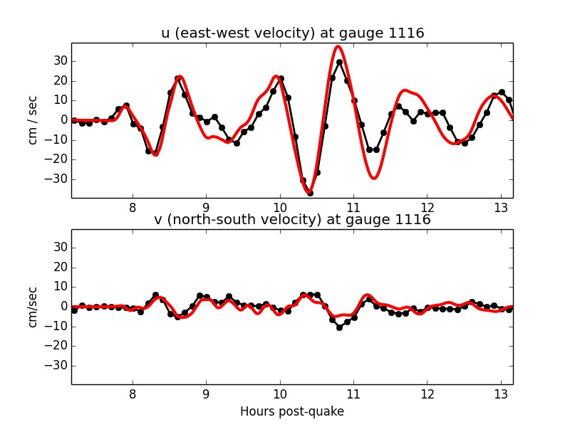
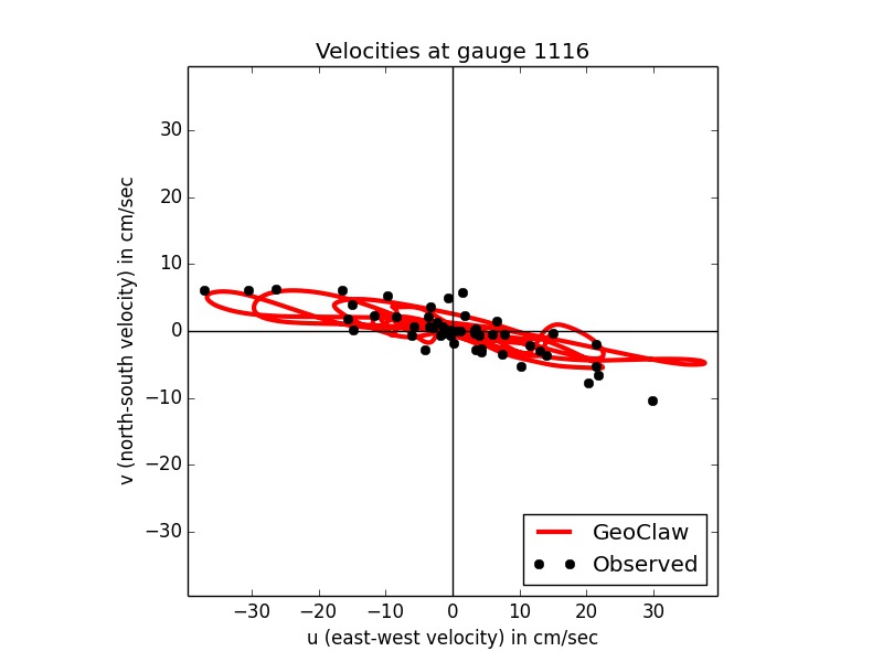
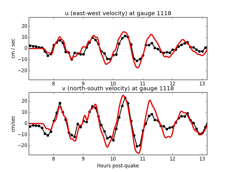
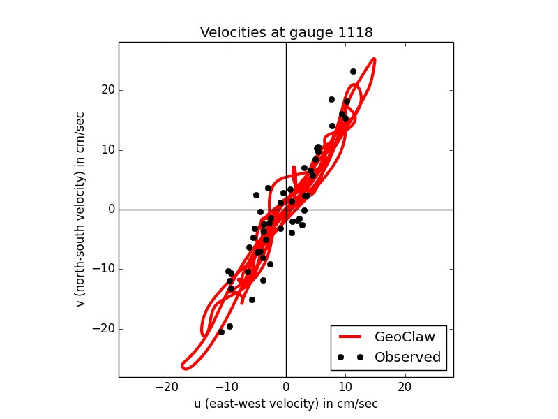
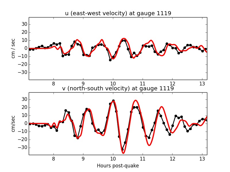
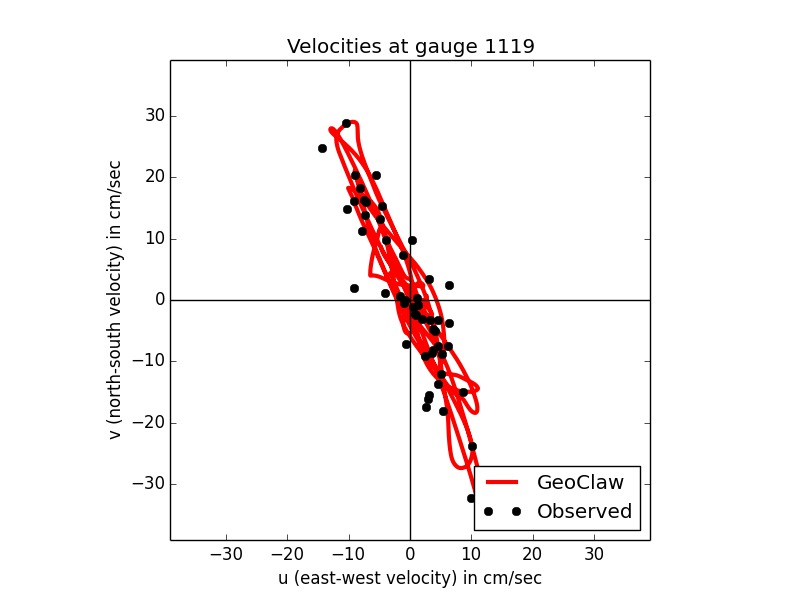
Figure 4: Observed depth-averaged velocity compared to simulated tsunami velocity at each current meter over a 6 hour window at stations HAI1116, 1118, and 1119. Left: $u$ and $v$ components of velocity vs. time. The GeoClaw results (red solid line) have been shifted by +10 minutes in all cases as discussed in the text. Right: Plotted in the $u$–$v$ plane, showing direction of flow.

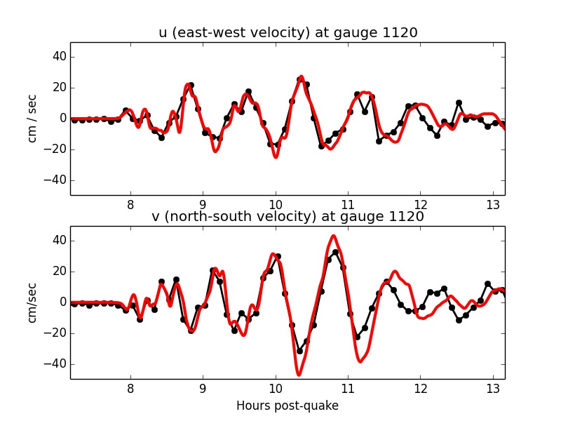
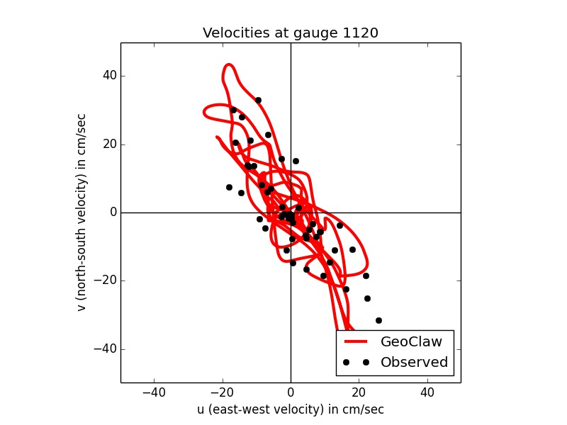
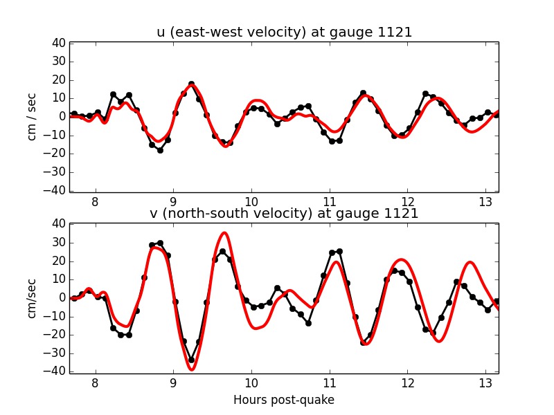
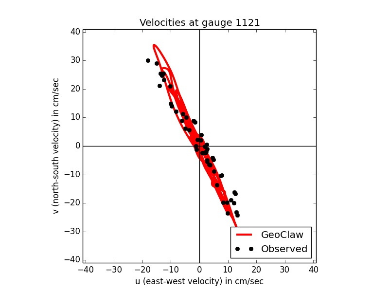
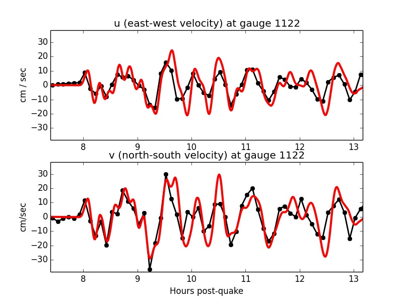
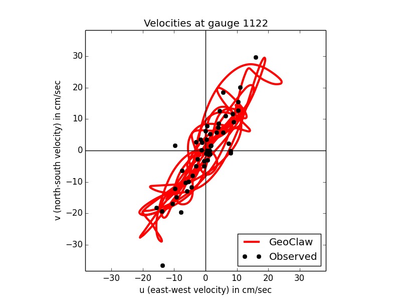
Figure 5: Observed depth-averaged velocity compared to simulated tsunami velocity at each current meter over a 6 hour window at stations HAI1120, 1121, and 1122. See Figure 4 caption for description of plots. plots.

Figures 4 and 5 show the computed flow velocities at the stations in these channels, plotted along with the observations in two different forms. In the left column, the east-west velocity $u$ and north-south velocity $v$ are plotted as time series for roughly 6 hours after the tsunami arrival time. In the right column of each figure we plot both the observed and computed velocities in the $u$–$v$ plane to show the direction of flow. In general, the computed flow direction matches the observed direction quite well, along with the amplitudes. The periods and general wave form are also very similar at almost all these inter-island stations.

We also considered four stations that are in or near harbors: HAI1107 (Honolulu), HAI1123 (Kahului), and HAI1125, HAI1126 (Hilo). The left panel of Figure 6 shows the location of gauge HAI1107 near Honolulu Harbor, along with the tide gauge (TG) where surface elevation data is available. The right panel of Figure 6 shows the maximum speed that was observed over the full simulation at each point in this region.

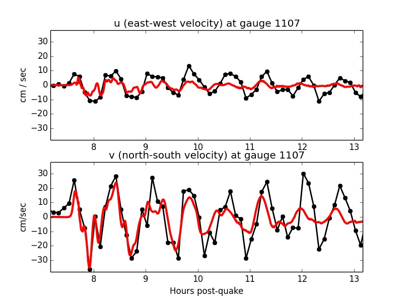
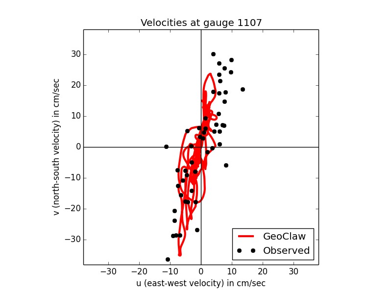
Figure 7: Observed depth averaged velocity compared to simulated tsunami velocity at each current meter over a 6 hour window at station HAI1107. See Figure 4 caption for description of plots.

Figure 7 shows the computed flow velocities at HAI1107, plotted in the same manner as Figures 4 and 5. Again the results agree reasonably well in amplitude, phase and direction, particularly for the first waves.

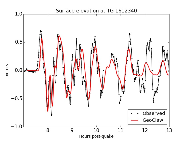
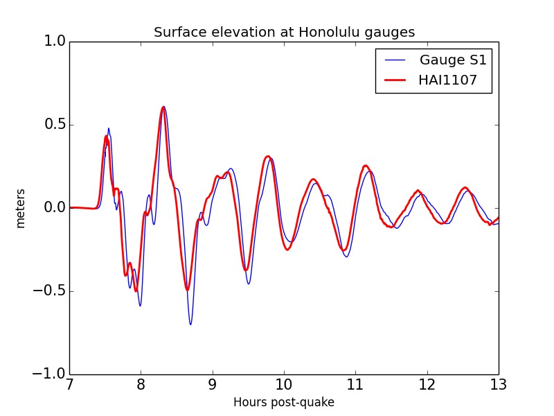
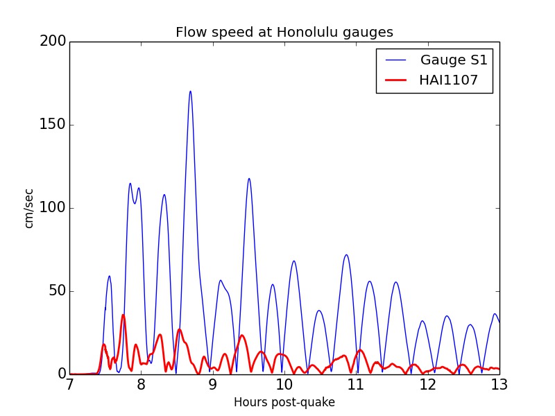
Figure 8: Left: Observed and computed surface elevation at Tide gauge 1612340 Honolulu, Center: Computed surface elevation at HAI1107 and a nearby synthetic gauge S1, Right: Computed flow speed at HAI1107 and a nearby synthetic gauge S1. This figure illustrates that there is much greater spatial variation in velocities than elevation. See Figure 6 for station locations.

The left panel of Figure 8 shows the measured sea surface elevation (after de-tiding as described above) at the tide gauge 1612340, along with the GeoClaw simulation results at the same point. Such comparisons are typical of the manner in which numerical tsunami models have been validated in the past against tide gauge data. The amplitudes and periods match quite well between the observations and computations, at least for the first several waves.

The remaining plots in Figure 8 further illustrate the fact that velocities can exhibit much greater spatial variation than surface elevation. The middle panel of Figure 8 shows computed surface elevations at station HAI1107 and an additional synthetic station marked S1 in Figure 6 that was used in the numerical simulation, located in a dredged ship channel (no observations are available at this point). The time series of surface elevation is virtually identical between these gauges, and they are also similar to the surface elevations at the tide gauge further back in the harbor. On the other hand, the right panel of Figure 8 shows the time series of computed speeds $s=\sqrt{u^{2}+v^{2}}$ at the two locations HAI1107 and S1, and it is seen that the speed varies by more than a factor of 10 and has quite a different temporal pattern. In view of this, we find it particularly notable that the numerical model is able to calculate results that agree as well as they do with observations of velocity at the particular points where the gauges were located.

Figure 6 also shows the location of the Kilo Nalu Observatory marked as KN. Velocity data at a single depth of 12 m at this location are presented in the work of Yamazaki et al (2012), and Figure 3 from that paper shows a maximum flow speed of roughly 25 cm/sec. This is roughly consistent with our figure for the maximum depth-averaged velocity, which shows that this meter was in a region of even lower maximum current velocity than HAI1107.

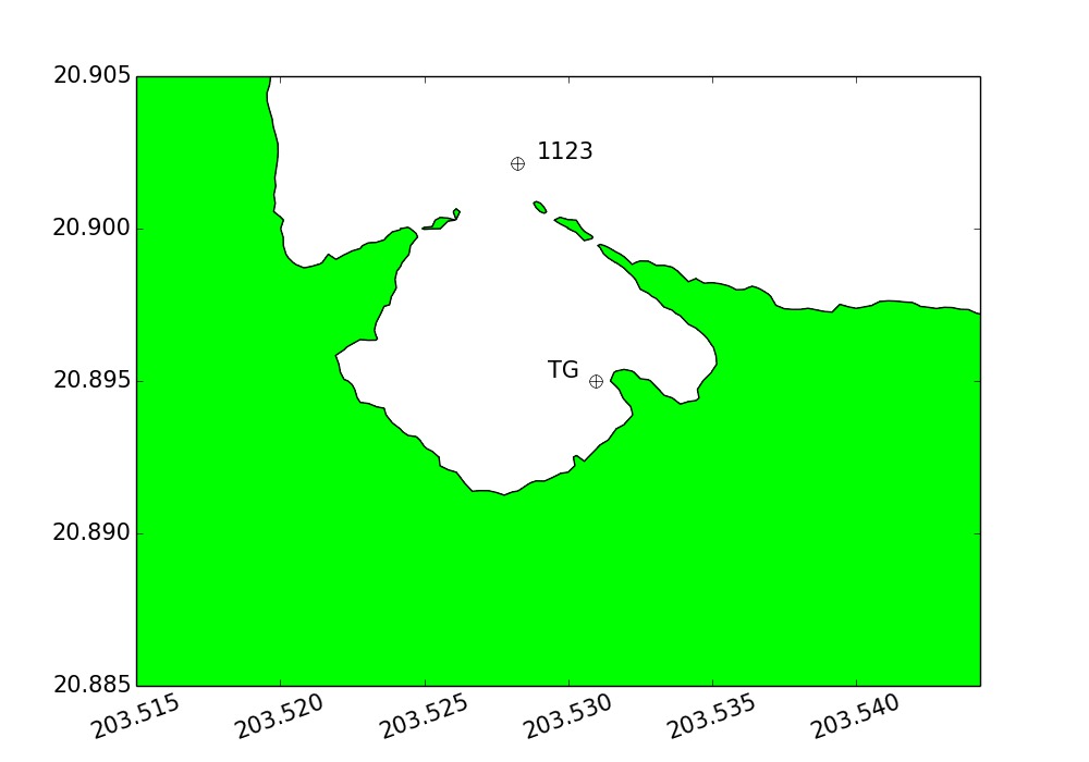
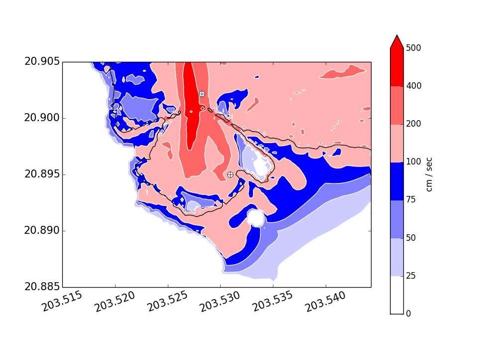
Figure 9: Left: Station locations near Kahului Harbor, including tide gauge 1615680 (TG). Right: Maximum flow speed from model simulation (scale in cm/s).

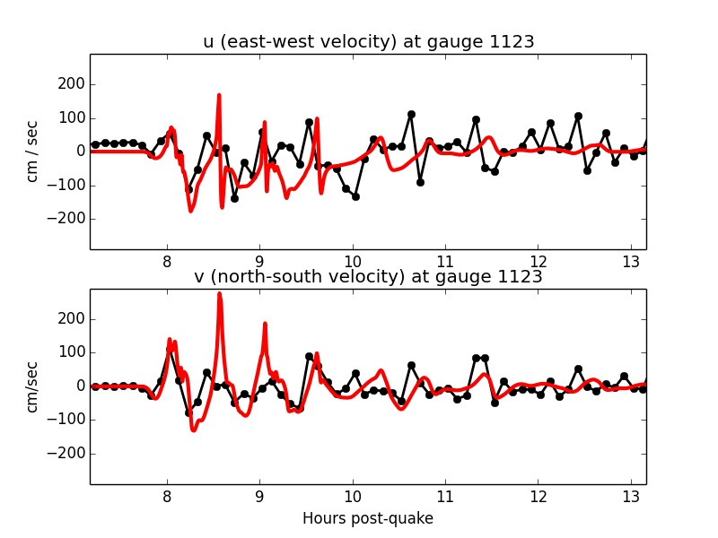
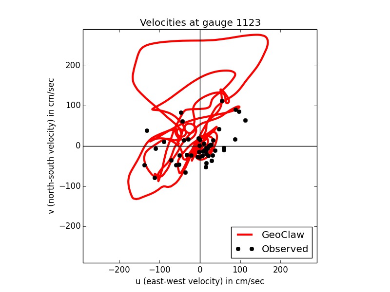
Figure 10: Observed depth-averaged velocity compared to simulated tsunami velocity at each current meter over a 3 hour window at station HAI1123. See Figure 4 caption for description of plots.

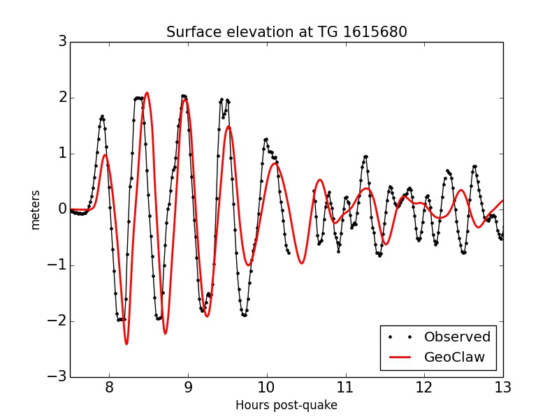
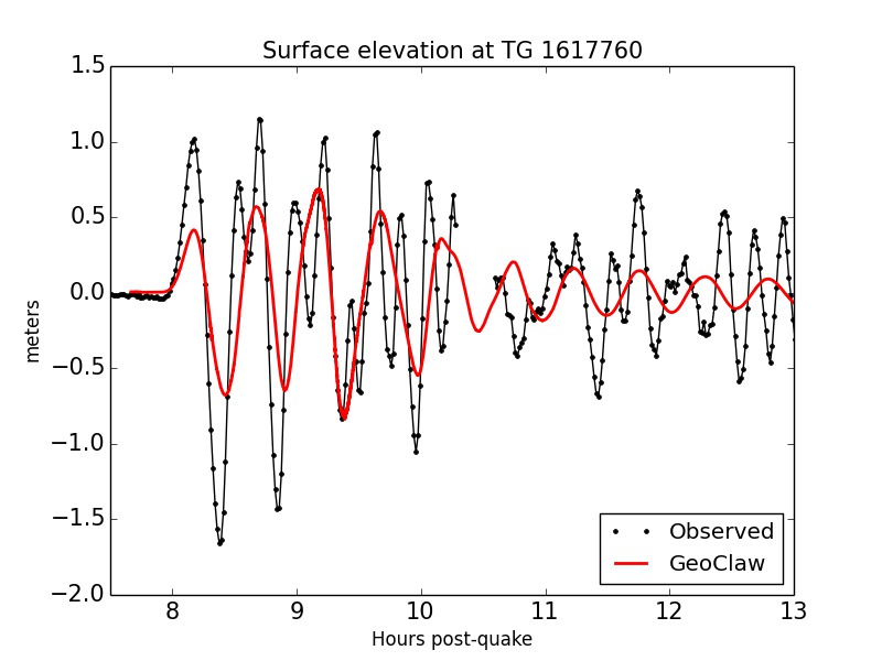
Figure 11: Surface elevation at tide gauges 1615680 Kahului (left) and 1617760 Hilo (right). The GeoClaw results (red solid line) have been shifted by +10 minutes in all cases as discussed in the text.

Station HAI1123 is very close to the entrance to Kahului Harbor. The location is shown in Figure 9, which also illustrates how much spatial variation there is in maximum velocity near this harbor due to the bathymetry. For this harbor only $1^{\prime\prime}$ bathymetry data are available (unlike Honolulu and Hilo Harbors, where $1/3^{\prime\prime}$ bathymetry data have been used). The observations also show a lack of clear directionality, indicating that the flow near the harbor entrance may have been turbulent. In view of these considerations, the relatively poor agreement at HAI1123 in Figure 10 is perhaps not surprising. But note also from Figure 9 that the maximum velocity is very sensitive to the exact position of the gauge and shifting it slightly to the east would give smaller amplitude velocities that might better match the observations. This extreme spatial sensitivity may make it impossible to achieve close agreement, even if the model were perfect, since the location of this gauge is not precisely known. Three digits to the right of the decimal are recorded in the station metadata. Even if all these digits are correct, an uncertainty of $0.0005^{\circ}$ is roughly 50 meters. Figure 11 shows the surface elevation at the tide gauge 1615680 in Kahului Harbor, which shows better agreement than the velocity results in this case.

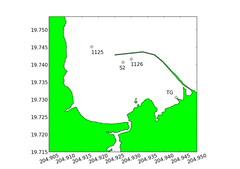
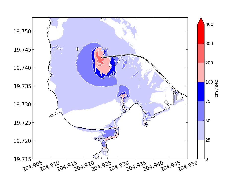
Figure 12: Left: Station locations near Hilo Harbor, including HAI1125, 1126, tide gauge 1617760 (TG), and a synthetic gauge S2. Right: Maximum flow speed from model simulation (scale in cm/s).

Stations HAI1125 and HAI1126 are in the vicinity of Hilo Harbor, as shown in Figure 12 along with tide gauge 1617760. The tsunami currents at HAI1125 are predominantly N–S, both in the observations and the GeoClaw results, as water flows in and out of the harbor. On the other hand the nearby station HAI1126 is very close to the E–W running seawall, and the observed velocities here are more aligned with the seawall. At this station there is not very good agreement between the observations and the computed velocities. There may be several causes for this. Note from the right side of Figure 12 that very high velocities are computed near the end of the seawall. It is also to be expected that strong vorticity is generated as the flow goes around this point and that water will swirl around in the harbor. The perpendicular change in direction between these two nearby stations is further indication that flow inside the harbor is likely to be turbulent. Station HAI1126 is also in quite shallow water (12.46 m) and close to the wall, so we might expect fairly turbulent and perhaps fully three-dimensional fluid behavior near this station that could be strongly affected by small scale bathymetric features. We also note that the tide gauge in this harbor also shows the worst agreement with the computed results (the right panel of Figure 11), further indication that the flow may be too complex to be adequately modeled by the shallow water equations in this harbor.

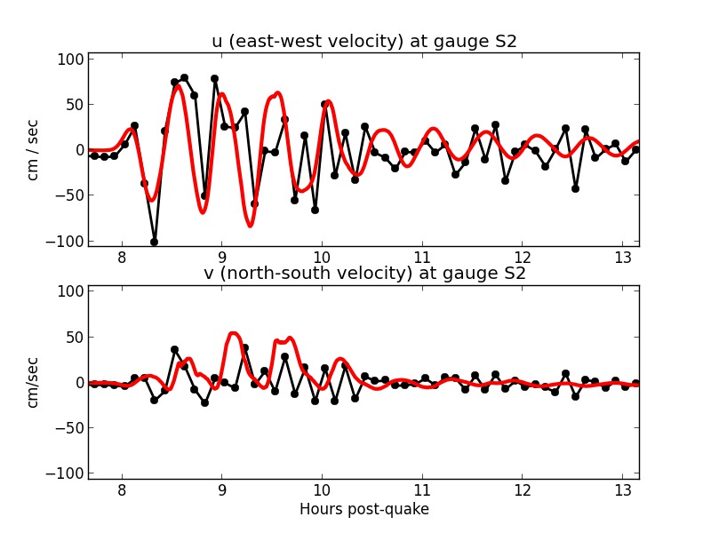
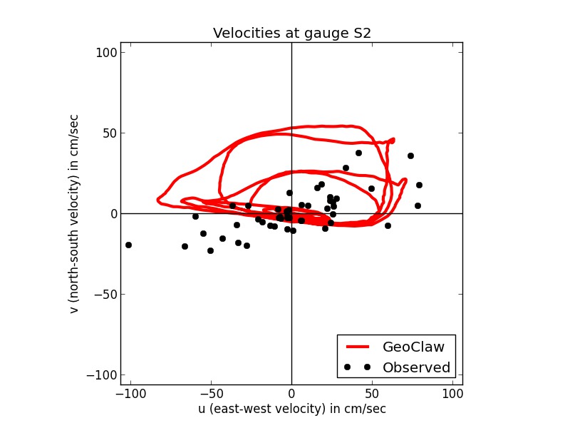
Figure 14: Observed depth-averaged velocity at station HAI1126 compared to simulated tsunami velocity at synthetic gauge location S2 shown in Figure 12.

On the other hand, note that although the computed velocities at the location of HAI1126 are considerably smaller than the observed velocities, there are points nearby where the velocities are comparable. In particular, a gauge placed at the location marked S2 in Figure 12 give the velocity time series shown in Figure 14, which is much more similar to the observations. The S2 gauge is located at $(204.92753,19.74067)$ and is roughly 280 meters from the recorded location of HAI1126.

5 Arrival time

The simulated tsunami generally arrived about 10 minutes before the observed tsunami, roughly 8 hours after the earthquake. This phase shift corresponds to a relative error of about 2% in the velocity of the leading wave. About half of this time difference can be explained quite well by the fact that the linearized shallow water equations are non-dispersive, meaning that the wave speed $\sqrt{gh}$ is independent of the wavelength. The three-dimensional fluid dynamics is better modeled by depth-averaged equations such as Boussinesq or Serre equations that include additional higher order dispersive terms. These terms are generally negligible if the wavelength of the tsunami is very long compared to the depth of the ocean, as is often the case for large-scale tsunamis caused by megathrust earthquakes. However, the Tohoku earthquake had an unusual concentration of slip on a small portion of the fault plane, leading to a tsunami with a relatively short wavelength. The dispersion relation for better models of the fluid dynamics in this situation is often taken to be

$$\omega^{2}=gk\tanh(kh)$$ (3)

(see González and Kulikov (1993)), where $\omega$ is the temporal frequency and $k$ is the spatial wave number, given by $k=2\pi/L$ in terms of the wavelength $L$. The depth of the ocean $h$ is assumed constant in this analysis. From this dispersion relation it can be shown that the group velocity $d\omega/dk$ for wavenumber $k$ can be expanded as

$$\omega^{\prime}(k)=\sqrt{gh}\left(1-\frac{1}{2}k^{2}h^{2}+{\cal O}(k^{4}h^{4})\right).$$ (4)

Estimating an average ocean depth of 4500 m (based on the travel time between the source region and Hawaii) and a wavelength of roughly 200 km from ocean-scale plots of the solution, we obtain $\frac{1}{2}k^{2}h^{2}\approx 0.01$, which would result in about a 1% change in the arrival time of the wave, or about 5 minutes. The remaining 5 minute time shift has also been observed by other researchers modeling results in Hawaii using dispersive Boussinesq equations (Kirby et al (2013); Yamazaki et al (2012)). At least part of it is due to the use of an instantaneous displacement of the sea surface at the initiation time of the earthquake, as has been used in this study and is standard practice in tsunami modeling, rather than modeling the dynamic seafloor motion and delayed response of the sea surface. Additional discrepancies may have resulted from dispersion due to the effects of ocean or tidal currents not modeled numerically.

6 Discussion and conclusions

Recorded observations in many locations show velocities that are not uniform in the water column. This may bring into question the suitability of the shallow water equations for modeling such flows. We believe our results show that in fact the depth averaged equations can often be successfully used, even for locations such as gauge HAI1119 where Figure 2 shows that there is significant variation with depth and yet Figure 4 shows good agreement of the average velocity with the shallow water equation results. It should also be noted that there appears to be less variation with depth of the velocity in Figure 2 after the tsunami arrives than before, and hence the tsunami current may be more vertically uniform than the ambient currents. This is an important issue that deserves further study.

The high spatial variability of the tsunami current velocities makes it potentially much more challenging to accurately model velocities at specific locations than to capture surface elevation. Differences in the location and timing of maximum tsunami elevation and velocity has been shown in other studies (e.g. González et al (2009)). In view of this we believe the agreement seen between the GeoClaw simulations and the observations at most of the stations studied provides significant additional validation of the model beyond what has been achieved by past studies.

Model results and observations differed the most at stations HAI1123 and HAI1126, in Kahalui and Hilo Harbors, respectively. We have discussed a number of possible reasons, including the lack of sufficiently accurate bathymetry and fact that flows are expected to be much more complex and perhaps more three-dimensional and turbulent inside harbors. Moreover the extreme sensitivity of the velocity to spatial location and the uncertainty in the precise gauge locations may limit the degree to which tsunami models can be quantitatively validated using these observations.

When Figures 6, 9, and 12 are compared, it is evident that the location of highest velocity is highly dependent on harbor configuration. The harbors of Honolulu, Hilo and Kahului experience maximum velocities in different settings within the harbor. In Honolulu Harbor, which has a broad entrance, the maximum velocities are simulated in a broad zone near the harbor entrance and within smaller channels. In Kahului Harbor, which has a narrow entrance, the maximum velocities are simulated in a swath perpendicular to the harbor entrance with lower velocities along the edges of the harbor. In Hilo Harbor, the highest velocities are simulated at the end of the seawall. Other studies have shown alterations to harbor shape and bathymetry can change tsunami behavior (Dengler and Uslu (2011)).

An important future direction in tsunami modeling is the simulation of sediment transport. The capability to model both tsunami erosion and deposition will aid in hazard analysis and is also a crucial tool in helping to reconstruct past events from tsunami deposits. Accurate sediment transport simulations require that numerical models produce accurate fluid velocities and accelerations, giving additional impetus to validate codes against real-world data sets such as the ones used here.

The greater spatial variability in tsunami velocity than wave height has implications for future sediment transport studies. The greater variability in velocities is likely a result of the behavior of the flow as it is channelized and as it flows around bathymetric highs and structures. For example, channelized flows between islands and through harbor entrance are high as are flows around projecting features such as the seawall in Hilo Harbor. Wave height does not respond as strongly to channelized flow as current velocity. This indicates that sediment is likely not uniformally eroded at vaious water depths but erosion is concentrated in locations of higher flow velocities. High-resolution bathymetry will be necessary to accurately model sediment erosion for tsunami models.

This work focused on stations near harbors and those within the channels between the islands of Maui, Molokai, and Lanai, where there is a persistent tsunami signal due to the seiching of water in these protected regions. The stations not studied in this work were in less protected settings. We have not yet investigated all of them, but in preliminary studies the numerical simulations did not match the observations as well at some of the other sites. Stronger and more erratic background currents at these stations play a role. In addition, we believe that reflections from distant bathymetric features may be much more important in the observed tsunami signal at these points, and that additional refinement over a larger portion of the ocean may be required in the future study of these stations.

All data and computer code used in this study (both the GeoClaw simulation code and the analysis code) is available via the Github repository
        https://github.com/rjleveque/tohoku2011-paper2.
We hope that the data available from these velocity meters will also be used as benchmark tests for other tsunami simulation codes in the future.

7 Acknowledgments

The authors are grateful to SeanPaul La Selle for assistance in acquiring and processing the data. This research was supported in part by NSF Grants DMS-0914942 and DMS-1216732, NSF RAPID Grant DMS-1137960, the Founders Term Professorship in Applied Mathematics at the University of Washington.

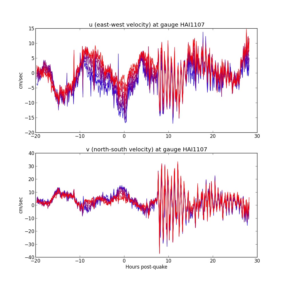
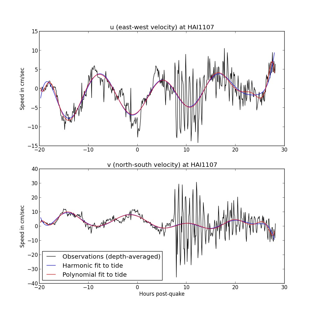
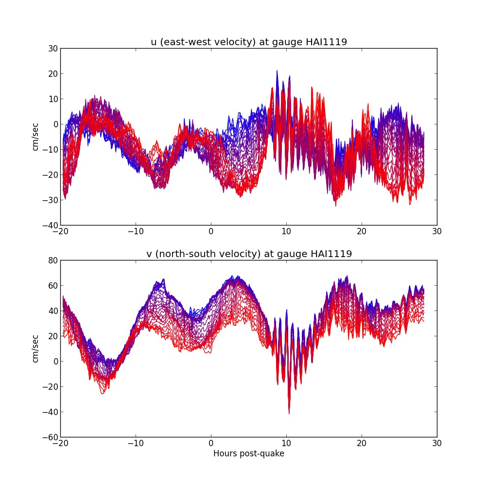
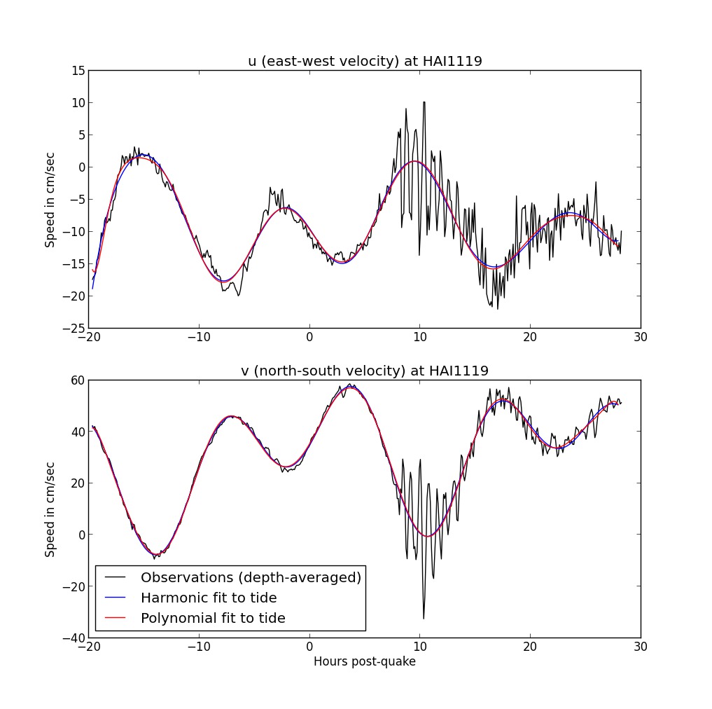
Figure 2: Plots of observed velocities at two sample stations, HAI1107, Honolulu Harbor, and HAI1119, Auau Channel. On the left, velocities are shown at all depths, split into u and v velocity components. Blue is the shallower gauges, Red is the deeper gauges. On the right, the depth averaged velocities are shown in black and the tidal component based on harmonic constituents is shown in blue. Also shown in red is a polynomial fit to the tidal component. In subsequent figures the tidal component as determined by the harmonic fit is subtracted from the data. Shown over a 48-hour window around the tsunami arrival time at roughly 8 hours post-quake.

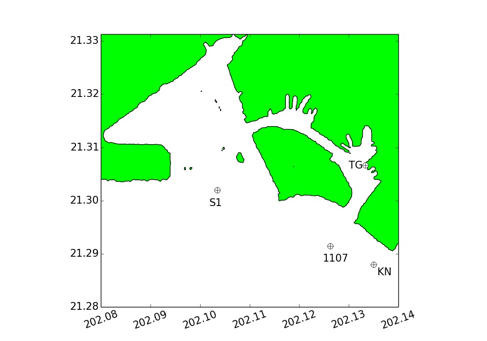
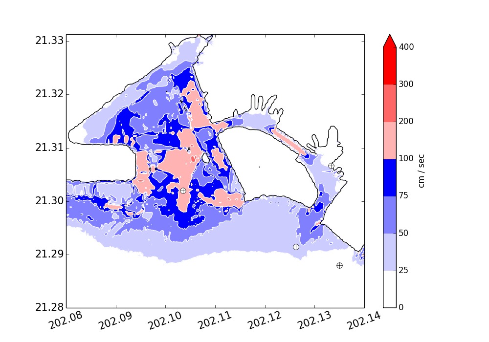
Figure 6: Left: Station locations near Honolulu Harbor, including HAI1107, tide gauge 1612340 (TG), a synthetic gauge (S1), and the Kilo Nalu Observatory (KN). Right: Maximum flow speed from model simulation (scale in cm/s).

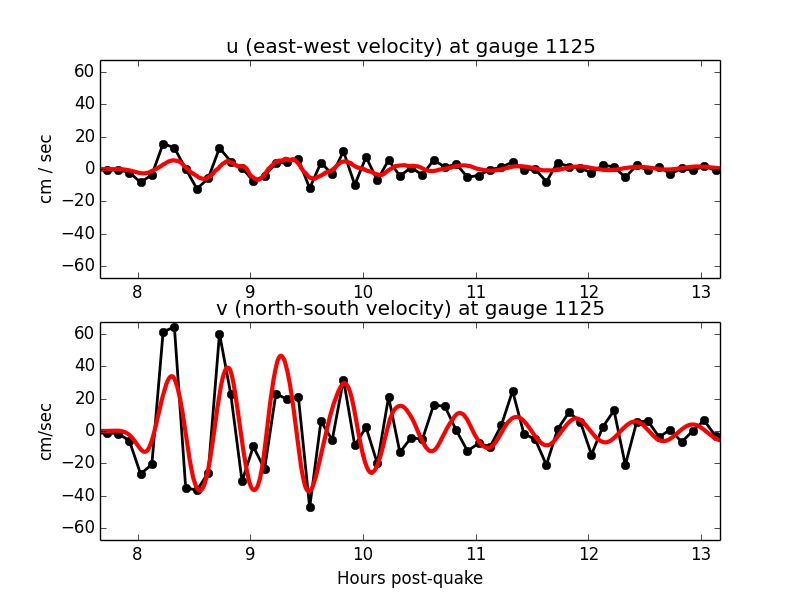
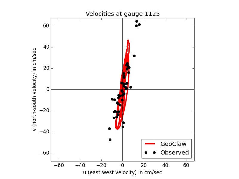
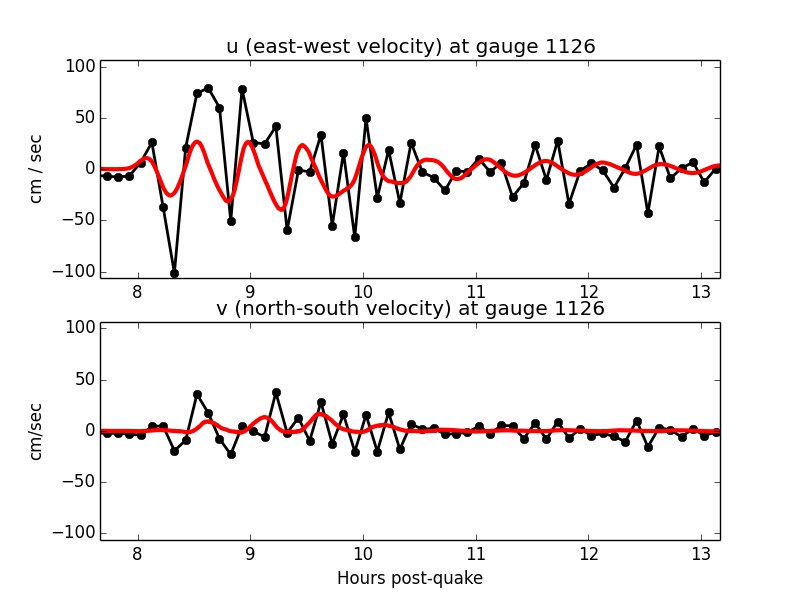
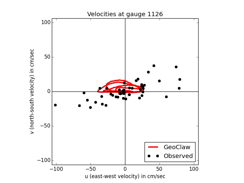
Figure 13: Observed depth-averaged velocity compared to simulated tsunami velocity at each current meter over a 6 hour window at stations HAI1125 and 1126. See Figure 4 caption for description of plots.

References

- Admire et al (2011) Admire A, Dengler L, Crawford G, Uslu B, Montoya J, Wilson R (2011) Observed and modeled tsunami currents on California’s north coast. In: American Geophysical Union, Fall Meeting 2011, pp #NH14A–03
- Admire (2013) Admire AR (2013) Observed and modeled tsunami currents on California’s north coast. Master’s thesis, Humboldt State University
- Admire et al (2014) Admire AR, Dengler LA, Crawford GB, Uslu BU, Borrero JC, Greer SD, Wilson RI (2014) Observed and modeled currents from the tohoku-oki, japan and other recent tsunamis in northern california. Pure and Applied Geophysics DOI 10.1007/s00024-014-0797-8, URL http://link.springer.com/10.1007/s00024-014-0797-8
- Amante and Eakins (2009) Amante C, Eakins B (2009) ETOPO1 1 arc-minute global relief model: Procedures, data sources and analysis. NOAA Technical Memorandum NESDIS NGDC-24 p 19
- Apotsos et al (2011) Apotsos A, Buckley M, Gelfenbaum G, Jaffe B, Vatvani D (2011) Nearshore tsunami inundation model validation: Toward sediment transport applications. Pure and Applied Geophysics 168(11):2097–2119
- Arcas and Wei (2011) Arcas D, Wei Y (2011) Evaluation of velocity-related approximations in the non-linear shallow water equations for the Kuril Islands, 2006 tsunami event at Honolulu, Hawaii. Geophys Res Lett 38:doi: 10.1029/2011GL047,083
- Berger et al (2011) Berger MJ, George DL, LeVeque RJ, Mandli KT (2011) The GeoClaw software for depth-averaged flows with adaptive refinement. Adv Water Res 34:1195–1206, URL www.clawpack.org/links/papers/awr11
- Borrero et al (1997) Borrero J, Ortiz M, Titov V, Synolakis C (1997) Field survey of Mexican tsunami produces new data, unusual photos. EOS 78:85, 87–89
- Bourgeois (2009) Bourgeois J (2009) Geologic effects and records of tsunamis. In: Bernard EN, Robinson AR (eds) The Sea, Harvard University Press, vol 15, pp 55–92
- Bretschneider et al (1986) Bretschneider CL, Krock HJ, Nakazaki E, Casciano FM (1986) Roughness of typical Hawaiian terrain for tsunami run-up calculations: A user’s manual. J.K.K. Look Laboratory Report, University of Hawaii, Honolulu
- Bricker et al (2007) Bricker JD, Munger S, Pequignet C, Wells JR, Pawlak G, Cheung KF (2007) ADCP observations of edge waves off Oahu in the wake of the November 2006 Kuril Islands tsunami. Geophysical Research Letters 34(23), DOI 10.1029/2007GL032015, URL http://dx.doi.org/10.1029/2007GL032015
- Cheung et al (2013) Cheung KF, Bai Y, Yamazaki Y (2013) Surges around the Hawaiian islands from the 2011 Tohoku tsunami. J Geophys Res 118:5703–5719, DOI 10.1002/jgrc.20413, URL http://onlinelibrary.wiley.com/doi/10.1002/jgrc.20413/abstract
- Co-Ops Survey (Accessed 23 September 2011) Co-Ops Survey (Accessed 23 September 2011) Historic Current Survey Data, National Atmospheric and Oceanic Administration. URL http://tidesandcurrents.noaa.gov/cdata/StationList?type=Current%20Data&filter=survey
- Dao and Tkalich (2007) Dao MH, Tkalich P (2007) Tsunami propagation modelling — a sensitivity study. Natural Hazards and Earth System Science 7(6):741–754, DOI 10.5194/nhess-7-741-2007, URL http://www.nat-hazards-earth-syst-sci.net/7/741/2007/
- Dengler and Uslu (2011) Dengler L, Uslu B (2011) Effects of harbor modification on Crescent City, California’s tsunami vulnerability. Pure and Applied Geophysics 168:1175–1185, URL http://dx.doi.org/10.1007/s00024-010-0224-8, 10.1007/s00024-010-0224-8
- Earthquake Engineering Research Institute (2011) Earthquake Engineering Research Institute (2011) The Tohoku, Japan, Tsunami of March 11, 2011: Effects on Structures. URL https://www.eeri.org
- Flament et al (1996) Flament P, Kennan S, Lumpkin R, Sawyer M, Stroup E (1996) The Ocean Atlas of Hawai’i. URL http://oos.soest.hawaii.edu/pacioos/outreach/oceanatlas/
- Fritz et al (2011) Fritz H, Petroff C, Catalán P, Cienfuegos R, Winckler P, Kalligeris N, Weiss R, Barrientos S, Meneses G, Valderas-Bermejo C, Ebeling C, Papadopoulos A, Contreras M, Almar R, Dominguez J, Synolakis C (2011) Field survey of the 27 February 2010 Chile tsunami. Pure and Applied Geophysics 168:1989–2010, URL http://dx.doi.org/10.1007/s00024-011-0283-5, 10.1007/s00024-011-0283-5
- Fritz et al (2006) Fritz HM, Borrero JC, Synolakis CE, Yoo J (2006) 2004 Indian Ocean tsunami flow velocity measurements from survivor videos. Geophys Res Lett 33:10.1029/2006GL026,784
- Fritz et al (2012) Fritz HM, Phillips DA, Okayasu A, Shimozono T, Liu H, Mohammed F, Skanavis V, Synolakis CE, Takahashi T (2012) The 2011 Japan tsunami current velocity measurements from survivor videos at Kesennuma Bay using LiDAR. Geophys Res Lett 39:doi:10.1029/2011GL050,686
- Fujii et al (2011) Fujii Y, Satake K, Sakai S, Shinohara M, Kanazawa T (2011) Tsunami source of the 2011 off the Pacific coast of Tohoku earthquake. Earth Planets Space 63:815–820
- GeoClaw authors (2012) GeoClaw authors (2012) GeoClaw software, version 4.6.2. URL http://www.clawpack.org/geoclaw
- George (2006) George DL (2006) Finite volume methods and adaptive refinement for tsunami propagation and inundation. PhD thesis, University of Washington
- George (2008) George DL (2008) Augmented Riemann solvers for the shallow water equations over variable topography with steady states and inundation. J Comput Phys 227:3089–3113
- George and LeVeque (2006) George DL, LeVeque RJ (2006) Finite volume methods and adaptive refinement for global tsunami propagation and local inundation. Science of Tsunami Hazards 24:319–328
- González et al (2011) González F, LeVeque RJ, Varkovitzky J, Chamberlain P, Hirai B, George DL (2011) GeoClaw Results for the NTHMP Tsunami Benchmark Problems. http://www.clawpack.org/links/nthmp-benchmarks/geoclaw-results.pdf
- González and Kulikov (1993) González FI, Kulikov YA (1993) Tsunami dispersion observed in the deep ocean. In: Tinti S (ed) Tsunamis in the World, Kluwer Academic Publishers, Advances in Natural and Technological Hazards Research, vol 1, pp 7–16
- González et al (2009) González FI, Geist EL, Jaffe B, Kânoglu U, Mofjeld H, Synolakis CE, Titov VV, Arcas D, Bellomo D, Carlton D, Horning T, Johnson J, Newman J, Parsons T, Peters R, Peterson C, Priest G, Venturato A, Weber J, Wong F, Yalciner A (2009) Probabilistic tsunami hazard assessment at Seaside, Oregon, for near- and far-field seismic sources. Journal of Geophysical Research: Oceans 114:C11,023, DOI 10.1029/2008JC005132, URL http://dx.doi.org/10.1029/2008JC005132
- Huntington et al (2007) Huntington K, Bourgeois J, Gelfenbaum G, Lynett P, Jaffe B, Yeh H, Weiss R (2007) Sandy signs of a tsunami’s onshore depth and speed. EOS 88:577–578, URL http://www.agu.org/journals/eo/eo0752/2007EO52_tabloid.pdf
- Jaffe and Gelfenbaum (2007) Jaffe BE, Gelfenbaum G (2007) A simple model for calculating tsunami flow speed from tsunami deposits. Sedimentary Geology 3-4:347–361
- Kirby et al (2013) Kirby JT, Shi F, Tehranirad B, Harris JC, Grilli ST (2013) Dispersive tsunami waves in the ocean: model equations and sensitivity to dispersion and Coriolis effects. Ocean Modeling 62:39–55
- Lacy et al (2012) Lacy J, Rubin D, Buscombe D (2012) Currents, drag, and sediment transport induced by a tsunami. Journal of Geophysical Research 117, DOI 10.1029/2012JC007954
- LeVeque (2002) LeVeque RJ (2002) Finite Volume Methods for Hyperbolic Problems. Cambridge University Press, URL http://amath.washington.edu/ claw/book.html
- LeVeque and George (2007) LeVeque RJ, George DL (2007) High-resolution finite volume methods for the shallow water equations with bathymetry and dry states. In: Liu PLF, Yeh H, Synolakis C (eds) Advanced Numerical Models for Simulating Tsunami Waves and Runup, vol 10, pp 43–73, URL http://www.amath.washington.edu/ rjl/pubs/catalina04/
- LeVeque et al (2011) LeVeque RJ, George DL, Berger MJ (2011) Tsunami modeling with adaptively refined finite volume methods. Acta Numerica pp 211–289
- Liu et al (2005) Liu PLF, Lynett P, Fernando H, Jaffe BE, Fritz H, Higman B, Morton R, Goff J, Synolakis C (2005) Observations by the International Tsunami Survey Team in Sri Lanka. Science 308(5728):1595
- Lynett et al (2012) Lynett PJ, Borrero JC, Weiss R, Son S, Greer D, Renteria W (2012) Observations and modeling of tsunami-induced currents in ports and harbors. Earth Planet Sci Lett 327-328:68 – 74, DOI 10.1016/j.epsl.2012.02.002
- Lynett et al (2014) Lynett PJ, Borrero J, Son S, Wilson R, Miller K (2014) Assessment of the tsunami-induced current hazard: Lynett et al.: Tsunami-induced current hazard. Geophysical Research Letters pp n/a–n/a, DOI 10.1002/2013GL058680, URL http://doi.wiley.com/10.1002/2013GL058680
- MacInnes et al (2009) MacInnes BT, Pinegina TK, Bourgeois J, Razhigaeva NG, Kaistrenko VM, Kravchunovskaya EA (2009) Field survey and geological effects of the 15 November 2006 Kuril tsunami in the middle Kuril Islands. In: Cummins PR, Satake K, Kong LSL (eds) Tsunami Science Four Years after the 2004 Indian Ocean Tsunami, Pageoph Topical Volumes, Birkhäuser Basel, pp 9–36
- MacInnes et al (2013) MacInnes BT, Gusman AR, LeVeque RJ, Tanioka Y (2013) Comparison of earthquake source models for the 2011 Tohoku event using tsunami simulation and near field observations. Bulletin of the Seismological Society of America 103:1256–1274
- Moore et al (2007) Moore AL, McAdoo BG, Ruffman A (2007) Landward fining from multiple sources in a sand sheet deposited by the 1929 Grand Banks tsunami, Newfoundland. Sedimentary Geology 200(3-4):336–346
- National Geophysical Data Center (Accessed 17 February 2012) National Geophysical Data Center (Accessed 17 February 2012) National Geophysical Data Center, National Atmospheric and Oceanic Administration. URL http://www.ngdc.noaa.gov/dem/squareCellGrid/search
- Okal et al (2010) Okal EA, Fritz HM, Synolakis CE, Borrero JC, Weiss R, Lynett PJ, Titov VV, Foteinis S, Jaffe BE, Lui PLF, Chan I (2010) Field survey of the Samoa tsunami of 29 September 2009. Seismological Research Letters 81:577–591
- Satake et al (2006) Satake K, Aung TT, Sawai Y, Sawai Y, Okamura Y, Win KS, Swe W, Swe C, Swe TL, Tun ST, Soe MM, Oo TZ, Zaw SH (2006) Tsunami heights and damage along the Myanmar coast from the December 2004 Sumatra-Andaman earthquake. Earth, Planet and Space 58:243–252
- Sawai et al (2009) Sawai Y, Jankaew K, Martin ME, Prendergast A, Choowong M, Charoentitirat T (2009) Diatom assemblages in tsunami deposits associated with the 2004 Indian Ocean tsunami at Phra Thong Island, Thailand. Marine Micropaleontology 73(1-2):70–79
- Synolakis and Okal (2005) Synolakis CE, Okal EA (2005) 1992–2002: Perspective on a decade of post-tsunami surveys. Advances in Natural and Technological Hazards Research 23:1–29
- Synolakis et al (2007) Synolakis CE, Bernard EN, Titov VV, Kanoglu U, González FI (2007) Standards, criteria, and procedures for NOAA evaluation of tsunami numerical models. NOAA Tech Memo OAR PMEL-135 p 55
- Tang et al (2009) Tang L, Titov VV, Chamberlain CD (2009) Development, testing, and applications of site-specific tsunami inundation models for real-time forecasting. Journal of Geophysical Research 114:C12,025
- The Western States Seismic Policy Council (2011) The Western States Seismic Policy Council (2011) A perspective from state and territory tsunami programs in the high tsunami risk Pacific region. The Western States Seismic Policy Council Report 2011-01:30
- Weiss (2008) Weiss R (2008) Sediment grains moved by passing tsunami waves: Tsunami deposits in deep water. Mar Geol 250:251–257
- Yamazaki et al (2012) Yamazaki Y, Cheung KF, Pawlak G, Lay T (2012) Surges along the Honolulu coast from the 2011 Tohoku tsunami. Geophysical Research Letters 39(9):L09,604, DOI 10.1029/2012GL051624, URL http://dx.doi.org/10.1029/2012GL051624