Loss of ellipticity for non-coaxial plastic deformations in additive logarithmic finite strain plasticity

Abstract

In this paper we consider the additive logarithmic finite strain plasticity formulation from the view point of loss of ellipticity in elastic unloading. We prove that even if an elastic energy $F\mapsto W(F)=\widehat{W}(\log U)$ defined in terms of logarithmic strain $\log U$, where $U=\sqrt{F^{T}\,F}$, happens to be everywhere rank-one convex as a function of $F$, the new function $F\mapsto\widetilde{W}(F)=\widehat{W}(\log U-\log U_{p})$ need not remain rank-one convex at some given plastic stretch $U_{p}$ (viz. $E_{p}^{\log}:=\log U_{p}$). This is in complete contrast to multiplicative plasticity (and infinitesimal plasticity) in which $F\mapsto W(F\,F_{p}^{-1})$ remains rank-one convex at every plastic distortion $F_{p}$ if $F\mapsto W(F)$ is rank-one convex ($\nabla u\mapsto\|{\rm sym}\nabla u-\varepsilon_{p}\|^{2}$ remains convex). We show this disturbing feature of the additive logarithmic plasticity model with the help of a recently introduced family of exponentiated Hencky energies.

Key words: Hencky strain, logarithmic strain, natural strain, true strain, Hencky energy, multiplicative decomposition, elasto-plasticity, ellipticity domain, isotropic formulation, additive plasticity.

1 Introduction

Geometrically nonlinear plasticity is a field of intensive ongoing research. There exist several fundamentally different approaches which reduce, more or less, to the infinitesimal model based on the additive split of the infinitesimal strain tensor $\varepsilon={\rm sym}\nabla u$ into symmetric elastic and plastic strains [53, 62, 50, 52] $\varepsilon=\varepsilon_{e}+\varepsilon_{p}$. We assume the reader to be familiar with the general framework of finite strain plasticity models.

The involved nonlinearities make it difficult, both from an analysis and algorithmic point of view to obtain definitive results. There exists, however, one well known and much used methodology to reduce the algorithmic complexity dramatically. It is based on the matrix-logarithm and the introduction of a so called plastic metric $C_{p}\in{\rm PSym}(3)$ together with an additive ansatz for elastic strains $E_{e}=\log C-\log C_{p}$. We refer to these models as additive logarithmic. Within these, basically the small strain linearized framework is simply lifted to the geometrically nonlinear setting through the properties of the logarithm. Thus, frame-indifference, thermodynamical admissibility, plastic volume constraint, associative flow rule, principle of maximal dissipation etc. are all easily satisfied.

In this paper, however, we want to exhibit a major drawback of this approach which makes the additive logarithmic ansatz in our view inadmissible in those cases where large plastic deformations need to be considered, as are encountered e.g. in elastic spring back processes in the automobile industry. Without loss of generality, we will concentrate our exposition to the completely isotropic setting, in which most prominently the quadratic Hencky-logarithmic strain energy appears.

1.1 Notation

For $a,b\in\mathbb{R}^{n}$ we let $\langle{a},{b}\rangle_{\mathbb{R}^{n}}$ denote the scalar product on $\mathbb{R}^{n}$ with associated vector norm $\|a\|_{\mathbb{R}^{n}}^{2}=\langle{a},{a}\rangle_{\mathbb{R}^{n}}$. We denote by $\mathbb{R}^{n\times n}$ the set of real $n\times n$ second order tensors, written with capital letters. The standard Euclidean scalar product on $\mathbb{R}^{n\times n}$ is given by $\langle{X},{Y}\rangle_{\mathbb{R}^{n\times n}}=\textrm{tr}{(XY^{T})}$, and thus the Frobenius tensor norm is $\|{X}\|^{2}=\langle{X},{X}\rangle_{\mathbb{R}^{n\times n}}$. In the following we do not adopt any summation convention and we omit the subscript $\mathbb{R}^{n\times n}$ in writing the Frobenius tensor norm. The identity tensor on $\mathbb{R}^{n\times n}$ will be denoted by ${\boldsymbol{\mathbbm{1}}}$, so that $\textrm{tr}{(X)}=\langle{X},{{\boldsymbol{\mathbbm{1}}}}\rangle$, while $\operatorname{dev}_{n}X=X-\frac{1}{n}\,\textrm{tr}(X)\cdot{\boldsymbol{\mathbbm{1}}}$ is the n-dimensional deviatoric part of a second order tensor $X{\in\mathbb{R}^{n\times n}}$. We let $\operatorname{Sym}(n)$ and ${\rm PSym}(n)$ denote the symmetric and positive definite symmetric tensors respectively. We adopt the usual abbreviations of Lie-group theory, i.e., ${\rm GL}(n):=\{X\in\mathbb{R}^{n\times n}\;|\det{X}\neq 0\}$ denotes the general linear group, ${\rm SL}(n):=\{X\in{\rm GL}(n)\;|\det{X}=1\},\;\mathrm{O}(n):=\{X\in{\rm GL}(n)\;|\;X^{T}X={\boldsymbol{\mathbbm{1}}}\},\;{\rm SO}(n):=\{X\in{\rm GL}(n,\mathbb{R})\;|X^{T}X={\boldsymbol{\mathbbm{1}}},\;\det{X}=1\}$, ${\rm GL}^{+}(n):=\{X\in\mathbb{R}^{n\times n}\;|\det{X}>0\}$ is the group of invertible matrices with positive determinant, $\mathfrak{so}(3):=\{X\in\mathbb{R}^{3\times 3}\;|X^{T}=-X\}$ is the Lie-algebra of skew symmetric tensors and $\mathfrak{sl}(3):=\{X\in\mathbb{R}^{3\times 3}\;|\textrm{tr}({X})=0\}$ is the Lie-algebra of traceless tensors. For $X\in{\rm PSym}(n)$, $X=\sum_{i=1}^{n}\lambda_{i}\,N_{i}\otimes N_{i}$, where $\lambda_{i}$ are the eigenvalues and $N_{i}$ are the eigenvectors of $X$, we consider $\log X=\sum_{i=1}^{n}\log\lambda_{i}(N_{i}\otimes N_{i})$. Here and in the following the superscript ^T is used to denote transposition. For all vectors $\xi,\eta\in\mathbb{R}^{3}$ we have the (dyadic) tensor product $(\xi\otimes\eta)_{ij}=\xi_{i}\,\eta_{j}$. The set of positive real numbers is denoted by $\mathbb{R}_{+}:=(0,\infty)$, while $\overline{\mathbb{R}}_{+}{:}=\mathbb{R}_{+}\cup\{\infty\}$.

Let us consider $W(F)$ to be the strain energy function of an elastic material in which $F=\nabla\varphi$ is the gradient of a deformation from a reference configuration to a configuration in the Euclidean 3-space; $W(F)$ is measured per unit volume of the reference configuration. The domain of $W(\cdot)$ is ${\rm GL}^{+}(n)$. We denote by $C=F^{T}F$ the right Cauchy-Green strain tensor, by $B=F\,F^{T}$ the left Cauchy-Green (or Finger) strain tensor, by $U=\sqrt{F^{T}F}$ the right stretch tensor, i.e., the unique element of ${\rm PSym}(n)$ for which $U^{2}=C$ and by $V$ the left stretch tensor, i.e., the unique element of ${\rm PSym}(n)$ for which $V^{2}=B$. Here, we are only concerned with rotationally symmetric functions (objective and isotropic), i.e., $W(F)={W}(Q_{1}^{T}\,F\,Q_{2})\ \forall\,F=R\,U=VR\in{\rm GL}^{+}(n),\ Q_{1},Q_{2},R\in{\rm SO}(n).$ We denote by $S_{1}=D_{F}[W(F)]$ the first Piola-Kirchhoff stress tensor and by $\sigma=\frac{1}{J}\,S_{1}\,F^{T}$ the Cauchy stress tensor. In this paper, the scalar product will be always denoted by $\langle\,,\,\rangle$, while “$\cdot$” will denote the multiplication with scalars or the multiplication of matrices. We will also use “.” to denote by $D_{F}[W(F)].\,H$ the Fréchet derivative of the function $W(F)$ of a tensor $F$ applied to the tensor-valued increment $H$.

Further $\mu>0$ is the infinitesimal shear modulus, $\kappa=\frac{2\mu+3\lambda}{3}>0$ is the infinitesimal bulk modulus with $\lambda$ the first Lamé constant, $C_{e}:=F_{e}^{T}F_{e}$ is the elastic strain tensor, $U_{e}$ is the right elastic stretch tensor, i.e. the unique element of ${\rm PSym}(n)$ for which $U_{e}^{2}=C_{e}$ and

$$F=F_{e}\cdot F_{p}$$ (1.1)

is the multiplicative decomposition of the deformation gradient [32, 53, 8, 44, 43, 56], while $C_{p}:=F_{p}^{T}F_{p}$ is the plastic metric and $U_{p}\in{\rm PSym}(n)$ is the plastic stretch, $U_{p}^{2}=C_{p}$.

1.2 The Hencky energy and elasto-plasticity

As hinted at above, the logarithmic strain space description is arguably the simplest algorithmic approach to finite plasticity, suitable for the phenomenological description of isotropic polycrystalline metals if the structure of geometrically linear theories is used with respect to the Lagrangian logarithmic strain $\log C$. As deduced by Itskov [30], the logarithmic strain yields the most appropriate results in case of rigid-plastic material subjected to simple shear.

In isotropic finite strain computational hyperelasto-plasticity [3, 74, 75, 68, 15, 69] the mostly used elastic energy is the quadratic Hencky logarithmic energy [79, 51, 19, 83, 6, 27] (see also [25, 70, 66, 63, 20, 46]). Among the works which use the Hencky strain in elasto-plasticity we may also mention [76, 40, 63, 7, 66, 65, 16, 21]. The Hencky energy $W_{{}_{\rm H}}$ is the energy considered by the late J.C. Simo (see Eq. (3.4), page 147, from [77] and also [1]) because

$$W_{{}_{\rm H}}(F_{e}): =\mu\,\|\operatorname{dev}_{n}\log\sqrt{F_{e}^{T}F_{e}}\|^{2}+\frac{\kappa}{2}\,[\textrm{tr}(\log\sqrt{F_{e}^{T}F_{e}})]^{2}=\frac{\mu}{4}\,\|\operatorname{dev}_{n}\log{F_{e}^{T}F_{e}}\|^{2}+\frac{\kappa}{8}\,[\textrm{tr}(\log F^{T}F)]^{2}$$ (1.2)

$$=\frac{\mu}{4}\,\|\operatorname{dev}_{n}\log{F_{e}^{T}F_{e}}\|^{2}+\frac{\kappa}{2}\,[\log(\det F)]^{2}.$$

The Hencky energy $W_{{}_{\rm H}}$ has the correct behaviour for extreme strains in the sense that $W(F_{e})\rightarrow\infty$ as $\det F_{e}\rightarrow 0$ and, likewise $W(F_{e})\rightarrow\infty$ as $\det F_{e}\rightarrow\infty$ [78, page 392], but it cannot be a polyconvex function of the deformation gradient. However, the model provides an excellent approximation for moderately large elastic strains, which is superior to the usual Saint-Venant-Kirchhoff model of finite elasticity. Several models of such a type have been considered in [62, 31]. The decisive advantage of using the energy $W_{{}_{\rm H}}$ compared to other elastic energies stems from the fact that computational implementations of elasto-plasticity [20] based on the additive decomposition $\varepsilon=\varepsilon_{e}+\varepsilon_{p}$ in infinitesimal models [17, 61, 28], can be used with nearly no changes also in isotropic finite strain problems [78, page 392]. The computation of the elastic equilibrium at given plastic distortion $F_{p}$ suffers, however, under the well-known non-ellipticity of $W_{{}_{\rm H}}$ [4, 2, 48, 29]. We know that $W_{{}_{\rm H}}$ is Legendre-Hadamard elliptic in a neighbourhood of the identity if $\lambda,\mu>0$, $\lambda_{i}\in[0.21162...,1.39561...]$ (see [4, 5]), therefore $F\mapsto W_{{}_{\rm H}}(F)$ is Legendre-Hadamard elliptic for moderately large strains in the previous sense.

Moreover, the elastic Hencky energy has been shown [37, 54] to have a fundamental differential geometric meaning, not shared by any other elastic energy, i.e.

$${\rm dist}^{2}_{{\rm geod}}\left(\frac{F}{(\det F)^{1/n}},{\rm SO}(n)\right) ={\rm dist}^{2}_{{\rm geod,{\rm SL}(n)}}\left(\frac{F}{(\det F)^{1/n}},{\rm SO}(n)\right)=\|\operatorname{dev}_{n}\log U\|^{2}\,,$$ (1.3)

$${\rm dist}^{2}_{{\rm geod}}\left((\det F)^{1/n}\cdot{\boldsymbol{\mathbbm{1}}},{\rm SO}(n)\right) ={\rm dist}^{2}_{{\rm geod,\mathbb{R}_{+}\cdot{\boldsymbol{\mathbbm{1}}}}}\left((\det F)^{1/n}\cdot{\boldsymbol{\mathbbm{1}}},{\boldsymbol{\mathbbm{1}}}\right)=|\log\det F|^{2}\,,$$

where ${\rm dist}^{2}_{{\rm geod,\mathbb{R}_{+}\cdot{\boldsymbol{\mathbbm{1}}}}}$ and ${\rm dist}^{2}_{{\rm geod,{\rm SL}(n)}}$ are the canonical left invariant geodesic distances on the Lie-group ${\rm SL}(n)$ and on the group $\mathbb{R}_{+}\cdot{\boldsymbol{\mathbbm{1}}}$, respectively (see [55]). For these investigations new mathematical tools had to be discovered [60] also having consequences for the classical polar decomposition.

1.3 Additive metric plasticity

The Green-Naghdi additive plasticity models [23, 24] are well known (see e.g. [10, 11, 79]). They are based on the additive split of the total Green-Saint-Venant strain $E=\frac{1}{2}(C-{\boldsymbol{\mathbbm{1}}})$ into

$$E=E_{e}+E_{p},$$ (1.4)

where $E_{e}=\frac{1}{2}(C_{e}-{\boldsymbol{\mathbbm{1}}})$ is the elastic Green-Saint-Venant strain and $E_{p}=\frac{1}{2}(C_{p}-{\boldsymbol{\mathbbm{1}}})$ is the plastic strain. While $E_{e}=E-E_{p}$ was identified with elastic strain in the original work of Green and Naghdi [23], in later works [24] this identification was dropped (see also [36]). This decomposition is justified as an approximation that is valid [36] when (i) small plastic deformations are accompanied by moderate elastic strains, (ii) small elastic strains are accompanied by moderate plastic deformations, or (iii) small strains are accompanied by moderate rotations. A formulation based on elastic strain-measures like

$$W(E-E_{p}):=\frac{\mu}{4}\,\|E-E_{p}\|^{2}+\frac{\lambda}{8}\,[\textrm{tr}(E-E_{p})]^{2}$$ (1.5)

is not even rank-one convex for zero plastic strain (this is the well-known deficiency of the Saint-Venant-Kirchhoff model [48, 67]).

Another finite plasticity model using logarithmic strains is taking the additive elastic Hencky energy [42, 41, 64, 35, 34, 73, 72] in the format

$$\widehat{W}_{{}_{\rm H}}(\log U-\log U_{p}) ={\mu}\,\|\operatorname{dev}_{3}[\log U-\log U_{p}]\|^{2}+\frac{\kappa}{2}\,[\textrm{tr}(\log U)]^{2},$$

as a starting point, in which plastic incompressibility $\textrm{tr}(\log U_{p})=0$ ($\det U_{p}=1$) is already included. This approach is based on the ad hoc introduction of the symmetric elastic strain tensor

$$E_{e}^{\log}:=E^{\log}-E_{p}^{\log}=\log U-\log U_{p}=\frac{1}{2}\,\log C-\frac{1}{2}\,\log C_{p},$$

in the spirit of [23]. An additive decomposition of logarithmic strain has been used in [71] to construct a viscoplasticity theory. Note that the additive decomposition of the total strain is also considered in thermo-mechanics, see e.g. [9, 33]. Eisenberg et al. [18] employ an additive decomposition of strain for thermo-plastic materials and provide experimental correlation to theory. For numerical results see also [82, 81].

Despite appearance, we need to remark that this additive model has not much in common with models based on the multiplicative decomposition, which will be shortly discussed in Section 2. Indeed, the independent plastic variable in the additive model is, in fact, $E_{p}^{\log}=\frac{1}{2}\,\log C_{p}=\log U_{p}$, which is determined to be trace free. Moreover, the definition of $E_{p}^{\log}$ avoids any ambiguity of plastic rotation. Here, $C_{p}=U_{p}^{2}\in{\rm PSym}(3)$ takes only formally the role of a local plastic metric. The flow rule will be an evolution equation in terms of the independent variable $E_{p}^{\log}=\log U_{p}\in\mathfrak{sl}(3)\cap{\rm Sym}(3)$

$$\frac{\rm d}{{\rm dt}}[\log U_{p}]\in\,\raisebox{0.0pt}{\mbox{{\large$\partial$}}}\raisebox{2.15277pt}{\mbox{{\Large$\chi$}}}(\operatorname{dev}_{3}\Sigma)\qquad\Leftrightarrow\qquad\frac{\rm d}{{\rm dt}}[\log U_{p}]=\lambda_{\rm p}^{+}\,\frac{\operatorname{dev}_{3}\Sigma}{\|\operatorname{dev}_{3}\Sigma\|},$$ (1.6)

where $\Sigma=D\,[\widehat{W}_{{}_{\rm H}}(\log U-\log U_{p})]$, $\raisebox{0.0pt}{\mbox{{\large$\partial$}}}\raisebox{2.15277pt}{\mbox{{\Large$\chi$}}}(\operatorname{dev}_{3}\Sigma)$ is the subdifferential of the indicator function $\raisebox{2.15277pt}{\mbox{{\Large$\chi$}}}(\operatorname{dev}_{3}\Sigma)$ of the convex elastic domain $\mathcal{E}_{\rm e}({\Sigma},{\frac{2}{3}}\,\sigma_{\textbf{y}}^{2}):=\left\{{\Sigma}\in{\rm Sym}(3)\,\Big{|}\,\|\operatorname{dev}_{3}{\Sigma}\|^{2}\leq{\frac{2}{3}}\,\sigma_{\textbf{y}}^{2}\right\},$ where $\sigma_{\textbf{y}}$ is the yield limit and the plastic multiplier $\lambda^{+}_{\rm p}$ satisfies the Karush–Kuhn–Tucker (KKT)-optimality constraints

$$\lambda^{+}_{\rm p}\geq 0,\qquad\raisebox{2.15277pt}{\mbox{{\Large$\chi$}}}(\operatorname{dev}_{3}\Sigma)\leq 0,\qquad\lambda^{+}_{\rm p}\,\raisebox{2.15277pt}{\mbox{{\Large$\chi$}}}(\operatorname{dev}_{3}\Sigma)=0.$$ (1.7)

Note that since $U$ and $U_{p}$ do not commute, $\log U-\log U_{p}\neq\log(U\,U_{p}^{-1})$ in general. Having $\textrm{tr}(\log U_{p})=0$ consistent with the flow rule, it follows $\det U_{p}=1$. Moreover, $\log U_{p}\in{\rm Sym}(3)$ implies $U_{p}\in{\rm PSym}(3)$. The advantage of this model is that its structure w.r.t. to plasticity is identical to the infinitesimal model, while all proper invariances (objectivity and isotropy) of the geometrically nonlinear theory are retained. In contrast to multiplicative approaches the thermodynamic driving force is not the Eshelby tensor $\Sigma_{\rm E}$ and this model gives decreasing shear stress in plastic simple shear which is physically unacceptable [30].

Now, it could be argued that the reason for the former deficiency is the dependence on the elastic strain $E_{e}^{\log}=\log U-\log U_{p}$, together with using the (already) non-elliptic elastic Hencky energy giving rise to a non-elliptic elastic formulation. However, the additive logarithmic metric ansatz has another serious shortcoming which is the focus of this contribution and treated next.

2 Rank one convexity and plastic flow

Next, our goal is to understand the response of a plasticity formulation at given plastic distortion or plastic strain. Let us first consider small strain plasticity based on the additive decomposition of elastic strain

$${\rm sym}\nabla u=\varepsilon=\varepsilon_{e}+\varepsilon_{p},\qquad\varepsilon_{p}\in{\rm Sym}(3).$$ (2.1)

The governing equations for isotropic perfect plasticity are

$${\rm Div}\,\sigma =f,\qquad\quad\sigma=2\,\mu\,({\rm sym}\nabla u-\varepsilon_{p})+\lambda\,({\rm sym}\nabla u-\varepsilon_{p})\,{\boldsymbol{\mathbbm{1}}},\qquad\frac{\rm d}{{\rm d}t}[{\varepsilon}_{p}]\in\raisebox{0.0pt}{\mbox{{\large$\partial$}}}\raisebox{2.15277pt}{\mbox{{\Large$\chi$}}}(\operatorname{dev}_{3}\Sigma_{\rm lin}),$$ (2.2)

where $\sigma$ is the Cauchy stress tensor and $\Sigma_{\rm lin}=D_{\varepsilon_{p}}W_{\rm lin}(\varepsilon-\varepsilon_{p})$, $f$ is the body force, ${\rm Div}\sigma$ is a vector having as components the divergence of the rows of the Cauchy stress tensor $\sigma$ and $\partial$$\chi$ is the subdifferential of the indicator function $\chi$ of the convex elastic domain

$$\mathcal{E}_{\rm e}(\Sigma_{\rm lin},\frac{2}{3}\,{\boldsymbol{\sigma}}_{\!\mathbf{y}}^{2})=\left\{\Sigma_{\rm lin}\in{\rm Sym}(3)\big{|}\,\ \|\operatorname{dev}_{3}\Sigma_{\rm lin}\|^{2}\leq\frac{2}{3}\,{\boldsymbol{\sigma}}_{\!\mathbf{y}}^{2}\right\}\subset{\rm Sym}(3).$$ (2.3)

At frozen plastic straining $\varepsilon_{p}$, the elastically stored energy is given by

$$W_{\rm lin}(\nabla u,\varepsilon_{p})=\mu\,\|{\rm sym}\nabla u-\varepsilon_{p}\|^{2}+\frac{\lambda}{2}\,[\textrm{tr}({\rm sym}\nabla u-\varepsilon_{p})]^{2}.$$ (2.4)

A simple observation is that the convexity of the function $W_{\rm lin}$ w.r.t. $\nabla u$ is not influenced by the plastic flow at all. Indeed, even the second derivative of $W_{\rm lin}$ (i.e. the elastic moduli) is unchanged. In other words, by plastic flow alone, the elastic unloading response is not touched upon.

Next, we turn to finite strain isotropic multiplicative plasticity. The system of equations can be written

$${\rm Div}\,S_{1}(F\,F_{p}^{-1}) =f,\quad S_{1}(F\,F_{p}^{-1})=D_{F}[W(F\,F_{p}^{-1})]=D_{F}[W(F_{e})],\quad-{F_{p}}\,\frac{\rm d}{{\rm d}t}[{F}_{p}^{-1}] \in\raisebox{0.0pt}{\mbox{{\large$\partial$}}}\raisebox{2.15277pt}{\mbox{{\Large$\chi$}}}(\operatorname{dev}_{3}\Sigma_{\rm E}),$$ (2.5)

where $\partial$$\chi$ is the subdifferential of the indicator function $\chi$ of the convex elastic domain

$$\mathcal{E}_{\rm e}(\Sigma_{\rm E},\frac{2}{3}\,\boldsymbol{\sigma}_{\!\mathbf{y}}^{2})=\left\{\Sigma_{e}\in{\rm Sym}(3)\big{|}\,\ \|\operatorname{dev}_{3}\Sigma_{e}\|^{2}\leq\frac{2}{3}\,{\boldsymbol{\sigma}}_{\!\mathbf{y}}^{2}\right\}\subset{\rm Sym}(3).$$ (2.6)

Here, $\Sigma_{\rm E}$ is the elastic Eshelby tensor

$$\Sigma_{\rm E}:=F_{e}^{T}D_{F_{e}}[W({F_{e}})]-W(F_{e})\cdot{\boldsymbol{\mathbbm{1}}},$$

driving the plastic evolution (see e.g. [53, 39, 14, 12, 13]) and $f$ is the body force. As in the small strain case, rank-one convexity is preserved. However, the elastic moduli may decrease with evolving plastic flow. To substantiate this claim let us recall the following simple, yet fundamental observation:

Lemma 2.1.

[51, 49] (rank-one convexity and multiplicative decomposition) If the elastic energy $F\mapsto W(F)$ is rank-one convex, it follows that the elasto-plastic formulation

$$F\mapsto W(F,F_{p}):={W}(F\,F_{p}^{-1})={W}(F_{e})$$ (2.7)

remains rank-one convex w.r.t $F$ for all given plastic distortions $F_{p}$ . Hence, in the multiplicative setting, the elastic rank-one convexity is independent of the plastic flow. In multiplicative plasticity rank-one convexity is thus configuration independent.

The same constitutive invariance property is true for convexity, polyconvexity and quasiconvexity [51, 31]. Therefore, the multiplicative approach is ideally suited as far as preservation of ellipticity properties for elastic unloading is concerned and marks a sharp contrast to additive logarithmic modelling frameworks, as will be seen.

These observations, together with the experimental evidence that elastic unloading is always seen to be a stable process motivates us to postulate:

Postulate 2.2.

[Stability at frozen plastic flow] At frozen plastic flow the purely elastic response (elasticity with eigenstresses) should define a well-posed nonlinear elasticity problem in the sense that rank-one convexity is preserved.

Figure 1: An additive logarithmic model, additive small strain plasticity. All these models are associative, since all flow rules are in the format $\frac{\rm d}{\rm dt}[P]\,P^{-1}\in-{\Large\partial}{\tiny}{\mbox{{\Large$\chi$}}}$ or $\frac{\rm d}{\rm dt}[\varepsilon_{p}]\in{\Large\partial}{\tiny}{\mbox{{\Large$\chi$}}}$ and for comparison the 9-dimensional flow rule based on the multiplicative decomposition.

3 Additive logarithmic plasticity does not preserve rank-one convexity during plastic flow

Let us start our argument by returning to a simplified one-dimensional situation for the sake of clarity. Firstly, we observe that the classical quadratic Hencky strain energy

$$t\mapsto(\log t)^{2}$$ (3.1)

is not convex (not rank-one convex) and therefore nothing can be gained by using the additive logarithmic anzatz

$$t\mapsto(\log t-\log s)^{2},\qquad t\in(0,\infty)$$ (3.2)

where $s\in(0,\infty)$ is representing the plastic straining. However, the exponentiated Hencky energy

$$t\mapsto e^{(\log t)^{2}}$$ (3.3)

is in fact a convex function of $t$ and the function

$$t\mapsto e^{(\log t-\log s)^{2}},\qquad t\in(0,\infty)$$ (3.4)

remains convex in $t$ for all $s\in(0,\infty)$ since $e^{(\log t-\log s)^{2}}=e^{\left(\log\frac{t}{s}\right)^{2}}$ is only a linear scaling in the argument of a convex function. Therefore in the one-dimensional setting the additive logarithmic framework preserves ellipticity (convexity).

The last observation in (3.4) motivated us in a previous work [58] to consider the following family of energies

$$W_{{}_{\rm eH}}(F)=W_{{}_{\rm eH}}^{\text{\rm iso}}(\frac{F}{\det F^{\frac{1}{n}}})+W_{{}_{\rm eH}}^{\text{\rm vol}}(\det F^{\frac{1}{n}}\cdot{\boldsymbol{\mathbbm{1}}})=\left\{\begin{array}[]{lll}\displaystyle\frac{\mu}{k}\,e^{k\,\|{\rm dev}_{n}\log U\|^{2}}+\frac{\kappa}{2\widehat{k}}\,e^{\widehat{k}\,[(\log\det U)]^{2}}&\text{if}&\det\,F>0,\vspace{2mm}\\ +\infty&\text{if}&\det F\leq 0\,.\end{array}\right.$$ (3.7)

We have called this the family of exponentiated Hencky energies. For the two-dimensional situation $n=2$ and for $\mu>0,\kappa>0$, we have established that the functions $W_{{}_{\rm eH}}:\mathbb{R}^{2\times 2}\to\overline{\mathbb{R}}_{+}$ from the family of exponentiated Hencky type energies are rank-one convex [58] for additional dimensionless material parameters $k\geq\displaystyle\frac{1}{4}$ and $\widehat{k}\displaystyle\geq\frac{1}{8}$. Moreover, these energies are polyconvex [59, 22] and the corresponding minimization problem admits at least one solution.

However, in the two-dimensional setting the function

$$F\mapsto W(F,U_{p})=e^{\|\operatorname{dev}_{2}\log U-\operatorname{dev}_{2}\log U_{p}\|^{2}}=e^{\frac{1}{4}\|\operatorname{dev}_{2}\log C-\operatorname{dev}_{2}\log C_{p}\|^{2}}$$ (3.8)

looses ellipticity for essentially non-coaxial plastic deformations, i.e., $C\,C_{p}^{-1}\neq C_{p}^{-1}C$. Otherwise, if we have the commutation relation $C\,C_{p}^{-1}=C_{p}^{-1}C$, then

$$e^{\frac{1}{4}\|\operatorname{dev}_{2}\log C-\operatorname{dev}_{2}\log C_{p}\|^{2}}=e^{\frac{1}{4}\|\operatorname{dev}_{2}\log(C\,C_{p}^{-1})\|^{2}}$$ (3.9)

by the properties of the matrix logarithm and the function

$$F\mapsto W(F,C_{p})=e^{\frac{1}{4}\|\operatorname{dev}_{2}\log(C\,C_{p}^{-1})\|^{2}}$$ (3.10)

is always Legendre-Hadamard elliptic w.r.t. $F$ for given plastic metric $C_{p}\in{\rm PSym}(2)$. Here, we have used that

$$e^{\frac{1}{4}\|\operatorname{dev}_{2}\log(C\,C_{p}^{-1})\|^{2}}=e^{\frac{1}{4}\|\operatorname{dev}_{2}\log C_{e}\|^{2}}$$ (3.11)

since the principal invariants of $C\,C_{p}^{-1}$ and $C_{e}$ are equal, and therefore the eigenvalues of $C\,C_{p}^{-1}$ are equal to the eigenvalues of $C_{e}$, see [57]. Then we may invoke Lemma 2.1 applied to $W(F_{e})=e^{\frac{1}{4}\|\operatorname{dev}_{2}\log F_{e}^{T}F_{e}\|^{2}}$.

Therefore, considering the family $W_{{}_{\rm eH}}$ of exponentiated Hencky energies, the main result of this paper shows the following inacceptable feature: even if the elastic energy is everywhere rank-one convex as a function of $F$, i.e. $F\mapsto\widehat{W}(\log U)$ is rank-one convex, the new function $F\mapsto\widehat{W}(\log U-\log U_{p})$ need not remain rank-one convex at some given plastic stretch $U_{p}$ (viz. $E_{p}^{\log}$). This type of loss of ellipticity is relevant in elastic unloading problems at given plastic deformation. It naturally appears in computation of the elastic spring back. In other words we demonstrate that, relative to an initial natural configuration prior to the occurrence of further yielding, the elastic rank-one convexity property may be lost with development of plastic flow alone. We note again that this type of degenerate response cannot occur in elasto plasticity based on the multiplicative decomposition of the deformation gradient into incompatible elastic and plastic distortion $F=F_{e}\cdot F_{p}$, thus giving more credit to these latter type of models.

We consider now the isotropic exponentiated energy $F\mapsto W_{{}_{\rm eH}}^{\rm iso}(F)=e^{\|\operatorname{dev}_{2}\log U\|^{2}}$ corresponding to the material parameter $k=1$ and we provide the proof that the new function $F\mapsto\widehat{W}_{{}_{\rm eH}}^{\rm iso}(\log U-\log U_{p})$ need not remain rank-one convex at some given plastic stretch $U_{p}$.

Lemma 3.1.

The function $F\mapsto W(F)=e^{\|\operatorname{dev}_{2}\log U-\operatorname{dev}_{2}\log U_{p}\|^{2}}$ is not rank-one convex for some given plastic stretch $U_{p}\in{\rm PSym}(2)$, while $F\mapsto W(F)=e^{\|\operatorname{dev}_{2}\log U\|^{2}}$ is rank-one convex.

Proof.

The rank-one convexity of the isotropic exponentiated energy $F\mapsto W_{{}_{\rm eH}}^{\rm iso}(F)=e^{\|\operatorname{dev}_{2}\log U\|^{2}}$ follows as a particular case of the result established in [58].

In order to prove that the function $F\mapsto W(F)=e^{\|\operatorname{dev}_{2}\log U-\operatorname{dev}_{2}\log U_{p}\|^{2}}$ is not rank-one convex for some given $U_{p}\in{\rm PSym}(2)$, it suffices to consider the elastic simple shear case. We choose the vectors $\eta,\xi\in\mathbb{R}^{3}$ so that $\eta=\left(\begin{array}[]{c}1\\ 0\end{array}\right),\quad\xi=\left(\begin{array}[]{c}0\\ 1\end{array}\right),\quad\eta\otimes\xi=\left(\begin{array}[]{cc}0&1\\ 0&0\end{array}\right),$ and we will be able to find a plastic stretch $U_{p}\in{\rm PSym}(2)$ such that the scalar function $h:\mathbb{R}\to\mathbb{R}$,

$$h(t)=W({\boldsymbol{\mathbbm{1}}}+t(\eta\otimes\xi))=e^{\|\operatorname{dev}_{2}\log\left\{\left[{\boldsymbol{\mathbbm{1}}}+t(\eta\otimes\xi)\right]^{T}\,\left[{\boldsymbol{\mathbbm{1}}}+t(\eta\otimes\xi)\right]\right\}-\operatorname{dev}_{2}\log U_{p}\|^{2}}$$

is not convex as function of $t$. This is sufficient for loss of rank-one convexity. Thus we consider $F={\boldsymbol{\mathbbm{1}}}+t(\eta\otimes\xi)=\left(\begin{array}[]{cc}1&t\\ 0&1\end{array}\right)$.

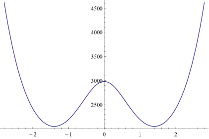
Figure 2: The graphical representation of the function $t\mapsto h_{-2,0}(t)=e^{2\,\log^{2}\left[\frac{1}{2}(\sqrt{t^{2}+4}+t)\right]-8\,t\,\frac{\log\left[\frac{1}{2}(\sqrt{t^{2}+4}+t)\right]}{t^{2}+4}+8}$.

For this total deformation we have that the polar decomposition $F=R\cdot U=V\cdot R$ into the right Biot stretch tensor $U=\sqrt{F^{T}F}$ of the deformation and the orthogonal polar factor $R$ is given by

$$U=\frac{1}{\sqrt{t^{2}+4}}\left(\begin{array}[]{cc}2&t\\ t&t^{2}+2\end{array}\right),\qquad R=\frac{1}{\sqrt{t^{2}+4}}\left(\begin{array}[]{cc}2&t\\ -t&2\end{array}\right).$$ (3.16)

Let us rewrite the right Biot stretch tensor $U$ in the following form

$$U=\frac{\lambda_{1}}{\lambda_{1}^{2}+1}\,\left(\begin{array}[]{cc}2&\lambda_{1}-\frac{1}{\lambda_{1}}\vspace{1.2mm}\\ \lambda_{1}-\frac{1}{\lambda_{1}}&\lambda^{2}+\frac{1}{\lambda_{1}^{2}}\\ \end{array}\right),$$ (3.19)

where $\lambda_{1}=\frac{1}{2}(\sqrt{t^{2}+4}+t)$ denotes the first eigenvalue of $U$. Further, $U$ can be orthogonally diagonalized to

$$U=Q\cdot\left(\begin{array}[]{cc}\frac{1}{\lambda_{1}}&0\\ 0&\lambda_{1}\end{array}\right)\cdot{Q^{T}},$$ (3.22)

where

$$Q=\frac{\sqrt{\lambda_{1}}}{\sqrt{\lambda_{1}^{2}+1}}\,\left(\begin{array}[]{cc}-\sqrt{\lambda_{1}}&\frac{1}{\sqrt{\lambda_{1}}}\vspace{1.2mm}\\ \frac{1}{\sqrt{\lambda_{1}}}&\sqrt{\lambda_{1}}\\ \end{array}\right).$$ (3.25)

Hence, the principal logarithm of $U$ is

$$\log U=Q\cdot\left(\begin{array}[]{cc}-\log\lambda_{1}&0\\ 0&\log\lambda_{1}\end{array}\right)\cdot Q^{T}=\frac{1}{\sqrt{t^{2}+4}}\cdot\left(\begin{array}[]{cc}-t\,\log\lambda_{1}&2\,\log\lambda_{1}\\ 2\,\log\lambda_{1}&t\,\log\lambda_{1}\end{array}\right).$$ (3.30)

We still need to determine a suitable plastic stretch $U_{p}\in{\rm SL}(2)$. The general form of a matrix $U_{p}\in{\rm PSym}(2)$ such that $\textrm{tr}(\log U_{p})=0$ is

$$\log U_{p}=\left(\begin{array}[]{ccc}a&b\\ b&-a\end{array}\right)\quad\Rightarrow\quad U_{p}=\exp\left(\begin{array}[]{ccc}a&b\\ b&-a\end{array}\right).$$ (3.35)

We obtain that

$$\|\operatorname{dev}_{2}\log U-\operatorname{dev}_{2}\log U_{p}\|^{2} =\|\operatorname{dev}_{2}\log U\|^{2}-2\,\langle\operatorname{dev}_{2}\log U,\operatorname{dev}_{2}\log U_{p}\rangle+\|\operatorname{dev}_{2}\log U_{p}\|^{2}$$ (3.36)

$$=2\,\log^{2}\lambda_{1}-2\,\frac{\log\lambda_{1}}{t^{2}+4}(-2\,a\,t+4\,b)+2\,a^{2}+2\,b^{2}.$$

With this representation we are able to disprove rank-one convexity of the function $F\mapsto e^{\|\operatorname{dev}_{2}\log U-\operatorname{dev}_{2}\log U_{p}\|^{2}}$. We have to check the convexity of the function

$$h_{a,b}(t)=W({\boldsymbol{\mathbbm{1}}}+t(\eta\otimes\xi))=e^{2\,\log^{2}\left[\frac{1}{2}(\sqrt{t^{2}+4}+t)\right]-2\,\frac{\log\left[\frac{1}{2}(\sqrt{t^{2}+4}+t)\right]}{t^{2}+4}(-2\,a\,t+4\,b)+2\,a^{2}+2\,b^{2}},\qquad t\in\mathbb{R}.$$

For our purpose, it is enough to find a matrix $U_{p}$, i.e. some values for $a,b\in\mathbb{R}$, such that the function $t\mapsto h_{a,b}(t)$ is not convex. For simplicity, let us choose $b=0$. We remark from Figure 2 that for $b=0$ and $a=-2$, i.e. for $U_{p}=\left(\begin{array}[]{ccc}e^{-2}&0\\ 0&e^{2}\end{array}\right)\in{\rm SL}(2)$, the function

$$t\mapsto h_{-2,0}(t)=e^{2\,\log^{2}\left[\frac{1}{2}(\sqrt{t^{2}+4}+t)\right]-8\,t\,\frac{\log\left[\frac{1}{2}(\sqrt{t^{2}+4}+t)\right]}{t^{2}+4}+8},\qquad t\in\mathbb{R}.$$

is not convex. In the following we prove this observation analytically.

Let us suppose that the function $h_{-2,0}$ is convex. On one hand, this assumption implies that the first derivative $t\mapsto h_{-2,0}^{\prime}(t)$ is a monotone increasing function on $[0,\infty)$ and we would have

$$h_{-2,0}^{\prime}(t)\geq h_{-2,0}^{\prime}(0)\qquad\forall t>0.$$ (3.37)

On the other hand, since $h_{-2,0}(t)=h_{-2,0}(-t)\,\,\forall\,t\in\mathbb{R}$, we deduce that $h_{-2,0}^{\prime}(t)=-h_{-2,0}^{\prime}(-t)\ \text{for all}\ t\in\mathbb{R},$ which implies that $h_{-2,0}^{\prime}(0)=0.$ Hence, we have obtained that

$$h_{-2,0}^{\prime}(t)\geq 0\qquad\forall t>0,$$ (3.38)

which means that $h_{-2,0}$ is a monotone increasing function on $[0,\infty)$. However, this is not true, since

$$h_{-2,0}(0)=e^{8}\approx 2980.96\qquad\text{and}\qquad h_{-2,0}(1)\approx 2193.36.$$ (3.39)

Therefore, the assumption that the function $h_{-2,0}$ is convex leads to a contradiction.

In conclusion, the function $h_{-2,0}$ is not convex, which implies that for $U_{p}$ chosen as above the energy $F\mapsto e^{\|\operatorname{dev}_{2}\log U-\operatorname{dev}_{2}\log U_{p}\|^{2}}$ is not rank-one convex, while $F\mapsto e^{\|\operatorname{dev}_{2}\log U\|^{2}}$ is rank-one convex [58]. This final remark completes the proof. ∎

4 Final remarks

We have shown that the multiplicative plasticity models preserve ellipticity in purely elastic processes at frozen plastic variable provided that the initial elastic response is elliptic, see [57]. Preservation of Legendre-Hadamard ellipticity is, in our view, a property which should be satisfied by any hyperelastic-plastic model since the elastically unloaded material specimen should respond reasonably under further purely elastic loading. However, the much used additive logarithmic model does not preserve Legendre-Hadamard ellipticity in general. In Figure 1 we summarize some properties of the additive logarithmic model and the multiplicative decomposition and we compare it with the small strain plasticity model. In contrast, the formulation based on $e^{\|\operatorname{dev}_{2}\log C_{e}\|^{2}}$ and the multiplicative decomposition remains always rank-one convex. Moreover, the change of a given FEM-implementation of $W_{{}_{\rm H}}$ into $W_{{}_{\rm eH}}$ is nearly free of costs [80, 38, 47, 26]. For more constitutive issues regarding the interesting properties of $W_{{}_{\rm eH}}$ we refer to [58, 45].

References

- [1] F. Armero and. J.C. Simo. A priori stability estimates and unconditionally stable product formula algorithms for nonlinear coupled thermoplasticity. Int. J. Plast., 9(6):749–782, 1993.
- [2] D. Balzani, J. Schröder, D. Gross, and P. Neff. Modeling of Anisotropic Damage in Arterial Walls Based on Polyconvex Stored Energy Functions. In D.R.J. Owen, E. Onate, and B. Suarez, editors, Computational Plasticity VIII, Fundamentals and Applications, Part 2, pages 802–805. CIMNE, Barcelona, 2005.
- [3] A. Bertram. An alternative approach to finite plasticity based on material isomorphisms. Int. J. Plast., 15(3):353–374, 1999.
- [4] O.T. Bruhns, H. Xiao, and A. Mayers. Constitutive inequalities for an isotropic elastic strain energy function based on Hencky’s logarithmic strain tensor. Proc. Roy. Soc. London A, 457:2207–2226, 2001.
- [5] O.T. Bruhns, H. Xiao, and A. Mayers. Finite bending of a rectangular block of an elastic Hencky material. J. Elasticity, 66(3):237–256, 2002.
- [6] O.T. Bruhns, H. Xiao, and A. Meyers. Self-consistent Eulerian rate type elasto-plasticity models based upon the logarithmic stress rate. Int. J. Plast., 15(5):479–520, 1999.
- [7] M.A. Caminero, F.J. Montáns, and K.J. Bathe. Modeling large strain anisotropic elasto-plasticity with logarithmic strain and stress measures. Comp. Struct., 89(11):826–843, 2011.
- [8] C. Carstensen, K. Hackl, and A. Mielke. Non–convex potentials and microstructures in finite–strain plasticity. Proc. Royal Soc. London. Series A: Math. Phys. Eng. Sci., 458:299–317, 2002.
- [9] J. Casey. On elastic-thermo-plastic materials at finite deformations. Int. J. Plasticity, 14(1):173–191, 1998.
- [10] J. Casey and P.M. Naghdi. A remark on the use of the decomposition in plasticity. J. Appl. Mech., 47(3):672–675, 1980.
- [11] J. Casey and P.M. Naghdi. Further constitutive results in finite plasticity. Q J Mechanics Appl Math, 37(2):231–259, 1984.
- [12] S. Cleja-Ţigoiu. Consequences of the dissipative restrictions in finite anisotropic elasto-plasticity. Int. J. Plast., 19(11):1917–1964, 2003.
- [13] S. Cleja-Ţigoiu and L. Iancu. Orientational anisotropy and strength-differential effect in orthotropic elasto-plastic materials. Int. J. Plast., 47:80–110, 2013.
- [14] S. Cleja-Ţigoiu and G.A. Maugin. Eshelby’s stress tensors in finite elastoplasticity. Acta Mech., 139(1-4):231–249, 2000.
- [15] W. Dettmer and S. Reese. On the theoretical and numerical modelling of Armstrong-Frederick kinematic hardening in the finite strain regime. Comp. Meth. Appl. Mech. Eng., 193(1):87–116, 2004.
- [16] E.N. Dvorkin, D. Pantuso, and E.A. Repetto. A finite element formulation for finite strain elasto-plastic analysis based on mixed interpolation of tensorial components. Comp. Meth. Appl. Mech. Eng., 114(1):35–54, 1994.
- [17] F. Ebobisse and P. Neff. Existence and uniqueness for rate-independent infinitesimal gradient plasticity with isotropic hardening and plastic spin. Math. Mech. Solids, 15(6):691–703, 2010.
- [18] M. Eisenberg, C.W. Lee, and A. Phillips. Observations on the theoretical and experimental foundations of thermoplasticity. Int. J. Solids Struct., 13(12):1239–1255, 1977.
- [19] A.L. Eterovic and K.-J. Bathe. A hyperelastic-based large strain elasto-plastic constitutive formulation with combined isotropic-kinematic hardening using the logarithmic stress and strain measures. Int. J. Num. Meth. Eng., 30:1099–1114, 1990.
- [20] G. Gabriel and K.J. Bathe. Some computational issues in large strain elasto-plastic analysis. Comp. and Struct., 56(2):249–267, 1995.
- [21] M.G.D. Geers. Finite strain logarithmic hyperelasto-plasticity with softening: a strongly non-local implicit gradient framework. Comp. Meth. Appl. Mech. Eng., 193(30):3377–3401, 2004.
- [22] I.D. Ghiba, P. Neff, and M. Šilhavý. The exponentiated Hencky-logarithmic strain energy. Improvement of planar polyconvexity. Int. J. Non-Linear Mech., 71:48–51, 2015.
- [23] A.E. Green and P.M. Naghdi. A general theory of an elastic-plastic continuum. Arch. Rat. Mech. Anal., 18:251–281, 1965.
- [24] A.E. Green and P.M. Naghdi. Some remarks on elastic-plastic deformation at finite strain. Int. J. Eng. Sci., 9(12):1219–1229, 1971.
- [25] K. Heiduschke. The logarithmic strain space description. Int. J. Solids Struct., 32(8):1047–1062, 1995.
- [26] K. Heiduschke. Computational aspects of the logarithmic strain space description. Int. J. Solids Struct., 33(5):747–760, 1996.
- [27] D. Henann and L. Anand. A large deformation theory for rate-dependent elastic–plastic materials with combined isotropic and kinematic hardening. Int. J. Plast., 25(10):1833–1878, 2009.
- [28] M. Horák and M. Jirásek. An extension of small-strain models to the large-strain range based on an additive decomposition of a logarithmic strain. In J. Chleboun, K. Segeth, J. Šıstek, and T. Vejchodskỳ, editors, Progr. Algorithms Num. Math., volume 16, pages 88–93. 2013.
- [29] J.W. Hutchinson and K.W. Neale. Finite strain -deformation theory. In D.E. Carlson and R.T. Shield, editors, Proceedings of the IUTAM Symposium on Finite Elasticity, pages 237–247. Martinus Nijhoff, 1982, https://www.uni-due.de/imperia/md/content/mathematik/ag_neff/hutchinson_ellipticity80.pdf.
- [30] M. Itskov. On the application of the additive decomposition of generalized strain measures in large strain plasticity. Mech. Res. Commun., 31(5):507–517, 2004.
- [31] J. Krishnan and D.J. Steigmann. A polyconvex formulation of isotropic elastoplasticity theory. IMA J. Appl. Math., 79:722–738, 2014.
- [32] E.H. Lee. Elastic-plastic deformation at finite strains. J. Appl. Mech., 36(1):1–6, 1969.
- [33] J.D. Lee and Y. Chen. A theory of thermo-visco-elastic-plastic materials: thermomechanical coupling in simple shear. Theoretical Appl. Fract. Mech., 35(3):187–209, 2001.
- [34] J. Löblein, J. Schröder, and F. Gruttmann. Application of generalized measures to an orthotropic finite elasto-plasticity model. Comp. Mat. Sci., 28(3):696–703, 2003.
- [35] J. Lu and P. Papadopoulos. A covariant formulation of anisotropic finite plasticity: theoretical developments. Comp. Meth. Appl. Mech. Eng., 193(48):5339–5358, 2004.
- [36] J. Lubliner. Plasticity theory. Courier Dover Publications, 2008.
- [37] R. Martin and P. Neff. Minimal geodesics on for left-invariant, right--invariant Riemannian metrics. Preprint arXiv: 1409.7849, submited, 2014.
- [38] A. Masud, M. Panahandeh, and F. Aurrichio. A finite-strain finite element model for the pseudoelastic behavior of shape memory alloys. Comp. Meth. Appl. Mech. Eng., 148(1):23–37, 1997.
- [39] G. Maugin. Eshelby stress in elastoplasticity and ductile fracture. Int. J. Plast., 10(4):393–408, 1994.
- [40] C. Miehe, N. Apel, and M. Lambrecht. Anisotropic additive plasticity in the logarithmic strain space: modular kinematic formulation and implementation based on incremental minimization principles for standard materials. Comp. Meth. Appl. Mech. Eng., 191(47):5383–5425, 2002.
- [41] C. Miehe, J. Méndez Diez, S. Göktepe, and L.M. Schänzel. Coupled thermoviscoplasticity of glassy polymers in the logarithmic strain space based on the free volume theory. Int. J. Solids Struct., 48(13):1799–1817, 2011.
- [42] C. Miehe, S. Göktepe, and J. Méndez Diez. Finite viscoplasticity of amorphous glassy polymers in the logarithmic strain space. Int. J. Solids Struct., 46:181–202, 2009.
- [43] A. Mielke. Finite elastoplasticity Lie groups and geodesics on . In P. Newton, P. Holmes, and A. Weinstein, editors, Geometry, Mechanics, and Dynamics, pages 61–90. Springer, 2002.
- [44] A. Mielke. Energetic formulation of multiplicative elasto-plasticity using dissipation distances. Cont. Mech. Thermodyn., 15(4):351–382, 2003.
- [45] G. Montella, S. Govindjee, and P. Neff. The exponentiated Hencky strain energy in modelling tire derived material for moderately large deformations. Preprint arXiv:1509.06541, 2015.
- [46] J. Mosler and M. Ortiz. Variational h-adaption in finite deformation elasticity and plasticity. Int. J. Num. Meth. Eng., 72(5):505–523, 2007.
- [47] R. Naghdabadi, M. Baghani, and J. Arghavani. A viscoelastic constitutive model for compressible polymers based on logarithmic strain and its finite element implementation. Finite Elem. Anal. Des., 62:18–27, 2012.
- [48] P. Neff. Mathematische Analyse multiplikativer Viskoplastizität. Ph.D. thesis, Technische Universität Darmstadt. Shaker Verlag, ISBN:3-8265-7560-1,https://www.uni-due.de/hm0014/Download_files/cism_convexity08.pdf, Aachen, 2000.
- [49] P. Neff. On Korn’s first inequality with nonconstant coefficients. Proc. Roy. Soc. Edinb. A, 132:221–243, 2002.
- [50] P. Neff. Finite multiplicative plasticity for small elastic strains with linear balance equations and grain boundary relaxation. Cont. Mech. Thermodynamics, 15(2):161–195, 2003.
- [51] P. Neff. Some results concerning the mathematical treatment of finite plasticity. In Deformation and Failure in Metallic Materials, pages 251–274. Springer, 2003.
- [52] P. Neff. Remarks on invariant modelling in finite strain gradient plasticity. Technische Mechanik, 28(1):13–21, 2008.
- [53] P. Neff, K. Chełmiński, and H.D. Alber. Notes on strain gradient plasticity: finite strain covariant modelling and global existence in the infinitesimal rate-independent case. Math. Mod. Meth. Appl. Sci., 19:307–346, 2009.
- [54] P. Neff, B. Eidel, and R.J. Martin. Geometry of logarithmic strain measures in solid mechanics. Preprint arXiv:1505.02203, submitted, 2015.
- [55] P. Neff, B. Eidel, F. Osterbrink, and R. Martin. The Hencky strain energy measures the geodesic distance of the deformation gradient to in the canonical left-invariant Riemannian metric on . PAMM, 13(1):369–370, 2013.
- [56] P. Neff and I.D. Ghiba. Comparison of isotropic elasto-plastic models for the plastic metric tensor . In K. Weinberg and A. Pandolfi, editors, Innovative numerical approaches for coupled multi-scale problems, Proc. IUTAM Symposium on innovative numerical approaches for materials and structures in multi-field and multi-scale problems, Burg Schnellenberg, in press, arXiv:1410.2818, Lecture Notes in Applied and Computational Mechanics. Springer, 2015.
- [57] P. Neff and I.D. Ghiba. The exponentiated Hencky-logarithmic strain energy. Part III: Coupling with idealized isotropic finite strain plasticity. to appear in Cont. Mech. Thermod., arXiv:1409.7555, the special issue in honour of D.J. Steigmann, 2015.
- [58] P. Neff, I.D. Ghiba, and J. Lankeit. The exponentiated Hencky-logarithmic strain energy. Part I: Constitutive issues and rank–one convexity. J. Elasticity, doi: 10.1007/s10659-015-9524-7, arXiv:1403.3843, 2015.
- [59] P. Neff, I.D. Ghiba, J. Lankeit, R. Martin, and D.J. Steigmann. The exponentiated Hencky-logarithmic strain energy. Part II: Coercivity, planar polyconvexity and existence of minimizers. Z. Angew. Math. Phys., 66:1671–1693, 2015.
- [60] P. Neff, Y. Nakatsukasa, and A. Fischle. A logarithmic minimization property of the unitary polar factor in the spectral norm and the Frobenius matrix norm. SIAM J. Matrix Analysis, 35:1132–1154, 2014.
- [61] P. Neff, A. Sydow, and C. Wieners. Numerical approximation of incremental infinitesimal gradient plasticity. Int. J. Num. Meth. Eng., 77(3):414–436, 2009.
- [62] P. Neff and C. Wieners. Comparison of models for finite plasticity. A numerical study. Comput. Visual. Sci., 6:23–35, 2003.
- [63] P. Papadopoulos and J. Lu. A general framework for the numerical solution of problems in finite elasto-plasticity. Comp. Meth. Appl. Mech. Eng., 159(1):1–18, 1998.
- [64] P. Papadopoulos and J. Lu. On the formulation and numerical solution of problems in anisotropic finite plasticity. Comp. Meth. Appl. Mech. Eng., 190(37):4889–4910, 2001.
- [65] D. Perić and E.A. de Souza Neto. A new computational model for Tresca plasticity at finite strains with an optimal parametrization in the principal space. Comp. Meth. Appl. Mech. Eng., 171(3):463–489, 1999.
- [66] D. Perić, D.R.J. Owen, and M.E. Honnor. A model for finite strain elasto-plasticity based on logarithmic strains: Computational issues. Comp. Meth. Appl. Mech. Eng., 94(1):35–61, 1992.
- [67] A. Raoult. Non-polyconvexity of the stored energy function of a St.Venant-Kirchhoff material. Aplikace Matematiky, 6:417–419, 1986.
- [68] S. Reese and D. Christ. Finite deformation pseudo-elasticity of shape memory alloys–Constitutive modelling and finite element implementation. Int. J. Plast., 24(3):455–482, 2008.
- [69] S. Reese and P. Wriggers. A material model for rubber-like polymers exhibiting plastic deformation: computational aspects and a comparison with experimental results. Comp. Meth. Appl. Mech. Engrg., 148:279–298, 1997.
- [70] C. Sansour. On the dual variable of the logarithmic strain tensor, the dual variable of the Cauchy stress tensor, and related issues. Int. J. Solids Struct., 38(50):9221–9232, 2001.
- [71] C. Sansour and W. Wagner. Viscoplasticity based on additive decomposition of logarithmic strain and unified constitutive equations: Theoretical and computational considerations with reference to shell applications. Comp. Struct., 81(15):1583–1594, 2003.
- [72] I. Schmidt. Some comments on formulations of anisotropic plasticity. Comp. Mat. Sci., 32(3):518–523, 2005.
- [73] J. Schröder, F. Gruttmann, and J. Löblein. A simple orthotropic finite elasto–plasticity model based on generalized stress–strain measures. Comp. Mech., 30(1):48–64, 2002.
- [74] A.V. Shutov and J. Ihlemann. Analysis of some basic approaches to finite strain elasto-plasticity in view of reference change. Int. J. Plast, 63:183–197, 2014.
- [75] A.V. Shutov and R. Kreißig. Finite strain viscoplasticity with nonlinear kinematic hardening: Phenomenological modeling and time integration. Comp. Meth. Appl. Mech. Eng., 197(21):2015–2029, 2008.
- [76] J.C. Simo. Algorithms for static and dynamic multiplicative plasticity that preserve the classical return mapping schemes of the infinitesimal theory. Comp. Meth. Appl. Mech. Eng., 99(1):61–112, 1992.
- [77] J.C. Simo. Recent developments in the numerical analysis of plasticity. In E. Stein, editor, Progress in computational analysis of inelastic structures, pages 115–173. Springer, 1993.
- [78] J.C. Simo. Numerical analysis and simulation of plasticity. In P.G. Ciarlet and J.L. Lions, editors, Handbook of Numerical Analysis, volume VI. Elsevier, Amsterdam, 1998.
- [79] J.C. Simo and M. Ortiz. A unified approach to finite deformation elastoplastic analysis based on the use of hyperelastic constitutive equations. Comp. Meth. Appl. Mech. Engrg., 49:221–245, 1985.
- [80] E. Tanaka. Finite element investigation of the problem of large strains, formulated in terms of true stress and logarithmic strain. Acta Mech., 34(1-2):129–141, 1979.
- [81] M.H. Ulz. A finite isoclinic elasto-plasticity model with orthotropic yield function and notion of plastic spin. Comp. Meth. Appl. Mech. Eng., 200(21):1822–1832, 2011.
- [82] M.H. Ulz and H. Manfred. A Green–Naghdi approach to finite anisotropic rate-independent and rate-dependent thermo-plasticity in logarithmic Lagrangean strain–entropy space. Comp. Meth. Appl. Mech. Eng., 198(41):3262–3277, 2009.
- [83] H. Xiao, O. Bruhns, and A. Meyers. A consistent finite elastoplasticity theory combining additive and multiplicative decomposition of the stretching and the deformation gradient. Int. J. Plast., 16(2):143–177, 2000.