Moments Preserving and high-resolution Semi-Lagrangian Advection Scheme

Abstract

We present a forward semi-Lagrangian numerical method for systems of transport equations able to advect smooth and discontinuous fields with high-order accuracy. The numerical scheme is composed of an integration of the transport equations along the trajectory of material elements in a moving grid and a reconstruction of the fields in a reference regular mesh using a non-linear mapping and adaptive moment-preserving interpolations. The non-linear mapping allows for the arbitrary deformation of material elements. Additionally, interpolations can represent discontinuous fields using adaptive-order interpolation near jumps detected with a slope-limiter function. Due to the large number of operations during the interpolations, a serial implementation of this scheme is computationally expensive. The scheme has been accelerated in many-core parallel architectures using a thread per grid node and parallel data gathers. We present a series of tests that prove the scheme to be an attractive option for simulating advection equations in multi-dimensions with high accuracy.

1 Introduction

Lagrangian transport schemes refer to the use of the method of characteristics for the integration of partial differential equations with advective derivatives. When used as numerical schemes, the deformation of the discrete fields could lead to the loss of mesh connectivity and non-desirable resolution variability. These problems can be fixed if the method is combined with periodic regularizations or interpolations to a fixed mesh, producing what is known as a semi-Lagrangian scheme [6, 34, 36].

Semi-Lagrangian (SL) transport schemes are among the less restrictive numerical solvers of advection-dominated fluid flow problems, allowing much larger time steps than Eulerian-based advection. They are designed to have the enhanced stability of Lagrangian trajectories and the regular resolution of an Eulerian grid. This is accomplished by using a grid either as the initial or final configuration for every time step, integrating paths either forward or backward in time and using interpolations to reconstruct the fields when needed.

Backward SL schemes are well known in meteorology. They have evolved slowly from 1952 to 1972 [11, 41, 13, 34, 26], and became widely used three decades ago after the work of of Robert [32, 33]. His work was of great importance because the combination of a backward SL scheme with semi-implicit time stepping allowed for one order of magnitude longer time steps than previous schemes, without loosing accuracy and became the basis of many operational models for weather prediction and environmental safety [25, 38, 28]. Since then, many improvements to the method have been presented for the modeling of the atmosphere [see [36] for a review]. The backward SL scheme has been formulated for different number of levels [20, 39], and has been made mass-conservative, for divergence-free flows, using finite-volumes [31, 18, 37, 43, 24], finite-elements [22, 4] and limiters [16], or with special interpolating [3] and non-interpolating procedures [29, 30].

Forward SL schemes have been previously studied in meteorology. Interesting results were produced by Purser and Leslie [17] for a mass-conserving scheme and the globally conservative second and third-order scheme using cascade interpolation presented by Nair et al., [23]. Cascade interpolation is an efficient serial procedure but it is not multi-dimensional nor moment-preserving [27]. Also, there are related forward-trajectory Lagrangian particle methods that represent the fluid as a field of particles that carry a non-deforming basis function with them [12, 21]. In SL methods, nodes are not particles but the vertices of deformable material elements and should take into account variations of the volumes around convergent or divergent points in the flow.

Forward SL schemes have been used successfully in plasma physics to solve the Vlasov equation with phase space particle density functionals [35, 8, 7]. They evolved from a close relative, the particle-in-cell (PIC) scheme [9], that suffered, like any other particle method, from noisy fields. In the PIC scheme, the electric and magnetic fields are computed in a grid, after a deposition or remapping of the particle strengths. The method was improved considering the particle field as a continuum and using interpolations to reconstruct the particle field into the grid after a fix number of time steps, keeping the regular resolution and controlling the noise. The PIC and the SL schemes have been combined in [40], obtaining a forward SL approach that allows reconstructions of the global field after a certain number of time steps, further reducing non-desirable damping effects due to frequent interpolations.

The forward SL scheme studied in this work was first presented for smooth fields in the context of Large-Eddy Simulations (LES) [2]. It has evolved from Vortex-in-cell schemes [5] and the Method of Transport (MoT) [10]. Its main contribution was the introduction of novel high-order moment preserving explicit interpolation formulas named Z-splines which are the collocation basis of finite differences, constructed using Hermite interpolation [1]. This forward SL scheme was applied to reactive flows using the complete three-dimensional compressible Navier-Stokes equations with a reduced combustion model showing almost null numerical diffusion and dispersion.

The main concerns with SL schemes are the low-order iterative backward integration of trajectories, the lack of formal conservation properties, particularly for compressible fields, and the use of computationally expensive high-order interpolations. So far, high-order integration in time has been achieved using forward integrations combined with reconstructions over successive lines or with multi-dimensional maps. Formal conservation has been proved only for incompressible flows using finite-volume flux corrections, Galerkin schemes or high-moments conservative interpolations. While computationally expensive interpolations have remained a fundamental problem until the arrival of the fine-grain parallelism of many-core architectures like the graphics processing units (GPUs).

Here, we have extended the third-order in time forward SL scheme of [2] to allow the advection of discontinuous fields in multi-dimensions, automatically adjusting the interpolation basis around the discontinuity using a slope-limiter criteria. The result is a high-order advection scheme that transports smooth fields without losses in several high-order moments of its distributions while detecting jumps and kinks in the transported fields. Interpolations represent fields near discontinuities with lower order functions to avoid using data across jumps, and suppress spurious oscillations. The algorithm has been parallelized for many-core architectures, using an independent process for each node of the grid. The high-order interpolations are accelerated using the many-core wide memory bandwidth gather operations.

In the next section a detailed description of the numerical scheme is presented. The methods performance and behavior under a variety of tests is shown in the third section. The last section summarizes the work presented in this paper and comments on the applications and further development of the scheme we are currently working on.

2 High-order Forward semi-Lagrangian Transport

We consider the system of $N$ transport equations in one, two or three dimensions, using Einstein’s notation, given by

$$\frac{D}{Dt}{h_{i}}({\bm{x}},t)\equiv\frac{\partial}{\partial t}{h_{i}}+u_{j}\frac{\partial}{\partial x_{j}}{h_{i}}=S_{i}({\bm{h}},{\bm{x}},t),$$ (1)

where $j=1,...,N$ and the velocity vector

$$u_{j}=\frac{dx_{j}}{dt}$$ (2)

defines the equation of motion for a material trajectory $x_{j}=x_{j}\left({\bm{x}}_{0},t\right)$ with initial position $x_{j,0}=x_{j}(t=0)$ and $\frac{D}{Dt}$ is the material derivative.

The integration in time of equations (1) and (2) is possible knowing the velocity field as a function of time, yet being given or as part of the transported quantities $h_{i}$, directly or indirectly.

This is implemented by defining a regular reference regular grid as the initial setup of a deformable Lagrangian grid. The fields evolving on the Lagrangian grid are interpolated back to the reference grid after a certain number of time steps, avoiding highly deformed material elements and reseting the Lagrangian grid and corresponding integration paths. High-order interpolations are needed when reseting the Lagrangian grid to avoid the introduction of errors higher than spatial and temporal discretizations.

The right hand side (RHS) of equation (1) may contain spatial derivatives. This are computed using finite differences on the reference grid. To do so, fields must be interpolated from the Lagrangian to the reference grid. Same interpolations are used to reset the Lagrangian grid to the reference. Time evolution is computed using a low storage, third order Runge–Kutta [42] over a number of time steps before interpolating the required fields on the reference grid. The interpolation strategy is presented in the following section.

2.1 Z-spline interpolations

The interpolation procedure chosen for the construction of a multi-dimensional function from an orthogonal data set, consists of tensor products of an special type of one-dimensional piecewise Hermite polynomials called Z-splines that are the collocation basis of finite differences. To the authors knowledge, this procedure was first introduced in 2003 [1, 2].

The Z-spline $Z_{m}(x)$ interpolating the data $(x_{i},h_{i})$, $i=1,...,n$ with $x_{1}<x_{2}<...<x_{n}$, is a piecewise polynomial function which satisfies the conditions:

$$Z_{m}(x)\in C^{m}([x_{1},x_{n}]),$$ (3)

$$\left.\frac{d^{p}}{dx^{p}}Z_{m}(x)\right|_{x_{j}}=h_{m,j}^{p},\quad\hbox{for}\begin{array}[]{l}p=0,...,m\\ \;j=1,...,n\end{array}$$ (4)

$$\qquad\qquad Z_{m}(x)\in\pi_{2m+1}([x_{i},x_{i+1}])\quad\hbox{for}\;i=1,...,n-1;$$ (5)

where $h_{m,j}^{p}$ is the $p$th order derivative of $h$ obtained by high-order finite differences of $h_{j}$ using the Taylor series from $2m+1$ points as centered as possible, and $\pi_{n}$ stands for the class of polynomials of degree not exceeding $n$, over the field $\mathbb{R}$ of real numbers.

For a regular grid, $x$ is scaled with the grid spacing $\Delta x$ and, without loss of generality, one can assume the grid width to be $1$. Cardinal splines, in general, are special cases of spline interpolations given the data points $x_{j}=j$ for $j\in\mathbb{Z}$. In this situation, the expressions for the Z-splines simplify because all cardinal basis functions have the same form and differ only by integer shifts.

Let $\widetilde{Z}_{m}(x)$ be the basis function for cardinal Z-splines interpolating the data. With this definition the interpolation formula for general data in $\mathbb{R}$ can be written as

$$Z_{m}(x)=\sum_{i=-\infty}^{\infty}h(x_{i})\widetilde{Z}_{m}(x-x_{i}).$$ (6)

The linear, cubic and quintic cardinal Z-splines are given in Appendix A. Important properties of the cardinal Z-splines are:

(a) $\widetilde{Z}_{m}(x)=0$ for $|x|>m+1$, i.e., has compact support.

(b) The first $2m+1$ discrete moments of the cardinal Z-spline basis function $\widetilde{Z}_{m}$ are conserved, i.e., for $n=0,...,m$ we have

$$\sum_{j=-\infty}^{\infty}(x-j)^{n}\widetilde{Z}_{m}(x-j)=\delta_{0n}=\left\{\begin{array}[]{ll}1&$if$\;n=0,\\ 0&$otherwise$.\end{array}\right.$$ (7)

(c) For sufficiently smooth functions, the cardinal Z-spline basis functions are $L_{2}$ accurate to order $2m+1$.

Multi-dimensional Z-spline interpolations in a regular Cartesian mesh are the sum of the products of the neighboring node functional values, with the product of the cardinal Z-splines in every Cartesian direction. Consider a field $h(x,y,z)$ defined on a three dimensional Cartesian space and represented by a set of discrete values $h_{i.j,k}=h(x_{i},y_{j},z_{k})$ on a Cartesian grid. Let $(x,y,z)$ be a point such that $x_{r}<x<x_{r+1}$, $y_{s}<y<y_{s+1}$ and $z_{t}<z<z_{t+1}$ where $r$, $s$ and $t$ are integer indexes that enumerate the points of the Cartesian grid. The interpolation of order $m$ of $h(x,y,z)$ is given by

$$Z_{m}(x,y,z)=\sum_{i=r-m}^{r+m+1}\sum_{j=s-m}^{s+m+1}\sum_{k=t-m}^{t+m+1}h_{i.j,k}\widetilde{Z}_{m}(x-x_{i})\widetilde{Z}_{m}(y-y_{j})\widetilde{Z}_{m}(z-z_{k}).$$ (8)

In a SL scheme the nodes move and therefore is necessary to map them into a regular Cartesian mesh before performing the interpolations. This is discussed in the next subsection.

2.2 Non-linear material element mapping and localization

In this work, high-order interpolations were performed using tensor products of one-dimensional functions in Cartesian grids. General interpolations in non-orthogonal Lagrangian grids are possible using a map to a local Cartesian coordinate system. In the mapped space, the Lagrangian grid is Cartesian in the vicinity of a point of interest in the reference grid, now deformed, where the values of the fields are computed through interpolations based on equation (8).

To perform interpolations at a point on the reference Cartesian grid, the position of the point in the mapped space is required and can be calculated through a Taylor expansion of the mapping function. Furthermore, if the shape of the deformed material elements, represented by the Lagrangian grid, are approximated by Z-splines (8), then Taylor series are finite and nonlinear, and can be inverted to obtain relative positions in the mapped space. Higher order Z-spline representation of the deformed material elements has proven to achieve little improvements compared to using $\widetilde{Z}_{0}(x)$ in the product (8) [2]. All results shown in this paper where obtained using $\widetilde{Z}_{0}(x)$ to approximate the inverse of the mapping function.

Figure 1: A two-dimensional deformed Cartesian grid represented by the dashed lines. A point ${\bm{x}}_{0}^{\prime}$ in the reference Cartesian grid, represented by the continuous lines, inside the shaded material element is shown. The distance to a vertex ${\bm{x}}_{0}$ of the material element, in the mapped space where the material element is transformed into a square, is needed for interpolating fields.

Let ${\bm{x}}^{\prime}$ represent the points of the Cartesian reference grid and ${\bm{x}}$ the points of the Lagrangian grid. Take ${\bm{x}}_{0}^{\prime}$ to be the point where interpolations are required and ${\bm{x}}_{0}$ one of its nearest Lagrangian neighboring points. This means that ${\bm{x}}_{0}^{\prime}$ is enclosed in one of the material elements of which ${\bm{x}}_{0}$ is a vertex, as shown in figure 1 by the shaded deformed element.

Let ${\bm{\xi}}({\bm{x}})$ be the transformation function of the deformed material coordinate system ${\bm{x}}$ to a Cartesian coordinate system in the vicinity of ${\bm{x}}_{0}^{\prime}$. The inverse, ${{\bm{x}}(\bm{\xi}})$, can be approximated using $Z_{0}({\bm{\xi}})$ in (8) and the positions of ${\bm{x}}_{0}$ and the rest of vertices of the Lagrangian element containing ${\bm{x}}_{0}^{\prime}$. In this way, the position of ${\bm{\xi}}_{0}^{\prime}={\bm{\xi}}({\bm{x}}_{0}^{\prime})$ inside the material element in the mapped space can be obtained implicitly through the Taylor expansion

$$\Delta x_{i}=\frac{\partial x_{i}}{\partial\xi_{j}}({\bm{\xi}}_{0})\Delta\xi_{j}+\frac{1}{2}\sum_{j\neq k}\frac{\partial^{2}x_{i}}{\partial\xi_{j}\partial\xi_{k}}({\bm{\xi}}_{0})\Delta\xi_{j}\Delta\xi_{k}$$ (9)

$$+\frac{1}{6}\sum_{j\neq k\neq l}\frac{\partial^{3}x_{i}}{\partial\xi_{j}\partial\xi_{k}\partial\xi_{l}}({\bm{\xi}}_{0})\Delta\xi_{j}\Delta\xi_{k}\Delta\xi_{l},$$

where $\Delta{\bm{x}}={\bm{x}}-{\bm{x}}_{0}^{\prime}$, $\Delta{\bm{\xi}}={\bm{\xi}}-{\bm{\xi}}_{0}^{\prime}$, and the points ${\bm{x}}$ are the vertices of the material element. Finally, as derivatives in equation (9) can be computed, the system can be inverted numerically using Newton’s method to obtain $\Delta{\bm{\xi}}$ and perform interpolations. The initial condition for Newton’s method is obtained by solving (9) ignoring all the non-linear terms.

The possibility of resetting the fields after a number of time steps require the iterative search of a material element. We initialize the search on the opposite direction of the velocity vector and, if the mapping produces coordinates out of the unitary cube, we continue the search on the neighboring cube indicated by the coordinates of the resulted out-of-bounds mapping, repeating the search until the bounded mapping and therefore the material element is found.

2.3 Discontinuities

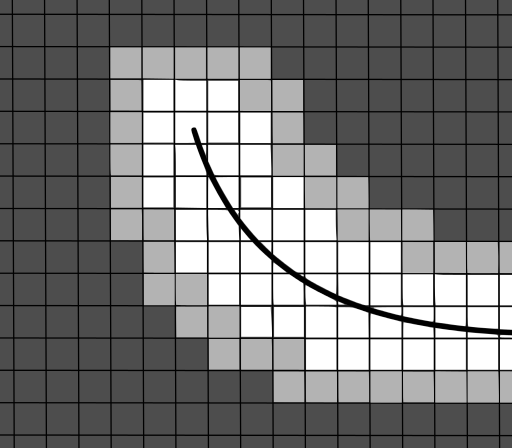
Figure 2: Diagram of the order of the interpolation in the presence of a discontinuity, represented by the curved line, on a Cartesian grid. The dark gray shaded area represents the region where $Z_{2}$ quintic interpolation is used. Light gray is where $Z_{1}$ cubic interpolation is used. Inside white squares, linear interpolation is used.

In order to work with discontinuous distributions and shocks appearing in advection equations, a limiter like jump criterion was introduced. Lets consider a one dimensional discrete distribution $h_{i}=h(x_{i})$ for the sake of simplicity, extension to many dimensions is straight forward. At each time step, a material point $x_{i}$ is marked with a flag whenever the following criterion is met:

$$\frac{|h_{i+1}-2h_{i}+h_{i-1}|}{max\left(|h_{i+1}-h_{i}|,|h_{i}-h_{i-1}|\right)}>0.25.$$ (10)

This represents a comparison of curvatures and slopes that provide a measure of the steepness of the distribution at the material point. In this way, marked points are taken as the approximated location of a the discontinuity.

When interpolations are required, flags are searched among all points needed for the interpolation. If a flag is found, the order of the interpolation is reduced and so the number of points in the vicinity needed for interpolation, to exclude flagged points. The procedure is repeated until linear interpolation is reached or no flagged points can be found in the vicinity required by the interpolation. In this way, as the nodes approach the discontinuity, the interpolation will only use information in one side of the discontinuity. This is represented in figure 2 for the case of the numerical scheme with $Z_{2}$ interpolation. Linear interpolations are used in elements lying at the jump location while cubic interpolations are used when the jump lies a node away.

This procedure naturally introduces numerical dissipation at nodes close to the discontinuities. As the number of nodes flagged near the discontinuity is increasingly localized when spatial resolution is improved, dissipation is considerably reduced with mesh refinement.

3 Results

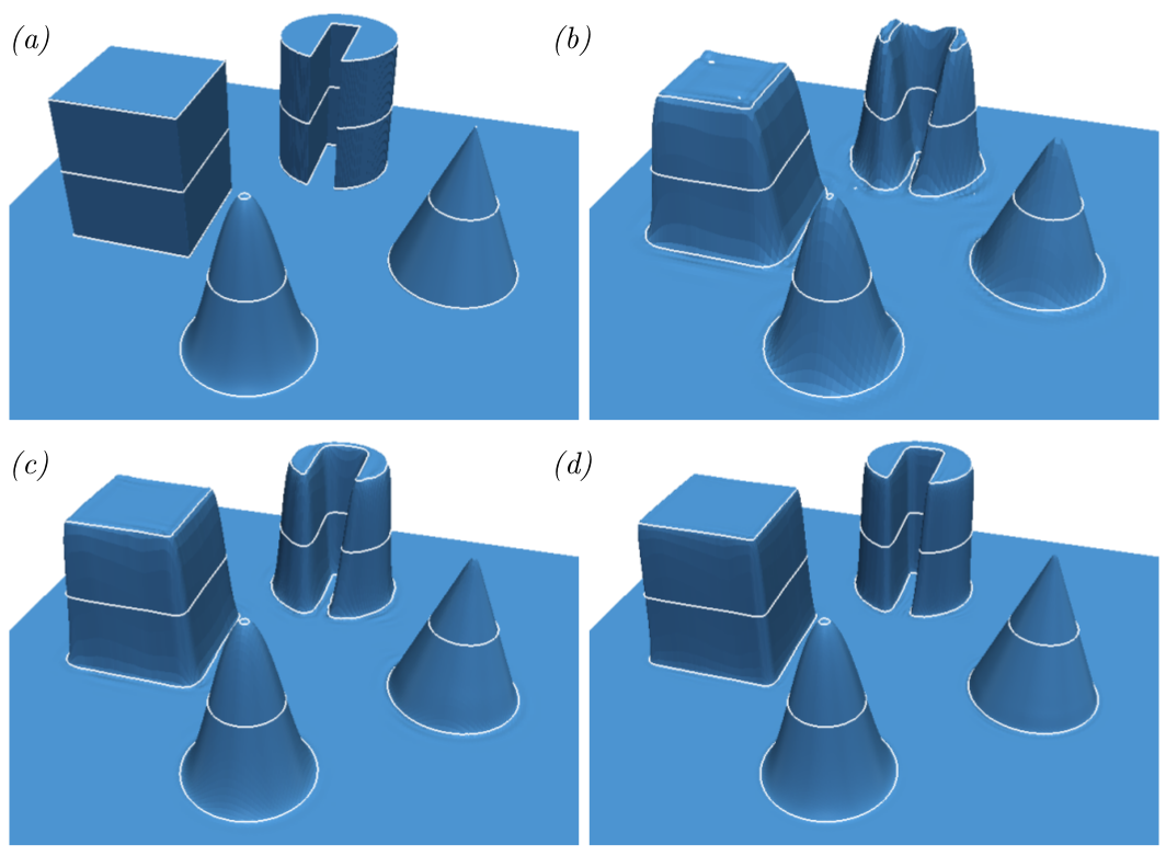
Figure 3: Solid body rotation test after 1 turn. The initial condition is plotted in (a). Solutions after one turn are shown in (b) for a mesh of $128\times 128$ grid points, in (c) for $256\times 256$ and in (d) for $512\times 512$. Contours at values of $h=0.01,0.5,0.99$ are shown.

In this section we present a series of tests that show the method’s performance. First, we solve the pure advection of passive scalar distributions in two dimensions. A cosine hill, a conical and square distributions, and a Zalesak disc are advected by the velocity field of a solid body rotation. Solid body rotation tests are not often shown and reveal numerical diffusion and dispersion produced when computing material derivatives [15, 14, 16]. Pure advection also serves to test the moment preserving properties of the interpolation. Burger’s equation in two dimensions is computed to test advection with shock tracking.

Non-linear shallow water equations are used to compute the dispersion relation of linear waves, the error convergence in the case of Kelvin waves when a Coriolis term is included, and the method’s convergence for nonlinear Kelvin wave dispersion. Kelvin waves are traveling wave solutions for the Coriolis term, in the vicinity of the equator, in the linear limit (small amplitudes). They behave as passive scalar fields in pure advection for small amplitudes, but start shedding equatorial Poincaré waves as amplitude increases. Therefore, they provide a test of the scheme behavior in both limits.

3.1 Pure advection

The advection of a passive, two dimensional scalar distribution $h(x_{1},x_{2})$ by a solid body rotation around the center of the domain $[0,1]\times[0,1]$ given by the velocity field ${\bm{u}}=\Omega(0.5-x_{2},x_{1}-0.5)$ is a solution of the equation

$$\frac{D}{Dt}h=\frac{\partial}{\partial t}h+{\bm{u}}\cdot\nabla h=0,$$ (11)

where $\Omega$ represents the angular velocity of the rotation. The initial condition, shown in figure 3(a), represents a square and a conical distributions along a cosine hill and a Zalesak disc (the notched cylinder), all of unitary height. Figures 3(b), (c) and (d) correspond to surface plots of the solutions for $\Omega=1$ after one turn, for meshes of $128\times 128$, $256\times 256$ and $512\times 512$ grid points respectively.

Contours of values $h=0.01$, $0.5$ and $0.99$ are shown on the surface plots of figure 3. No noticeable distortion of the continuous cosine hill and conical distribution is found after one turn, showing the method computes correctly the advective derivatives of continuous functions for all the spatial resolutions presented.

Contour plots of the solutions for the discontinuous square distribution and Zalesak disc after one turn are in figure 4. Contour values correspond to those of the surface plots ($h=0.01,0.5,0.99$). Interpolation procedures adapt when grid points are in the vicinity of the discontinuities, reducing the order of the interpolation to avoid the use of values across the jumps in their computations. This induces numerical dissipation near the discontinuities, which can bee seen as smoothing of the distributions in figure 3. This is a local effect that depends on the spatial resolution and improves considerably with it, as shown in figure 4. Results show that high resolution is needed when discontinuities appear in the process, but this represent a minor setback because of the efficiency of the method when implemented in massively parallel architectures as the GPU’s.

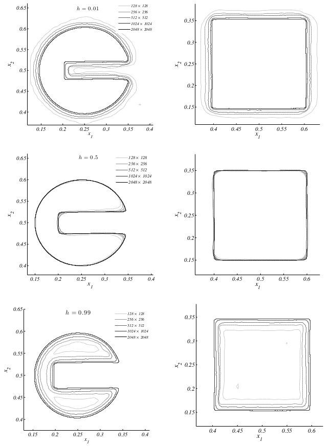
Figure 4: Contour plots for values $h=0.01,0.5,0.99$ for the discontinuous square distribution (right column) and Zalesak disc (left column) after one turn for meshes of $128\times 128$, $256\times 256$, $512\times 512$ and $1024\times 1024$ grid points.

Once the discontinuities are smoothed by the adaptive interpolations, distributions become continuous for a given spatial resolution and the jump criterion ceases to find a discontinuity. This means that no more numerical dissipation is produced as high order interpolations are used everywhere after smoothing. This can bee seen in figure 5 where solutions after two and five turns are shown for different resolutions. Notice that continuous solutions, including the smoothed initially discontinuous, are advected without apparent distortion after five turns.

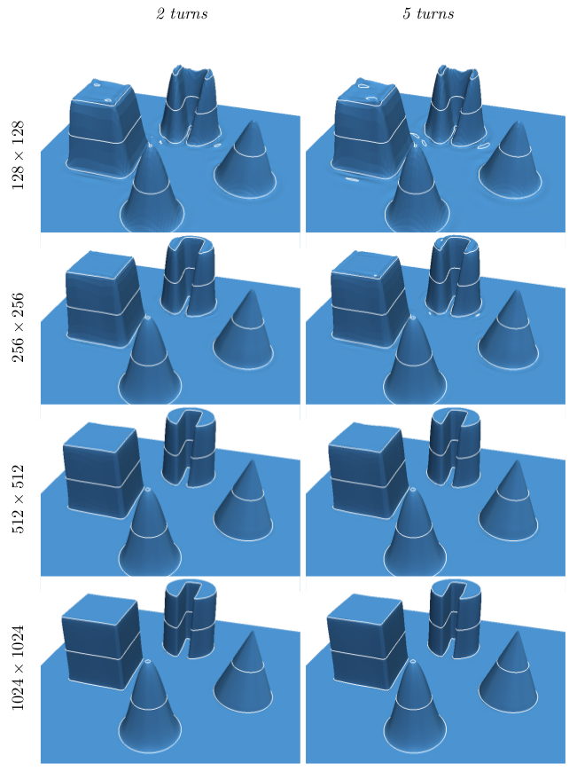
Figure 5: Solid body rotation test after 2 and 5 turns. Subfigures on the left column correspond to solutions after 2 turns, and on the right column are solutions after five turns. Plots corresponding to different number of grids point are organized in rows from $128\times 128$ on top to $1024\times 1024$ at the bottom.

The relative $L_{1}$ error for the continuous cosine hill distribution, given by the initial condition

$$h(x_{1},x_{2})=\left\{\begin{array}[]{@{\hspace{-0.00025in}}l@{\hspace{0.1in}}l@{\hspace{0.1in}}l}0.5\left[1+\cos\left(\frac{\pi\sqrt{\beta}}{0.1}\right)\right]\hfil\hskip 7.22743pt&\hbox{for}\hfil\hskip 7.22743pt&\beta\leq 0.01,\\ 0\hfil\hskip 7.22743pt&\hfil\hskip 7.22743pt&\hbox{otherwise},\end{array}\right.$$ (12)

where $\beta=(x_{1}-0.25)^{2}+(x_{2}-0.5)^{2}$, after one turn are shown in figure 6 for different spatial resolutions. The relative $L_{1}$-error ($\epsilon_{1}$) decays with a slope of $3$ roughly, see figure 6.

The dissipation error is defined as $[\sigma(h)-\sigma(h^{*})]^{2}-[\bar{h}-\bar{h^{*}}]^{2}$ where $\sigma$ is the standard deviation function, $h$ the initial condition 12, $h^{*}$ the numeric solution after one turn, and the over-bar represents the mean value. For a $25\times 25$ mesh, the dissipative error obtained is of approximately $10^{-5}$ with $Z_{2}$ interpolations, two orders of magnitude smaller than what is found with $Z_{1}$ and suitable for all the tests shown in the next section.

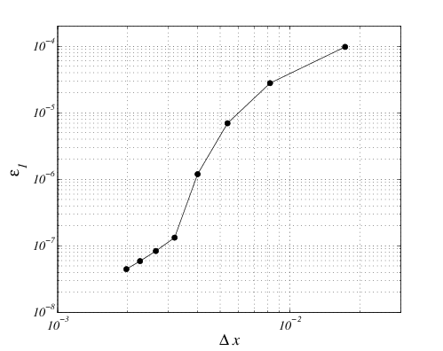
Figure 6: Relative $L_{1}$-error ($\epsilon_{1}$) after one turn for the pure advection of a cosine hill under a solid body rotation velocity field.

Moment preserving properties of the $Z$-spline interpolations are shown in Table 1 for the discrete moments defined as

$$m_{p}=\sum_{i}h_{i}^{*}\left[(x_{1}^{i}-0.5)^{p}+(x_{2}^{i}-0.5)^{p}\right],$$ (13)

where the sum is over all points in the reference grid enumerated by $i$ and $h_{i}^{*}$ is the numerical solution after one turn on the grid point $(x_{1}^{i},x_{2}^{i})$. The table shows $m_{p}$ for $p=0,1,2,3,4$ of the cosine hill distribution using the $Z_{0}$, $Z_{1}$ and $Z_{2}$ interpolations for a $25\times 25$ mesh, and their exact values.

	$m_{0}$	$m_{1}$	$m_{2}$	$m_{3}$	$m_{4}$
Exact	23.3536	-11.6768	6.0558	-3.0820	1.6249
FSL-$Z_{0}$	22.8278	-11.0854	8.0065	-4.1267	3.1567
FSL-$Z_{1}$	23.3553	-11.6787	6.0583	-3.0991	1.6201
FSL-$Z_{2}$	23.3535	-11.6768	6.0559	-3.0822	1.6251

Table 1: Discrete moments of the cosine hill used in the solid body rotation test after one period.

Finally, we comment on the scheme performance when implemented to run in GPU’s. The execution of a time step showed a linear growth from $0.02$ seconds for a $150$ thousand grid points to $0.4$ seconds for a $4$ million grid points on a Nvidia®TeslaK20 Card (CFL number of 0.5). This is characteristic of explicit schemes under fine grain parallelism, when the time evolution of fields on a single node represents a computational thread.

3.2 Burger’s equation

As seen in the previous section, passive discontinuous distributions can be advected by the FSL method using the jump criterion described in Section §2.3 which produced a localized numerical diffusion and a smoothing of the discontinuity as a consequence. Although this gives good results in pure advection, it is not desirable to smooth out discontinuities when solutions should produce shocks. Burger’s equations provides a test to the jump criterion behavior under shock formation. Burger’s equation

$$\frac{D}{Dt}{\bm{u}}=\frac{\partial}{\partial t}{\bm{u}}+{\bm{u}}\cdot\nabla{\bm{u}}={\bm{0}},$$ (14)

is solved in the domain $[0,1]\times[0,1]$ for the initial condition

$${\bm{u}}=\left\{\begin{array}[]{@{\hspace{-0.00025in}}l@{\hspace{0.1in}}l@{\hspace{0.1in}}l}\frac{1}{r}e^{-150(r-0.2)^{2}}(x_{1}-0.5,x_{2}-0.5)\hfil\hskip 7.22743pt&\hbox{for}\hfil\hskip 7.22743pt&r>0.001,\\ {\bm{0}}\hfil\hskip 7.22743pt&\hfil\hskip 7.22743pt&\hbox{otherwise},\end{array}\right.$$ (15)

where $r=\sqrt{(x_{1}-0.5)^{2}+(x_{2}-0.5)^{2}}$.

Shock formation can be seen in figure 7. Solutions show that the jump criterion preserves the shock without apparent diffusion or oscillations in the vicinity of the front. Figure 7(f) suggest convergence to the actual discontinuity as resolution increases.

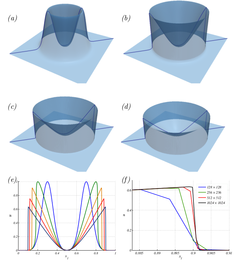
Figure 7: Numerical solution of Burger’s equation in two dimensions. The initial condition is shown in (a). Solutions at times $0.1$, $0.2$ and $0.3$ are shown in (b), (c) and (d) respectively. In (e), a radial slice of solutions at $t=0,0.1,0.2,0.3,0,4$ are compared. A close view of the shock at $t=0.4$ for different grid resolutions can be seen in (f).

Results show that the jump criterion can capture and advect shocks which makes the scheme suitable for a wider variety of applications.

3.3 Non-linear shallow-water equations

The non-linear shallow water equations (NLSW) describe the evolution of the perturbation $h$ of the thickness of a layer of fluid under gravity in the limit were the characteristic wavelength of the perturbation is much larger than the layers thickness. It is the result of vertically averaging the mass and momentum equations of the flow across the layer [19]. The set of equations for $h$ and the horizontal averaged velocity ${\bm{u}}$, the advecting field, can include viscosity effects, topography and Coriolis forces to approximate the behavior of large structures in oceanic and atmospheric flows [19].

NLSW were chosen to test the method in different ways. First, to reproduce the linear dispersion relation of freely oscillating gravity waves, with no viscosity or Coriolis effects. Simulation of Kelvin equatorial waves in the linear regime served to compute the order of the method when the Coriolis term is included in the equations. Convergence of the method for non-linear phenomena was tested computing equatorial Kelvin non-linear wave dispersion.

The non-dimensional shallow-water equations in two spatial dimensions including Coriolis effects and viscosity are given by

$$\frac{D}{Dt}h = -(1+h)\nabla\cdot{\bm{u}},$$

$$\frac{D}{Dt}{\bm{u}} = -\nabla h-f{\bm{u}}^{\bot}+\nu\nabla\cdot\left[(1+h)(\nabla{\bm{u}}+\nabla{\bm{u}}^{T})\right],$$ (16)

where ${\bm{u}}^{\bot}=(-u_{2},u_{1})$ is the orthogonal velocity [19], $f$ is the Coriolis parameter proportional to $x_{2}$ close to the equator, placed in $x_{2}=0$, and $\nu$ is the dimensionless viscosity, taken as a small parameter.

Equations were solved with bi-periodic boundary conditions over a given squared domain $[0,L_{x}]\times[-0.5,0.5]$. For the linear dispersion relations, solutions to (16) where computed for $f=0$, $\nu=0$ and one spatial dimension for a small amplitude sinusoidal perturbation $h$. The plot of the resulting frequency $\omega$ vs the wave number $\kappa$ can be seen in figure 8 for different spatial resolutions. Notice that the computed dispersion relation is correct until a value of $\kappa$ beyond which the spatial discretization fails to represent correctly the sinusoidal wave form.

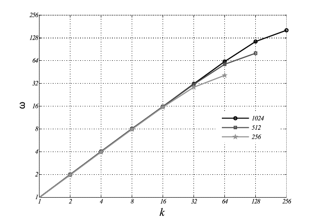
Figure 8: Linear dispersion relation for shallow water waves.

Equatorial NLSW equations without viscosity effects ($\nu=0$, $f=f_{0}x_{2}$) in the small amplitude (linear) limit accept an infinite set of dispersive wave solutions, called Rossby, Yanai and Poincaré waves, and non-dispersive eastward traveling wave solutions called Kelvin waves given by

$$h = e^{-f_{0}x_{2}^{2}/2}K(x_{1}-t),$$

$$u_{1} = e^{-f_{0}x_{2}^{2}/2}K(x_{1}-t),$$

$$u_{2} = 0.$$ (17)

Where $K$ is an arbitrary function of small amplitude [19]. To compute the order of the method we solved NLSW equations (16) for $\nu=0$, $f_{0}=250$ with an initial condition given by (17) with $t=0$ and $K(x_{1})=Ae^{-f_{0}x_{1}^{2}/2}$ with $A=0.0001$. Solutions at dimensionless time $t=1$ were compared with the analytical Kelvin wave solution, the relative $L_{2}$-error ($\epsilon_{2}$) for different space discretization is shown in figure 9. Again, the method shows a third order convergence rate.

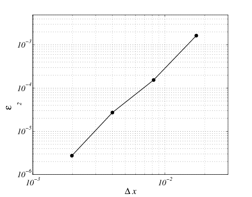
Figure 9: Relative $L_{2}$-error ($\epsilon_{2}$) decay with grid refinement for the equatorial Kelvin wave simulation.

When computing solutions in the nonlinear regime, with initial conditions of larger amplitudes ($A\approx\mathcal{O}(0.1)$), perturbations produce a nonlinear excitation of dispersive Poincaré modes and the formation of a steep front; a known feature of this set of equations [19]. In figure 10 one can see the surface plot of $h$ at time $t=1$ for $\nu=0.0005$, $f_{0}=250$ and the same Gaussian bell initial condition for $h$ and ${\bm{u}}$ previously used, but with a larger amplitude $A=0.5$. Contours drawn on top of the surface $h$ correspond to those plotted for different resolutions showing convergence of the method in the nonlinear regime. Contour values given by $h=-0.001,0.005,0.02,0.1$ and $0.2$ were chosen to reveal the appearance of Poincaré modes characterized by oscillations in both $x_{1}$ and $x_{2}$ directions, which can be noticed in figure 10. Also, contours show convergence of structures of all amplitudes. It most be noticed that a small viscosity is needed to show convergence as nonlinear dispersion of the initial condition will excite infinite Poincaré modes in the inviscid case, from which only a finite set can be represented by a given spatial resolution. This is characteristic of inviscid flow instabilities, and a dissipative mechanism must be included to introduce a minimum scale where flow structures can be represented by the chosen spatial resolution.

Figure 10: Non-linear Kelvin-Poincaré wave dispersion. The surface plot of $h$ at time $t=1$ for an initial Gaussian bell is shown in (a). In (b) contours for the values of $h=-0.001,0.005,0.02,0.1,0.2$, corresponding to those in (a), are plotted for different number of grid points to show convergence. Contours of small scale reveal Poincaré wave structures on the wake.

4 Conclusions

In most fluid phenomena, advection plays an important roll. A numerical scheme capable of making quantitative predictions and simulations must compute correctly the advection terms appearing in the equations governing fluid flow. In many cases, as those where there are viscous effects, numerical errors produced by the computation of material derivatives are diffused away by dissipative mechanisms. Here we present a high order forward semi-Lagrangian numerical scheme specifically tailored to correctly compute material derivatives, as seen by its good performance under advection tests. The success of our scheme relies on the geometrical interpretation of material derivatives to compute the time evolution of fields on grids that deform with the material fluid domain, an interpolating procedure of arbitrary order that preserves the moments of the interpolated distributions, and a nonlinear mapping strategy to perform interpolations between undeformed and deformed grids. Additionally, a discontinuity criterion was implemented to deal with discontinuous fields and shocks. Tests of pure advection, shock formation and nonlinear phenomena are presented to show performance and convergence of the scheme.

On the oder hand, the high computational cost that made impractical this scheme in its origin can now be considerably reduced by massively parallel architectures found in graphic cards. Explicit numerical schemes, like the one presented here, benefit the most from such architectures, they can reduce two to three orders of magnitude the computation times. If we add the fact that graphic processing units give the best operation per monetary cost ratio, our proposed scheme is a very attractive alternative for advective flow simulation.

Extension to three dimensional flows is on its way and the ultimate goal is the development of a code for the full 3D Navier-Stokes equations for both compressible and incompressible phenomena.

Appendix

The $C^{1}$, cubic cardinal Z-spline basis function (equivalent to cubic Bessel interpolation)

$$\widetilde{Z}_{1}(x)=\left\{\begin{array}[]{lll}1-\frac{5}{2}x^{2}+\frac{3}{2}|x|^{3}&$ $&|x|\leq 1,\\ \frac{1}{2}\left(2-|x|\right)^{2}\left(1-|x|\right)&$ $&1\leq|x|\leq 2,\\ 0&$ $&|x|>2.\end{array}\right.$$ (18)

The $C^{2}$, quintic cardinal Z-spline basis function

$$\widetilde{Z}_{2}(x)=\left\{\begin{array}[]{lll}1-\frac{15}{12}x^{2}-\frac{35}{12}|x|^{3}+\frac{63}{12}x^{4}-\frac{25}{12}|x|^{5}&$ $&|x|\leq 1,\\[5.69046pt] -4+\frac{75}{4}|x|-\frac{245}{8}x^{2}\\[2.84544pt] \qquad+\frac{545}{24}|x|^{3}-\frac{63}{8}x^{4}+\frac{25}{24}|x|^{5}&$ $&1\leq|x|\leq 2,\\[5.69046pt] 18-\frac{153}{4}|x|+\frac{255}{8}x^{2}\\[2.84544pt] \qquad-\frac{313}{24}|x|^{3}+\frac{21}{8}x^{4}-\frac{5}{24}|x|^{5}&$ $&2\leq|x|\leq 3,\\[5.69046pt] 0&$ $&|x|>3.\end{array}\right.$$ (19)

Acknowledgments. J. B. S. thanks the support of Professor Rolf Jeltsch. Authors thank Professor Antonmaria Minzoni for his comments and fruitful discussions.

References

- [1] J. T. Becerra-Sagredo. Z-splines: Moment conserving spline interpolation of compact support for arbitrarily spaced data. Technical Report 2003-10, ETH Zürich C. H., 2003.
- [2] J. T. Becerra-Sagredo. High-order semi-Lagrangian numerical method for large-eddy simulations of reacting flows. PhD thesis, ETH Zürich C. H., 2007.
- [3] R. Bermejo. On the equivalence of semi-Lagrangian and particle-in-cell finite-element methods. Mon. Wea. Rev., 118(4):979–987, 1990.
- [4] J. Côté. An accurate and efficient finite-element global model for the shallow-water primitive equations. Mon. Wea. Rev., 118(12):2707–2717, 1990.
- [5] G. H. Cottet and P. D. Koumoutsakos. Vortex methods: theory and practice. Cambridge University Press. U. K., 2000.
- [6] R. Courant, E. Isaacson, and M. Rees. On the solution of nonlinear hyperbolic differential equations by finite differences. Comm. Pure Appl. Math., 52:243–255, 1952.
- [7] N. Crouseilles, M. Mehrenberger, and E. Sonnendrücker. Conservative semi-Lagrangian schemes for Vlasov equations. J. Comp. Phys., 229(6):1927–1953, 2010.
- [8] N. Crouseilles, T. Respaud, and E. Sonnendrücker. A forward semi-Lagrangian method for the numerical solution of the Vlasov equation. Comp. Phys. Comm., 180(10):1730–1745, 2009.
- [9] J. W. Eastwood. The stability and accuracy of EPIC algorithms. Comput. Phys. Comm., 44(1-2):73–82, 1987.
- [10] M. Fey. Ein echt mehrdimensionales Verfahren zur Lösung der Eulergleichungen. PhD thesis, ETH Zürich C. H., 1993.
- [11] R. Fjørtoft. On a numerical method of integrating the barotropic vorticity equations. Tellus, 4(3):179–194, 1952.
- [12] R. A. Gingold and J. J. Monaghan. Smoothed particle hydrodynamics: theory and applications to non-spherical stars. Mon. Not. R. Astron. Soc., 181:375–389, 1977.
- [13] T. N. Krishnamurti. Numerical integration of primitive equations by a quasi-Lagrangian advective scheme. J. Appl. Meteor., 1(4):508–521, 1962.
- [14] D. Kuzmin. Explicit and implicit FEM-FCT algorithms with flux linearization. J. Comp. Phys., 228(7):2517–2534, 2009.
- [15] D. Kuzmin and S. Turek. High-resolution FEM-TVD schemes based on a fully multidimensional flux limiter. J. Comp. Phys., 198(1-2):131–158, 2004.
- [16] M. Lentine, J. T. Gretarsson, and R. Fedkiw. An unconditionally stable fully conservative semi-Lagrangian method. J. Comp. Phys., 230(8):2857–2879, 2011.
- [17] L. M. Leslie and R. J. Purser. Three-dimensional mass-conserving semi-Lagrangian schemes employing forward trajectories. Mon. Wea. Rev., 123:2551–2566, 1995.
- [18] S. J. Lin and R. B. Rood. Multidimensional flux-form semi-Lagrangian transport schemes. Mon. Wea. Rev., 124(9):2046–2070, 1996.
- [19] A. J. Majda, R. R. Rosales, E. G. Tabak, and C. V. Turner. Interaction of Large-Scale Equatorial Waves and Dispersion of Kelvin Waves through Topographic Resonances. J. Atmos. Sci., 56(24):4118–4133, 1999.
- [20] A. McDonald. A semi-Lagrangian and semi-implicit two-time-level integration scheme. Mon. Wea. Rev., 114(5):824–830, 1986.
- [21] J. J. Monaghan. Smoothed particle hydrodynamics. Ann. Rev. Astron. Astrophys., 30:543–574, 1992.
- [22] K. W. Morton. Generalised Galerkin methods for hyperbolic problems. Comp. Meth. Appl. Mech. Eng., 52:847–871, 1985.
- [23] R. D. Nair, J. S. Scroggs, and F. H. M. Semazzi. A forward-trajectory global semi-Lagrangian transport scheme. J. Comput. Phys., 190:275–294, 2003.
- [24] T. Nakamura, R. Tanaka, and K. Takizawa. Exactly conservative semi-Lagrangian scheme for multi-dimensional hyperbolic equations with directional splitting technique. J. Comp. Phys., 174(11):171–207, 2001.
- [25] J. Pudykiewicz. Simulation of the Chernobyl dispersion with a 3D hemispheric tracer model. Tellus, 41B:391–412, 1989.
- [26] D. K. Purnell. Solution of the advective equation by upstream interpolation with a cubic spline. Mon. Wea. Rev., 104:42–48, 1976.
- [27] R. J. Purser and L. M. Leslie. An efficient interpolation procedure for high-order three-dimensional semi-Lagrangian models. Mon. Wea. Rev., 119(10):2492–2498, 1991.
- [28] P. Rasch and D. Williamson. The sensitivity of a general-circulation model climate to the moisture transport. J. Geophys. Res., 96(D7):13,123–13,137, 1991.
- [29] H. Ritchie. Eliminating the interpolation associated with the semi-Lagrangian scheme. Mon. Wea. Rev., 114:135–146, 1986.
- [30] H. Ritchie. Application of the semi-Lagrangian method to a spectral model of the shallow-water equations. Mon. Wea. Rev., 116:1587–1598, 1988.
- [31] P. J. Roache. A flux-based modified method of characteristics. Int. J. Num. Meth. Fluids, 15(11):1259–1275, 1992.
- [32] A. Robert. A stable numerical integration scheme for the primitive meteorological equations. Atmos. Ocean., 19:35–46, 1981.
- [33] A. Robert. A semi-Lagrangian semi-implicit numerical integration scheme for the primitive meteorological equations. J. Meteorolog. Soc. Japan., 60:319–325, 1982.
- [34] J. S. Sawyer. A semi-Lagrangian method of solving the vorticity advection equation. Tellus, 15:336–342, 1963.
- [35] E. Sonnendrücker, J. Roche, P. Bertrand, and A. Ghizzo. The semi-Lagrangian method for the numerical resolution of the Vlasov equation. J. Comput. Phys., 149:201–220, 1999.
- [36] A. Staniforth and J. Côté. Semi-Lagrangian integration schemes for atmospheric models - a review. Mon. Wea. Rev., 119:2206–2223, 1991.
- [37] R. Tanaka, T. Nakamura, and T. Yabe. Constructing exactly conservative scheme in a non-conservative form. Comp. Phys. Comm., 126(3):232–243, 2000.
- [38] M. Tanguay, A. Robert, and R. Laprise. A semi-implicit semi-Lagrangian fully compressible regional forecast model. Mon. Wea. Rev., 118:1970–1980, 1990.
- [39] C. Temperton and A. Staniforth. An efficient two-time-level semi-Lagrangian semi-implicit integration scheme. Quart. J. Roy. Meteor. Soc., 113:1025–1039, 1987.
- [40] S. Vadlamani, S. E. Parker, Y. Chen, and C. Kim. The particle-continuum method: an algorithmic unification of particle in cell and continuum methods. Comput. Phys. Comm., 164:209–213, 2004.
- [41] A. Wiin-Nielsen. On the application of trajectory methods in numerical forecasting. Tellus, 11:180–196, 1959.
- [42] J. H. Williamson. Low-storage Runge-Kutta schemes. J. Comp. Phys., 35:48–56, 1980.
- [43] F. Xiao and T. Yabe. Completely conservative and oscillationless semi-Lagrangian schemes for advection transportation. J. Comp. Phys., 170(2):498–522, 2001.