Abstract

For the search for additional Higgs bosons in the Minimal Supersymmetric Standard Model (MSSM) as well as for future precision analyses in the Higgs sector a precise knowledge of their decay properties is mandatory. We evaluate all two-body decay modes of the heavy Higgs bosons into sfermions in the MSSM with complex parameters (cMSSM). The evaluation is based on a full one-loop calculation of all decay channels, also including hard QED and QCD radiation. The dependence of the heavy Higgs bosons on the relevant cMSSM parameters is analyzed numerically. We find sizable contributions to many partial decay widths. They are roughly of ${\cal O}(15\%)$ of the tree-level results, but can go up to $30\%$ or higher. The size of the electroweak one-loop corrections can be as large as the QCD corrections. The full one-loop contributions are important for the correct interpretation of heavy Higgs boson search results at the LHC and, if kinematically allowed, at a future linear $e^{+}e^{-}$ collider. The evaluation of the branching ratios of the heavy Higgs bosons will be implemented into the Fortran code FeynHiggs.

1 Introduction

One of the most important tasks at the LHC is to search for physics effects beyond the Standard Model (SM), where the Minimal Supersymmetric Standard Model (MSSM) [1, 2, 3] is one of the leading candidates. Supersymmetry (SUSY) predicts two scalar partners for all SM fermions as well as fermionic partners to all SM bosons. Another important task is investigating the mechanism of electroweak symmetry breaking. The most frequently investigated models are the Higgs mechanism within the SM and within the MSSM. Contrary to the case of the SM, in the MSSM two Higgs doublets are required. This results in five physical Higgs bosons instead of the single Higgs boson in the SM; three neutral Higgs bosons, $h_{n}$ ($n=1,2,3$), and two charged Higgs bosons, $H^{\pm}$. The Higgs sector is described at the tree-level by two parameters: the mass of the charged Higgs boson, $M_{H^{\pm}}$, and the ratio of the two vacuum expectation values, $\tan\beta\equiv t_{\beta}=v_{2}/v_{1}$. Often the lightest Higgs boson, $h_{1}$ is identified with the particle discovered at the LHC [4, 5] with a mass around $\sim 125\,\,\mathrm{GeV}$. If the mass of the charged Higgs boson is assumed to be larger than $\sim 200\,\,\mathrm{GeV}$ the four additional Higgs bosons are roughly mass degenerate, $M_{H^{\pm}}\approx m_{h_{2}}\approx m_{h_{3}}$ and referred to as the “heavy Higgs bosons”. Discovering one or more of those additional Higgs bosons would be an unambiguous sign of physics beyond the SM and could yield important information about their supersymmetric origin.

If SUSY is realized in nature and the charged Higgs-boson mass is $M_{H^{\pm}}\lesssim 1.5\,\,\mathrm{TeV}$, then the heavy Higgs bosons could be detectable at the LHC (including its high luminosity upgrade, HL-LHC) and/or at a future linear $e^{+}e^{-}$ collider such as the ILC [6, 7, 8] or CLIC [9]. (Results on the combination of LHC and LC results can be found in Ref. [10].) The discovery potential at the HL-LHC goes up to ${\cal O}(1\,\,\mathrm{TeV})$ for large $\tan\beta$ values and somewhat lower at low $\tan\beta$ values. At an $e^{+}e^{-}$ linear collider the heavy Higgs bosons are pair produced, and the reach is limited by the center of mass energy, $M_{H^{\pm}}\lesssim\sqrt{s}/2$, roughly independent of $\tan\beta$. Details about the discovery process(es) depend strongly on the cMSSM parameters (and will not be further discussed in this paper).

In the case of a discovery of additional Higgs bosons a subsequent precision determination of their properties will be crucial determine their nature and the underlying (SUSY) parameters. In order to yield a sufficient accuracy, one-loop corrections to the various Higgs-boson decay modes have to be considered. Decays to SM fermions have been evaluated at the full one-loop level in the cMSSM in Ref. [11], see also Refs. [12] as well as Refs. [14, 13] for higher-order SUSY corrections. Decays to (lighter) Higgs bosons have been evaluated at the full one-loop level in the cMSSM in Ref. [11], see also Ref. [15]. Decays to SM gauge bosons can evaluated to a very high precision using the full SM one-loop result [16] combined with the appropriate effective couplings [17]. The full one-loop corrections in the cMSSM listed here together with resummed SUSY corrections have been implemented into the code FeynHiggs [19, 18, 20, 17, 21]. Corrections at and beyond the one-loop level in the MSSM with real parameters (rMSSM) are implemented into the code Hdecay [22, 23]. Both codes were combined by the LHC Higgs Cross Section Working Group to obtain the most precise evaluation for rMSSM Higgs boson decays to SM particles and decays to lighter Higgs bosons [24].

The heavy MSSM Higgs bosons can also decay to SUSY particles, i.e. to charginos, neutralinos and scalar fermions. In Ref. [25] it was demonstrated that the SUSY particle modes can dominate the decay of the heavy Higgs bosons. In this work we calculate all two-body decay modes of the heavy Higgs bosons to scalar fermions in the cMSSM. More specifically, we calculate the full one-loop corrections to the partial decay widths

$$\Gamma(h_{n}\to{\tilde{f}}_{i}{\tilde{f}}_{j}^{\dagger})\qquad(n=2,3;\,i,j=1,2)\,,$$ (1)

$$\Gamma(H^{+}\to{\tilde{f}}_{i}{\tilde{f}}_{j}^{\prime\dagger})\quad\text{and}\quad\Gamma(H^{-}\to{\tilde{f}}_{i}^{\dagger}{\tilde{f}^{\prime}}_{j})\qquad(i,j=1,2)\,,$$ (2)

where $H^{\pm}$ denotes the charged, $h_{n}$ the mixed neutral Higgs bosons and $\tilde{f}$ $(\tilde{f^{\dagger}})$ denotes the scalar (anti-) fermions. The total decay width is defined as the sum of the partial decay widths (1) or (2), the SM decay channels as described above and the decays to charginos/neutralinos (at the tree-level, supplemented with effective couplings [17]).

The evaluation of the channels Eqs. (1), (2) is based on a full one-loop calculation, i.e. including (S)QCD and electroweak (EW) corrections, as well as soft and hard QCD and QED radiation. For “mixed” decay modes, we evaluate in addition the two “${\cal CP}$-versions” $(i\neq j)$ of Eq. (1) and the two ‘${\cal CP}$-versions” of Eq. (2), which give different results for non-zero complex phases. While our calculation comprises the decay to all sfermionic decay modes of the cMSSM Higgs bosons, in our numerical analysis we will focus on the decay to the third generation sfermions, scalar top and bottom quarks, scalar tau and tau neutrinos.

Higher-order contributions to MSSM Higgs decays to scalar fermions have been evaluated in various analyses over the last decade. However, they were in most cases restricted to few specific channels. In many cases only parts of a one-loop calculation has been performed, and no higher-order corrections in the cMSSM are available so far. More specifically, the available literature comprises the following. First, ${\cal O}(\alpha_{s})$ corrections to partial decay widths of various squark decay channels in the rMSSM were derived: to the decay of a charged Higgs to stops and sbottoms in Ref. [26], of a heavy Higgs boson to third generation squarks in Ref. [27], supplemented later by an effective resummation of the trilinear Higgs-sbottom coupling in Ref. [28]. First full one-loop corrections in the rMSSM were calculated in the decays of the ${\cal CP}$-odd Higgs boson to scalar quarks [29] and to scalar fermions [30]. The full one-loop corrections in the rMSSM to Higgs decays to squarks was published in Ref. [31]. While there results constitute a full one-loop correction (although not for complex parameters), it differs from our calculation in the renormalization of the SUSY particles and parameters. It was shown in Refs. [32, 33, 34] that our renormalization leads to stable results over nearly the full cMSSM parameters space.

The full ${\cal O}(\alpha_{s})$ corrections to Higgs decays to scalar quarks were also evaluated by a different group in Ref. [35], using a renormalization more similar to ours, but also restricting to the case of real parameters. Finally, in Ref. [36] the ${\cal O}(\alpha_{s})$ corrections to Higgs decays to scalar quarks were re-analyzed, where the emphasis was put on the connection of the MSSM squark sector and Higgs sector couplings to $\overline{\mathrm{MS}}$ input parameters. The latter corrections in particular differ from our treatment of the renormalization of the scalar quark sector. They have been included into the code Hdecay.

In this paper we present for the first time a full one-loop calculation for all two-body sfermionic decay channels of the Higgs bosons in the cMSSM (with no generation mixing), taking into account soft and hard QED and QCD radiation. In Sect. 2 we review the renormalization of all relevant sectors of the cMSSM. Details about the calculation can be found in Sect. 3, and the numerical results for all decay channels are presented in Sect. 4 (including comments on comparisons with results from other groups). The conclusions can be found in Sect. 5. The results will be implemented into the Fortran code FeynHiggs [19, 18, 20, 17, 21].

2 The complex MSSM

The channels (1) and (2) are calculated at the one-loop level, including hard QED and QCD radiation. This requires the simultaneous renormalization of several sectors of the cMSSM, including the colored sector with top and bottom quarks and their scalar partners as well as the gluon and the gluino, the Higgs and gauge boson sector with all the Higgs bosons as well as the $Z$ and the $W$ boson and the chargino/neutralino sector. In the following subsections we briefly review these sectors and their renormalization.

2.1 The Higgs- and gauge-boson sector

The Higgs- and gauge-boson sector follow strictly Ref. [37] and references therein (see especially Ref. [17]). This defines in particular the counterterm $\delta\tan\beta\equiv\delta t_{\beta}$, as well as the counterterms for the $Z$ boson mass, $\delta M_{Z}^{2}$, and the sine of the weak mixing angle, $\delta s_{\mathrm{w}}$.

2.2 The chargino/neutralino sector

The chargino/neutralino sector is also described in detail in Ref. [37] and references therein. In this paper we use the so called CCN scheme, i.e. on-shell conditions for two charginos and one neutralino, which we chose to be the lightest one. In the notation of Ref. [37] we used:

$InoScheme = CCN[1] — fixed CCN scheme with on-shell $\tilde{\chi}_{1}^{0}$.

This defines in particular the counterterm $\delta\mu$, where $\mu$ denotes the Higgs mixing parameter.

2.3 The fermion sector

The fermion sector is described in detail in Ref. [37] and references therein. For simplification we use her the $\smash{\overline{\mathrm{DR}}}$ renormalization for all three generations of down-type quarks and leptons, again in the notation of Ref. [37]:

UVMf1[4, _]  = UVDivergentPart   $\smash{\overline{\mathrm{DR}}}$ renormalization for $m_{d}$, $m_{s}$, $m_{b}$

UVMf1[2, _]  = UVDivergentPart   $\smash{\overline{\mathrm{DR}}}$ renormalization for $m_{e}$, $m_{\mu}$, $m_{\tau}$

2.4 The scalar fermion sector

The sfermion sector which we use here differ slightly form the one described in Ref. [37]. For the squark sector we follow Refs. [32, 33] and for the slepton sector we created an additional $\smash{\overline{\mathrm{DR}}}$ type version in full analogy to the squark sector. In the following we list all these formulas we used in this analysis.

In the absence of non-minimal flavor violation, the sfermion mass matrix is given by [2, 3]

$$\mathbf{M}^{2}_{{\tilde{f}}_{tg}}=\begin{pmatrix}\bigl{(}\mathbf{M}^{2}_{L,f_{t}}\bigr{)}_{gg}+m_{f_{tg}}^{2}&m_{f_{tg}}\bigl{(}\mathbf{X}_{f_{t}}\bigr{)}_{gg}^{*}\\ m_{f_{tg}}\bigl{(}\mathbf{X}_{f_{t}}\bigr{)}_{gg}&\bigl{(}\mathbf{M}^{2}_{R,f_{t}}\bigr{)}_{gg}+m_{f_{tg}}^{2}\end{pmatrix}$$ (3)

where

$$\mathbf{M}^{2}_{L,f_{t}} =M_{Z}^{2}(I_{3}^{f_{t}}-Q_{f_{t}}s_{\mathrm{w}}^{2})c_{2\beta}+\begin{cases}\mathbf{M}^{2}_{\tilde{L}}&\text{for left-handed sleptons ($t=1,2$)}\,,\\ \mathbf{M}^{2}_{\tilde{Q}}&\text{for left-handed squarks ($t=3,4$)}\,,\end{cases}$$

$$\mathbf{M}^{2}_{R,f_{t}} =M_{Z}^{2}Q_{f_{t}}s_{\mathrm{w}}^{2}c_{2\beta}+\begin{cases}\mathbf{M}^{2}_{\tilde{E}}&\text{for right-handed sleptons ($t=2$)}\,,\\ \mathbf{M}^{2}_{\tilde{U}}&\text{for right-handed $u$-type squarks ($t=3$)}\,,\\ \mathbf{M}^{2}_{\tilde{D}}&\text{for right-handed $d$-type squarks ($t=4$)}\,,\\ \end{cases}$$

$$\mathbf{X}_{f_{t}} =\mathbf{A}_{f_{t}}-\mu^{*}\begin{cases}1/t_{\beta}&\text{for isospin-up sfermions ($t=3$)}\,,\\ t_{\beta}&\text{for isospin-down sfermions ($t=2,4$)}\,.\end{cases}$$

The soft-SUSY-breaking parameters $\mathbf{M}^{2}_{\tilde{L},\tilde{Q},\tilde{E},\tilde{U},\tilde{D}}$ and $\mathbf{A}_{f}$ are $3\times 3$ matrices in flavor space whose off-diagonal entries are zero in the minimally flavor-violating MSSM. $Q_{f}$ and $I_{3}^{f}$ denote the charge and the weak iso-spin of the corresponding fermion, and $c_{2\beta}\equiv\cos 2\beta$.

The mass matrix is diagonalized by a unitary transformation ${\mathbf{U}}_{\tilde{f}}$,

$$\mathbf{U}_{\!{\tilde{f}}}\,\mathbf{M}^{2}_{\tilde{f}}\,\mathbf{U}_{\!{\tilde{f}}}^{\dagger}=\begin{pmatrix}m_{{\tilde{f}}_{1}}^{2}&0\\ 0&m_{{\tilde{f}}_{2}}^{2}\end{pmatrix},\qquad\mathbf{U}_{\!{\tilde{f}}}=\begin{pmatrix}U^{\tilde{f}}_{11}&U^{\tilde{f}}_{12}\\ U^{\tilde{f}}_{21}&U^{\tilde{f}}_{22}\end{pmatrix}.$$ (4)

We renormalize the up-type squarks ($\mathrm{\tilde{u}}_{\{g=1,2,3\}}=\{\tilde{u},\tilde{c},\tilde{t}\}$) and the sneutrinos (${\tilde{\nu}}_{\{g=1,2,3\}}=\{\tilde{\nu}_{e},\tilde{\nu}_{\mu},\tilde{\nu}_{\tau}\}$) on-shell (OS). For the down-type squarks ($\mathrm{\tilde{d}}_{\{g=1,2,3\}}=\{\tilde{d},\tilde{s},\tilde{b}\}$) and the electron-type sleptons ($\mathrm{\tilde{e}}_{\{g=1,2,3\}}=\{\tilde{e},\tilde{\mu},\tilde{\tau}\}$) we follow the discussion in Sect. 4 (option $\mathcal{O}2$) of Ref. [32] and renormalize them on-shell. They then have to be computed from a mass matrix with shifted $M_{\tilde{L}}^{2},M_{\tilde{Q}}^{2},M_{\tilde{E}}^{2}$ and $M_{\tilde{D}}^{2}$, see below.

We apply the “$m_{b},A_{b}$ $\smash{\overline{\mathrm{DR}}}$” scheme of Refs. [32, 33]. The scheme affecting sfermions $\mathrm{\tilde{e}}_{g}$, $\mathrm{\tilde{d}}_{g}$ is chosen with the variable $SfScheme[$\mathit{t}$, $\mathit{g}$]:

$SfScheme[2, $$\mathit{g} \text{mixed scheme with $m_{\mathrm{\tilde{e}}_{2g}}$ OS, $A_{\mathrm{e}_{g}}$ $\smash{\overline{\mathrm{DR}}}$}\,,$$] = DR[2] (5a)

$SfScheme[4, $$\mathit{g} \text{mixed scheme with $m_{\mathrm{\tilde{d}}_{2g}}$ OS, $A_{\mathrm{d}_{g}}$ $\smash{\overline{\mathrm{DR}}}$}\,.$$] = DR[2] (5b)

In the following, the sfermion index $\mathit{s}$ runs over both values 1, 2. All sfermions are on-shell,

dMSfsq1[1, 1, 1, $$\mathit{g} \equiv{} \delta m_{{\tilde{\nu}}_{1g}}^{2} =\mathop{\widetilde{\mathrm{Re}}}\bigl{(}\Sigma_{{\tilde{\nu}}_{g}}(m_{{\tilde{\nu}}_{1g}}^{2})\bigr{)}_{11}\,,$$] (6a)

dMSfsq1[$$\mathit{s} \mathit{s} \mathit{g} \equiv{} \delta m_{\mathrm{\tilde{e}}_{sg}}^{2} =\mathop{\widetilde{\mathrm{Re}}}\bigl{(}\Sigma_{\mathrm{\tilde{e}}_{g}}(m_{\mathrm{\tilde{e}}_{sg}}^{2})\bigr{)}_{ss}\,,$$, , 2, ] (6b)

dMSfsq1[$$\mathit{s} \mathit{s} \mathit{g} \equiv{} \delta m_{\mathrm{\tilde{u}}_{sg}}^{2} =\mathop{\widetilde{\mathrm{Re}}}\bigl{(}\Sigma_{\mathrm{\tilde{u}}_{g}}(m_{\mathrm{\tilde{u}}_{sg}}^{2})\bigr{)}_{ss}\,,$$, , 3, ] (6c)

dMSfsq1[$$\mathit{s} \mathit{s} \mathit{g} \equiv{} \delta m_{\mathrm{\tilde{d}}_{sg}}^{2} =\mathop{\widetilde{\mathrm{Re}}}\bigl{(}\Sigma_{\mathrm{\tilde{d}}_{g}}(m_{\mathrm{\tilde{d}}_{sg}}^{2})\bigr{)}_{ss}\,.$$, , 4, ] (6d)

The up-type off-diagonal mass-matrix entries receive counterterms [38, 39, 32]

dMSfsq1[1, 2, 3, $$\mathit{g} \equiv{} \delta Y_{\mathrm{u}_{g}} =\frac{1}{2}\mathop{\widetilde{\mathrm{Re}}}\bigl{(}\Sigma_{\mathrm{\tilde{u}}_{g}}(m_{\mathrm{\tilde{u}}_{1g}}^{2})+\Sigma_{\mathrm{\tilde{u}}_{g}}(m_{\mathrm{\tilde{u}}_{2g}}^{2})\bigr{)}_{12}\,,$$] (7a)

dMSfsq1[2, 1, 3, $$\mathit{g} \equiv{} \delta Y_{\mathrm{u}_{g}}^{*} =\frac{1}{2}\mathop{\widetilde{\mathrm{Re}}}\bigl{(}\Sigma_{\mathrm{\tilde{u}}_{g}}(m_{\mathrm{\tilde{u}}_{1g}}^{2})+\Sigma_{\mathrm{\tilde{u}}_{g}}(m_{\mathrm{\tilde{u}}_{2g}}^{2})\bigr{)}_{21}\,.$$] (7b)

For clarity of notation we furthermore define the auxiliary constants

$$\texttt{dMsq12Sf1[2,\,$\mathit{g}$]}\equiv\delta M_{\mathrm{\tilde{e}}_{g},12}^{2} =m_{\mathrm{e}_{g}}(\delta A_{\mathrm{e}_{g}}^{*}-\mu\,\delta t_{\beta}-t_{\beta}\,\delta\mu)+(A_{\mathrm{e}_{g}}^{*}-\mu\,t_{\beta})\,\delta m_{\mathrm{e}_{g}}\,,$$ (8)

$$\texttt{dMsq12Sf1[4,\,$\mathit{g}$]}\equiv\delta M_{\mathrm{\tilde{d}}_{g},12}^{2} =m_{\mathrm{d}_{g}}(\delta A_{\mathrm{d}_{g}}^{*}-\mu\,\delta t_{\beta}-t_{\beta}\,\delta\mu)+(A_{\mathrm{d}_{g}}^{*}-\mu\,t_{\beta})\,\delta m_{\mathrm{d}_{g}}\,.$$ (9)

The electron/down-type off-diagonal mass counterterms are related as

dMSfsq1[1, 2, 2, $$\mathit{g} \equiv\delta Y_{\mathrm{e}_{g}}=\frac{1}{|U^{\mathrm{\tilde{e}}_{g}}_{11}|^{2}-|U^{\mathrm{\tilde{e}}_{g}}_{12}|^{2}}\Bigl{\{}U^{\mathrm{\tilde{e}}_{g}}_{11}U^{\mathrm{\tilde{e}}_{g}*}_{21}\bigl{(}\delta m_{\mathrm{\tilde{e}}_{1g}}^{2}-\delta m_{\mathrm{\tilde{e}}_{2g}}^{2}\bigr{)}+{}$$] (10a)

$$\kern 120.00018ptU^{\mathrm{\tilde{e}}_{g}}_{11}U^{\mathrm{\tilde{e}}_{g}*}_{22}\delta M_{\mathrm{\tilde{e}}_{g},12}^{2}-U^{\mathrm{\tilde{e}}_{g}}_{12}U^{\mathrm{\tilde{e}}_{g}*}_{21}\delta M_{\mathrm{\tilde{e}}_{g},12}^{2*}\Bigr{\}}\,,$$

dMSfsq1[2, 2, 2, $$\mathit{g} =\delta Y_{\mathrm{e}_{g}}^{*}\,,$$] (10b)

dMSfsq1[1, 2, 4, $$\mathit{g} \equiv\delta Y_{\mathrm{d}_{g}}=\frac{1}{|U^{\mathrm{\tilde{d}}_{g}}_{11}|^{2}-|U^{\mathrm{\tilde{d}}_{g}}_{12}|^{2}}\Bigl{\{}U^{\mathrm{\tilde{d}}_{g}}_{11}U^{\mathrm{\tilde{d}}_{g}*}_{21}\bigl{(}\delta m_{\mathrm{\tilde{d}}_{1g}}^{2}-\delta m_{\mathrm{\tilde{d}}_{2g}}^{2}\bigr{)}+{}$$] (10c)

$$\kern 120.00018ptU^{\mathrm{\tilde{d}}_{g}}_{11}U^{\mathrm{\tilde{d}}_{g}*}_{22}\delta M_{\mathrm{\tilde{d}}_{g},12}^{2}-U^{\mathrm{\tilde{d}}_{g}}_{12}U^{\mathrm{\tilde{d}}_{g}*}_{21}\delta M_{\mathrm{\tilde{d}}_{g},12}^{2*}\Bigr{\}}\,,$$

dMSfsq1[2, 1, 4, $$\mathit{g} =\delta Y_{\mathrm{d}_{g}}^{*}\,.$$] (10d)

The trilinear couplings $A_{f_{tg}}\equiv\bigl{(}\mathbf{A}_{f_{t}}\bigr{)}_{gg}$ are renormalized by

dAf1[2, $$\mathit{g} \mathit{g} \equiv\delta A_{\mathrm{e}_{g}} =\biggl{\{}\frac{1}{m_{\mathrm{e}_{g}}}\Bigl{[}\begin{aligned} &U^{\mathrm{\tilde{e}}_{g}}_{11}U^{\mathrm{\tilde{e}}_{g}*}_{12}(\delta m_{\mathrm{\tilde{e}}_{1g}}^{2}-\delta m_{\mathrm{\tilde{e}}_{2g}}^{2})+{}\\ &U^{\mathrm{\tilde{e}}_{g}}_{11}U^{\mathrm{\tilde{e}}_{g}*}_{22}\delta Y_{\mathrm{e}_{g}}^{*}+U^{\mathrm{\tilde{e}}_{g}*}_{12}U^{\mathrm{\tilde{e}}_{g}}_{21}\delta Y_{\mathrm{e}_{g}}-(A_{\mathrm{e}_{g}}-\mu^{*}t_{\beta})\,\delta m_{\mathrm{e}_{g}}\hbox to0.0pt{$\Bigr{]}+{}$\hss}\end{aligned}$$, ] (11a)

$$\qquad\delta\mu^{*}t_{\beta}+\mu^{*}\delta t_{\beta}\biggr{\}}_{\mathrm{div}}\,,$$

dAf1[3, $$\mathit{g} \mathit{g} \equiv\delta A_{\mathrm{u}_{g}} =\frac{1}{m_{\mathrm{u}_{g}}}\Bigl{[}\begin{aligned} &U^{\mathrm{\tilde{u}}_{g}}_{11}U^{\mathrm{\tilde{u}}_{g}*}_{12}(\delta m_{\mathrm{\tilde{u}}_{1g}}^{2}-\delta m_{\mathrm{\tilde{u}}_{2g}}^{2})+{}\\ &U^{\mathrm{\tilde{u}}_{g}}_{11}U^{\mathrm{\tilde{u}}_{g}*}_{22}\delta Y_{\mathrm{u}_{g}}^{*}+U^{\mathrm{\tilde{u}}_{g}*}_{12}U^{\mathrm{\tilde{u}}_{g}}_{21}\delta Y_{\mathrm{u}_{g}}-\bigl{(}A_{\mathrm{u}_{g}}-\mu^{*}/t_{\beta}\bigr{)}\,\delta m_{\mathrm{u}_{g}}\hbox to0.0pt{$\Bigr{]}+{}$\hss}\end{aligned}$$, ] (11b)

$$\qquad\delta\mu^{*}/t_{\beta}-\mu^{*}\delta t_{\beta}/t_{\beta}^{2}\,,$$

dAf1[4, $$\mathit{g} \mathit{g} \equiv\delta A_{\mathrm{d}_{g}} =\biggl{\{}\frac{1}{m_{\mathrm{d}_{g}}}\Bigl{[}\begin{aligned} &U^{\mathrm{\tilde{d}}_{g}}_{11}U^{\mathrm{\tilde{d}}_{g}*}_{12}(\delta m_{\mathrm{\tilde{d}}_{1g}}^{2}-\delta m_{\mathrm{\tilde{d}}_{2g}}^{2})+{}\\ &U^{\mathrm{\tilde{d}}_{g}}_{11}U^{\mathrm{\tilde{d}}_{g}*}_{22}\delta Y_{\mathrm{d}_{g}}^{*}+U^{\mathrm{\tilde{d}}_{g}*}_{12}U^{\mathrm{\tilde{d}}_{g}}_{21}\delta Y_{\mathrm{d}_{g}}-\bigl{(}A_{\mathrm{d}_{g}}-\mu^{*}t_{\beta}\bigr{)}\,\delta m_{\mathrm{d}_{g}}\hbox to0.0pt{$\Bigr{]}+{}$\hss}\end{aligned}$$, ] (11c)

$$\qquad\,\delta\mu^{*}t_{\beta}+\mu^{*}\delta t_{\beta}\biggr{\}}_{\mathrm{div}}\,,$$

where the subscripted “div” means to take the divergent part, to effect $\smash{\overline{\mathrm{DR}}}$ renormalization of $A_{\mathrm{e}_{g}}$ and $A_{\mathrm{d}_{g}}$ [32].

As now all the sfermion masses are renormalized as on-shell an explicit restoration of the $SU(2)$ relation is needed. This is performed in requiring that the left-handed (bare) soft SUSY-breaking mass parameter is the same in the $\mathrm{\tilde{d}}_{g}$ as in the $\mathrm{\tilde{u}}_{g}$ squark sector at the one-loop level (see also Refs. [40, 41, 42]),

$$M_{\tilde{L}}^{2}(\mathrm{\tilde{e}}_{g}) =M_{\tilde{L}}^{2}({\tilde{\nu}}_{g})+\delta M_{\tilde{L}}^{2}({\tilde{\nu}}_{g})-\delta M_{\tilde{L}}^{2}(\mathrm{\tilde{e}}_{g})\,,$$ (12a)

$$M_{\tilde{Q}}^{2}(\mathrm{\tilde{d}}_{g}) =M_{\tilde{Q}}^{2}(\mathrm{\tilde{u}}_{g})+\delta M_{\tilde{Q}}^{2}(\mathrm{\tilde{u}}_{g})-\delta M_{\tilde{Q}}^{2}(\mathrm{\tilde{d}}_{g})$$ (12b)

with

$$\delta M_{\tilde{L},\tilde{Q}}^{2}({\tilde{f}}_{g}) =|U_{11}^{{\tilde{f}}_{g}}|^{2}\delta m_{{\tilde{f}}_{1g}}^{2}+|U_{12}^{{\tilde{f}}_{g}}|^{2}\delta m_{{\tilde{f}}_{2g}}^{2}-U_{22}^{{\tilde{f}}_{g}}U_{12}^{{\tilde{f}}_{g}*}\delta Y_{f_{g}}-U_{12}^{{\tilde{f}}_{g}}U_{22}^{{\tilde{f}}_{g}*}\delta Y_{f_{g}}^{*}-2m_{f_{g}}\delta m_{f_{g}}$$

$$\quad+M_{Z}^{2}\,c_{2\beta}\,Q_{f_{g}},\delta s_{\mathrm{w}}^{2}-(I_{3}^{f_{g}}-Q_{f_{g}}s_{\mathrm{w}}^{2})(c_{2\beta}\,\delta M_{Z}^{2}+M_{Z}^{2}\,\delta c_{2\beta})\,.$$ (13)

Now $M_{\tilde{L}}^{2}(\mathrm{\tilde{e}}_{g})$ and $M_{\tilde{Q}}^{2}(\mathrm{\tilde{d}}_{g})$ are used in the scalar mass matrix instead of the parameters $M_{\tilde{L},\tilde{Q}}^{2}$ in Eq. (3) when calculating the values of $m_{\mathrm{\tilde{e}}_{sg}}$ and $m_{\mathrm{\tilde{d}}_{sg}}$. However, with this procedure, also $m_{\mathrm{\tilde{e}}_{2g}}$ and $m_{\mathrm{\tilde{d}}_{2g}}$ are shifted, which contradicts our choice of independent parameters. To keep this choice, also the right-handed soft SUSY-breaking mass parameters $M_{\tilde{E},\tilde{D}}^{2}$ receive a shift:

$$M_{\tilde{E}}^{2}(\mathrm{\tilde{e}}_{g}) =\frac{m_{\mathrm{e}_{g}}^{2}\,|X_{\mathrm{e}_{g}}|^{2}}{M_{\tilde{L}}^{2}(\mathrm{\tilde{e}}_{g})+m_{\mathrm{e}_{g}}^{2}+c_{2\beta}M_{Z}^{2}(I_{3}^{\mathrm{e}}-Q_{\mathrm{e}}s_{\mathrm{w}}^{2})-m_{\mathrm{\tilde{e}}_{2g}}^{2}}-m_{\mathrm{e}_{g}}^{2}-c_{2\beta}M_{Z}^{2}Q_{\mathrm{e}}s_{\mathrm{w}}^{2}+m_{\mathrm{\tilde{e}}_{2g}}^{2}\,,$$ (14a)

$$M_{\tilde{D}}^{2}(\mathrm{\tilde{d}}_{g}) =\frac{m_{\mathrm{d}_{g}}^{2}\,|X_{\mathrm{d}_{g}}|^{2}}{M_{\tilde{Q}}^{2}(\mathrm{\tilde{d}}_{g})+m_{\mathrm{d}_{g}}^{2}+c_{2\beta}M_{Z}^{2}(I_{3}^{\mathrm{d}}-Q_{\mathrm{d}}s_{\mathrm{w}}^{2})-m_{\mathrm{\tilde{d}}_{2g}}^{2}}-m_{\mathrm{d}_{g}}^{2}-c_{2\beta}M_{Z}^{2}Q_{\mathrm{d}}s_{\mathrm{w}}^{2}+m_{\mathrm{\tilde{d}}_{2g}}^{2}\,.$$ (14b)

Taking into account this shift in $M_{\tilde{E},\tilde{D}}^{2}$, up to one-loop order, the resulting mass parameter $m_{\mathrm{\tilde{e}}_{1g}}$ and $m_{\mathrm{\tilde{d}}_{1g}}$ are the same as the on-shell mass

$$\bigl{(}m_{\mathrm{\tilde{e}}_{sg}}^{\mathrm{OS}}\bigr{)}^{2} =m_{\mathrm{\tilde{e}}_{sg}}^{2}+\delta m_{\mathrm{\tilde{e}}_{sg}}^{2}-\mathop{\widetilde{\mathrm{Re}}}\bigl{(}\Sigma_{\mathrm{\tilde{e}}_{g}}(m_{\mathrm{\tilde{e}}_{sg}}^{2})\bigr{)}_{ss}\,,$$ (15a)

$$\bigl{(}m_{\mathrm{\tilde{d}}_{sg}}^{\mathrm{OS}}\bigr{)}^{2} =m_{\mathrm{\tilde{d}}_{sg}}^{2}+\delta m_{\mathrm{\tilde{d}}_{sg}}^{2}-\mathop{\widetilde{\mathrm{Re}}}\bigl{(}\Sigma_{\mathrm{\tilde{d}}_{g}}(m_{\mathrm{\tilde{d}}_{sg}}^{2})\bigr{)}_{ss}\,.$$ (15b)

The input parameters in the $b/\tilde{b}$ sector have to correspond to the chosen renormalization. We start by defining the bottom mass, where the experimental input is the SM $\overline{\mathrm{MS}}$ mass [45],

$$m_{b}^{\overline{\mathrm{MS}}}(m_{b}) =4.18\,\,\mathrm{GeV}\,.$$ (16)

To convert to the $\smash{\overline{\mathrm{DR}}}$ mass the following procedure is taken. The value of $m_{b}^{\overline{\mathrm{MS}}}(\mu_{R})$ (at the renormalization scale $\mu_{R}$) is calculated from $m_{b}^{\overline{\mathrm{MS}}}(m_{b})$ at the three-loop level

$$m_{b}^{\overline{\mathrm{MS}}}(\mu_{R}) =m_{b}^{\overline{\mathrm{MS}}}(m_{b})\;\frac{c(\alpha_{s}^{\overline{\mathrm{MS}},(n_{f})}(\mu_{R})/\pi)}{c(\alpha_{s}^{\overline{\mathrm{MS}},(n_{f})}(m_{b})/\pi)}$$ (17)

via the function $c(x)$ following the prescription given in Ref. [46]. $n_{f}$ denotes the number of active flavors. The “on-shell” mass is connected to the $\overline{\mathrm{MS}}$ mass via

$$m_{b}^{\mathrm{os}} =m_{b}^{\overline{\mathrm{MS}}}(\mu_{R})\;\left[1+\frac{\alpha_{s}^{\overline{\mathrm{MS}},(n_{f})}(\mu_{R})}{\pi}\left(\frac{4}{3}+2\,\ln\frac{\mu_{R}}{m_{b}^{\overline{\mathrm{MS}}}(\mu_{R})}\right)+\ldots\right]\,,$$ (18)

where the ellipsis denote the two- and three-loop contributions which can also be found in Ref. [46]. The $\smash{\overline{\mathrm{DR}}}$ bottom quark mass at the scale $\mu_{R}$ is calculated iteratively from [47, 39, 44]

$$m_{b}^{\smash{\overline{\mathrm{DR}}}} =m_{b}^{\mathrm{os}}+\frac{\delta m_{b}^{\mathrm{OS}}-\delta m_{b}^{\smash{\overline{\mathrm{DR}}}}}{|1+\Delta_{b}|}$$ (19)

with an accuracy of $|1-(m_{b}^{\smash{\overline{\mathrm{DR}}}})^{(n)}/(m_{b}^{\smash{\overline{\mathrm{DR}}}})^{(n-1)}|<10^{-5}$ reached in the $n$th step of the iteration.

The quantity $\Delta_{b}$ [47, 48, 49] resums the ${\cal O}((\alpha_{s}t_{\beta})^{n})$ and ${\cal O}((\alpha_{t}t_{\beta})^{n})$ terms and is given by

$$\Delta_{b}=-\frac{\mu^{*}\,t_{\beta}}{\pi}\left[\frac{2}{3}\,\alpha_{s}(m_{t})\,M_{3}^{*}\,I(m_{\tilde{b}_{1}}^{2},m_{\tilde{b}_{2}}^{2},m_{\tilde{g}}^{2})\;+\frac{1}{4}\,\alpha_{t}(m_{t})\,A_{t}^{*}\,I(m_{\tilde{t}_{1}}^{2},m_{\tilde{t}_{2}}^{2},|\mu|^{2})\right]$$ (20)

with

$$I(a,b,c)=C_{0}(0,0,0,a,b,c)=-\frac{ab\ln(b/a)+ac\ln(a/c)+bc\ln(c/b)}{(c-a)(c-b)(b-a)}\,.$$ (21)

Here $\alpha_{t}$ is defined in terms of the top Yukawa coupling $y_{t}(m_{t})=\sqrt{2}m_{t}(m_{t})/v$ as $\alpha_{t}(m_{t})=y_{t}^{2}(m_{t})/(4\pi)$ with $v=1/\sqrt{\sqrt{2}\,G_{F}}=246.218\,\,\mathrm{GeV}$ and $m_{t}(m_{t})\approx m_{t}/(1-\frac{1}{2\,\pi}\alpha_{t}(m_{t})+\frac{4}{3\,\pi}\alpha_{s}(m_{t}))$. Setting in the evaluation of $\Delta_{b}$ the scale to $m_{t}$ was shown to yield in general a more stable result [13] as long as two-loop corrections to $\Delta_{b}$ are not included. $M_{3}$ is the soft SUSY-breaking parameter for the gluinos. We have neglected any CKM mixing of the quarks.

The $Z$ factors of the squark fields are derived in the OS scheme. They can be found in Ref. [37].

2.5 The gluon/gluino sector and the strong coupling constant

The gluon and gluino sector follow strictly Ref. [37]; see also the references therein.

The decoupling of the heavy particles and the running is taken into account in the definition of $\alpha_{s}$: starting point is [45]

$$\alpha_{s}^{\overline{\mathrm{MS}},(5)}(M_{Z}) =0.1184\,,$$ (22)

where the running of $\alpha_{s}^{\overline{\mathrm{MS}},(n_{f})}(\mu_{R})$ can be found in Ref. [45]. $\mu_{R}$ denotes the renormalization scale which is typically of the order of the energy scale of the considered process.

From the $\overline{\mathrm{MS}}$ value the $\smash{\overline{\mathrm{DR}}}$ value is obtained at the two-loop level via the phenomenological one-step formula [50]

$$\alpha_{s}^{\smash{\overline{\mathrm{DR}}},(n_{f})}(\mu_{R}) =\alpha_{s}^{\overline{\mathrm{MS}},(n_{f})}(\mu_{R})\,\Bigg{\{}1+\frac{\alpha_{s}^{\overline{\mathrm{MS}},(n_{f})}(\mu_{R})}{\pi}\left(\frac{1}{4}-\zeta^{(n_{f})}_{1}\right)+$$

$$\quad\left(\frac{\alpha_{s}^{\overline{\mathrm{MS}},(n_{f})}(\mu_{R})}{\pi}\right)^{2}\left[\frac{11}{8}-\frac{n_{f}}{12}-\frac{1}{2}\zeta^{(n_{f})}_{1}+2\,(\zeta^{(n_{f})}_{1})^{2}-\zeta^{(n_{f})}_{2}\right]\Bigg{\}}\,,$$ (23)

where (for $n_{f}=6$)

$$\zeta^{(6)}_{1}=-\ln\frac{\mu_{R}^{2}}{\tilde{M}^{2}}\,,\qquad\zeta^{(6)}_{2}=-\frac{65}{32}-\frac{5}{2}\,\ln\frac{\mu_{R}^{2}}{\tilde{M}^{2}}+\left(\ln\frac{\mu_{R}^{2}}{\tilde{M}^{2}}\right)^{2}\,,$$ (24)

with $\tilde{M}^{2}$ being defined as the geometric average of all squark masses multiplied with the gluino mass, $\tilde{M}^{2}=m_{\tilde{g}}\,\prod_{{\tilde{q}}}(m_{{\tilde{q}}_{1}}m_{{\tilde{q}}_{2}})^{\frac{1}{12}}$. The log terms originates from the decoupling of the SQCD particles from the running of $\alpha_{s}$ at lower scales $\mu_{R}\leq\mu_{\text{dec.}}$. For simplification we have chosen the energy scale of the considered processes (as a typical SUSY scale) also as decoupling scale.

3 Calculation of loop diagrams

In this section we give some details about the calculation of the higher-order corrections to the partial decay widths of Higgs bosons. Sample diagrams are shown in Figs. 1 and 2. Not shown are the diagrams for real (hard and soft) photon and gluon radiation. They are obtained from the corresponding tree-level diagrams by attaching a photon (gluon) to the electrically (color) charged particles. The internal generically depicted particles in Figs. 1 and 2 are labeled as follows: $F$ can be a SM fermion $f$, chargino $\tilde{\chi}_{j}^{\pm}$, neutralino $\tilde{\chi}_{k}^{0}$, or gluino ${\tilde{g}}$; $S$ can be a sfermion ${\tilde{f}}_{i}$ or a Higgs boson $h_{n}$; $U$ denotes the ghosts $u_{V}$; $V$ can be a photon $\gamma$, gluon $g$, or a massive SM gauge boson, $Z$ or $W^{\pm}$. For internally appearing Higgs bosons no higher-order corrections to their masses or couplings are taken into account; these corrections would correspond to effects beyond one-loop order. For external Higgs bosons, as described in Sect. 2.1, the appropriate $\hat{Z}$ factors are applied and on-shell masses (including higher-order corrections) are used [17], obtained with FeynHiggs [19, 18, 20, 17, 21].

Figure 1: Generic Feynman diagrams for the decay $h_{n}\to{\tilde{f}}_{i}{\tilde{f}}_{j}$ ($n=2,3;\,i,j=1,2$). $F$ can be a SM fermion, chargino, neutralino, or gluino; $S$ can be a sfermion or a Higgs boson; $U$ denotes the ghosts; $V$ can be a $\gamma$, $Z$, $W^{\pm}$, or $g$. Not shown are the diagrams with a $h_{n}$–$Z$ or $h_{n}$–$G$ transition contribution on the external Higgs boson leg.

Figure 2: Generic Feynman diagrams for the decay $H^{+}\to{\tilde{f}}_{i}{\tilde{f}}_{j}^{\prime}$ ($i,j=1,2$). (It should be noted that all arrows are inverted in case of a $H^{-}$ decay.) $F$ can be a SM fermion, chargino, neutralino, or gluino; $S$ can be a sfermion or a Higgs boson; $U$ denotes the ghosts; $V$ can be a $\gamma$, $Z$, $W^{\pm}$, or $g$. Not shown are the diagrams with a $H^{\pm}$–$W^{\pm}$ or $H^{\pm}$–$G^{\pm}$ transition contribution on the external Higgs boson leg.

Also not shown are the diagrams with a Higgs boson–gauge/Goldstone self-energy contribution on the external Higgs boson leg. They appear in the decay $h_{n}\to{\tilde{f}}_{i}{\tilde{f}}_{j}$, Fig. 1, with a $h_{n}$–$Z/G$ transition and in the decay $H^{\pm}\to{\tilde{f}}_{i}{\tilde{f}^{\prime}}_{j}$, Fig. 2, with a $H^{\pm}$–$W^{\pm}$/$G^{\pm}$ transition.

Furthermore, in general, in Figs. 1 and 2 we have omitted diagrams with self-energy type corrections of external (on-shell) particles. While the contributions from the real parts of the loop functions are taken into account via the renormalization constants defined by on-shell renormalization conditions, the contributions coming from the imaginary part of the loop functions can result in an additional (real) correction if multiplied by complex parameters (such as $A_{f}$). In the analytical and numerical evaluation, these diagrams have been taken into account via the prescription described in Ref. [37].

Within our one-loop calculation we neglect finite width effects that can help to cure threshold singularities. Consequently, in the close vicinity of those thresholds our calculation does not give a reliable result. Switching to a complex mass scheme [51] would be another possibility to cure this problem, but its application is beyond the scope of our paper.

The diagrams and corresponding amplitudes have been obtained with FeynArts [52]. The model file, including the MSSM counterterms, is largely based on Ref. [37], however adjusted to match exactly the renormalization prescription described in Sect. 2. The further evaluation has been performed with FormCalc and LoopTools [53].

Ultraviolet divergences

As regularization scheme for the UV divergences we have used constrained differential renormalization [54], which has been shown to be equivalent to dimensional reduction [55] at the one-loop level [53]. Thus the employed regularization scheme preserves SUSY [56, 57] and guarantees that the SUSY relations are kept intact, e.g. that the gauge couplings of the SM vertices and the Yukawa couplings of the corresponding SUSY vertices also coincide to one-loop order in the SUSY limit. Therefore no additional shifts, which might occur when using a different regularization scheme, arise. All UV divergences cancel in the final result.

Infrared divergences

The IR divergences from diagrams with an internal photon or gluon have to cancel with the ones from the corresponding real soft radiation. In the case of QED we have included the soft photon contribution following the description given in Ref. [58]. In the case of QCD we have modified this prescription by replacing the product of electric charges by the appropriate combination of color charges (linear combination of $C_{A}$ and $C_{F}$ times $\alpha_{s}$). The IR divergences arising from the diagrams involving a $\gamma$ (or a $g$) are regularized by introducing a photon (or gluon) mass parameter, $\lambda$. While for the QED part this procedure always works, in the QCD part due to its non-Abelian character this method can fail. However, since no triple or quartic gluon vertices appear, $\lambda$ can indeed be used as a regulator. All IR divergences, i.e. all divergences in the limit $\lambda\to 0$, cancel once virtual and real diagrams for one decay channel are added.

Tree-level formulas

For completeness we show here also the formulas that have been used to calculate the tree-level decay widths:

$$\Gamma^{\rm tree}(h_{n}\to{\tilde{f}}_{i}{\tilde{f}}_{j}) =\frac{|C(h_{n},{\tilde{f}}_{i},{\tilde{f}}_{j})|^{2}\,\lambda^{1/2}(m_{h_{n}}^{2},m_{{\tilde{f}}_{i}}^{2},m_{{\tilde{f}}_{j}}^{2})}{16\,\pi\,m_{h_{n}}^{3}}\qquad(n=2,3;\,i,j=1,2)\,,$$ (25)

$$\Gamma^{\rm tree}(H^{\pm}\to{\tilde{f}}_{i}{\tilde{f}^{\prime}}_{j}) =\frac{|C(H^{\pm},{\tilde{f}}_{i},{\tilde{f}^{\prime}}_{j})|^{2}\,\lambda^{1/2}(M_{H^{\pm}}^{2},m_{{\tilde{f}}_{i}}^{2},m_{{\tilde{f}^{\prime}}_{j}}^{2})}{16\,\pi\,M_{H^{\pm}}^{3}}\qquad(i,j=1,2)\,,$$ (26)

where $\lambda(x,y,z)=(x-y-z)^{2}-4yz$ and the couplings $C(a,b,c)$ can be found in the FeynArts model files [59].

4 Numerical analysis

In this section we present the comparisons with results from other groups and our numerical analysis of all heavy Higgs boson decay channels into the third generation sfermions in the cMSSM. In the various figures below we show the partial decay widths and their relative correction at the tree-level (“tree”) and at the one-loop level (“full”). In addition we show the SQCD corrections (“SQCD”) for comparison with the full one-loop result.

4.1 Comparisons

We performed exhaustive comparisons with results from other groups for heavy Higgs boson decays. Since loop corrections in the MSSM with complex parameters have been evaluated in this work for the first time, these comparisons were restricted to the MSSM with real parameters.

• We calculated the decays $\Phi\to{\tilde{q}}_{i}{\tilde{q}}_{j}$ at ${\cal O}(\alpha_{s})$ ($\Phi$ denotes any heavy MSSM Higgs boson) and found good agreement with Ref. [35], where only a small difference remains due to the slightly different renormalization schemes. We successfully reproduced their figures, except their Fig. 4 ($H^{+}\to{\tilde{t}_{1}}{\tilde{b}_{1}}$) which differs substantially. Unfortunately, seventeen years after publication, the source code of Ref. [35] is unavailable for a direct comparison [60]. On the other hand our results for $H^{+}\to{\tilde{t}_{1}}{\tilde{b}_{1}}$ are in good qualitative agreement with Ref. [28], see below.

• A comparison with Ref. [36] at ${\cal O}(\alpha_{s})$ was rather difficult. Ref. [36] used running $\overline{\mathrm{MS}}$ input parameters and significant differences exist w.r.t. our treatment of the renormalization of the scalar quark sector. Nevertheless, using their input parameters as far as possible, we found qualitative agreement.

• We performed a detailed comparison with Ref. [26] for the decay $H^{+}\to{\tilde{t}_{i}}{\tilde{b}_{j}}$ at ${\cal O}(\alpha_{s})$. They also differ in the renormalization of the scalar quark sector, leading to different loop corrections. Furthermore they used tree/$\smash{\overline{\mathrm{DR}}}$/pole squark masses in tree/loop/phase space. Despite these complications we found rather good qualitative agreement with their Fig. 2.

• A check with Refs. [27] and [28] at ${\cal O}(\alpha_{s})$ gave good qualitative agreement, although an effective resummation of the trilinear Higgs-sbottom coupling was used in Ref. [28].

• Decays of the ${\cal CP}$-odd Higgs boson $A$ to scalar quarks (in the rMSSM) have been compared with Ref. [29]. Again, using their input parameters as far as possible, we found good (qualitative) agreement with their Figs. 4 – 7.

• $A$ boson decays into sfermions in the rMSSM have been analyzed in Ref. [30]. As in the latter item we found good (qualitative) agreement, especially for the decay into scalar taus after using our new $\smash{\overline{\mathrm{DR}}}$ type version for the slepton sector, as described above in Sect. 2.4.

Finally it should be noted that Refs. [26, 27, 28, 29, 30] subsequently had been recompiled in Ref. [31].

4.2 Parameter settings

The renormalization scale $\mu_{R}$ has been set to the mass of the decaying Higgs boson. The SM parameters are chosen as follows; see also [45]:

• Fermion masses (on-shell masses, if not indicated differently) :

  $$m_{e} =0.510998928\,\,\mathrm{MeV}\,, m_{\nu_{e}} =0\,\,\mathrm{MeV}\,,$$

  $$m_{\mu} =105.65837515\,\,\mathrm{MeV}\,, m_{\nu_{\mu}} =0\,\,\mathrm{MeV}\,,$$

  $$m_{\tau} =1776.82\,\,\mathrm{MeV}\,, m_{\nu_{\tau}} =0\,\,\mathrm{MeV}\,,$$

  $$m_{u} =68.7\,\,\mathrm{MeV}\,, m_{d} =68.7\,\,\mathrm{MeV}\,,$$

  $$m_{c} =1.275\,\,\mathrm{GeV}\,, m_{s} =95.0\,\,\mathrm{MeV}\,,$$

  $$m_{t} =173.07\,\,\mathrm{GeV}\,, m_{b}(m_{b}) =4.18\,\,\mathrm{GeV}\,.$$ (27)

  According to Ref. [45], $m_{s}$ is an estimate of a so-called ”current quark mass” in the $\overline{\mathrm{MS}}$ scheme at the scale $\mu\approx 2\,\,\mathrm{GeV}$. $m_{c}$ and $m_{b}$ are the ”running” masses in the $\overline{\mathrm{MS}}$ scheme. The top quark mass as well as the lepton masses are defined OS. $m_{u}$ and $m_{d}$ are effective parameters, calculated through the hadronic contributions to

  $$\Delta\alpha_{\text{had}}^{(5)}(M_{Z}) =\frac{\alpha}{\pi}\sum_{f=u,c,d,s,b}Q_{f}^{2}\Bigl{(}\ln\frac{M_{Z}^{2}}{m_{f}^{2}}-\frac{5}{3}\Bigr{)}\sim 0.027723\,.$$ (28)

• The CKM matrix has been set to unity.

• Gauge boson masses:

  $$M_{Z}=91.1876\,\,\mathrm{GeV}\,,\qquad M_{W}=80.385\,\,\mathrm{GeV}\,.$$ (29)

• Coupling constants:

  $$\alpha(0)=1/137.0359895\,,\qquad\alpha_{s}(M_{Z})=0.1184\,,$$ (30)

  where the running and decoupling of $\alpha_{s}$ is described in Sect. 2.5.

The Higgs sector quantities (masses, mixings, etc.) have been evaluated using FeynHiggs (version 2.10.2) [19, 18, 20, 17, 21].

We emphasize again that the analytical calculation has been done for all decays into sfermions, but in the numerical analysis we concentrate on the decays to third generation sfermions. Results are shown for some representative numerical examples. The parameters are chosen according to the scenarios, S1, S2 and S3, shown in Tab. 1. The scenarios are defined such that a maximum number of (third generation) decay modes are open simultaneously to permit an analysis of all channels, i.e. not picking specific parameters for each decay. For the same reason we do not demand that the lightest Higgs boson has a mass around $\sim 125\,\,\mathrm{GeV}$, although for most of the parameter space this is given. We will show the variation of $M_{H^{\pm}}$ and $\varphi_{A}$, where the latter denotes the phase of any trilinear coupling.

Table 1: MSSM parameters for the initial numerical investigation; all parameters (except of $t_{\beta}$) are in GeV. In our analysis $M_{\tilde{Q}_{3}}$, $M_{\tilde{U}_{3}}$, $M_{\tilde{D}_{3}}$, $M_{\tilde{L}_{3}}$ and $M_{\tilde{E}_{3}}$ are chosen such that the values of $m_{\tilde{t}_{1}}$, $m_{\tilde{t}_{2}}$, $m_{\tilde{b}_{2}}$, $m_{\tilde{\nu}_{\tau}}$ and $m_{\tilde{\tau}_{2}}$ are realized. For the $\mathrm{\tilde{d}}_{g}$ and $\mathrm{\tilde{e}}_{g}$ sector the shifts in $M_{\tilde{Q},\tilde{D}}(\mathrm{\tilde{d}}_{g})$ and $M_{\tilde{L},\tilde{E}}(\mathrm{\tilde{e}}_{g})$ as defined in Eqs. (12) and (14) are taken into account, concerning $m_{\tilde{\tau}_{1}}$ and $m_{\tilde{b}_{1}}$ (rounded to 1 MeV). The values for $A_{t}$, $A_{b}$ and $A_{\tau}$ are chosen such that charge- and/or color-breaking minima are avoided [61]. It should be noted that for the first and second generation of sfermions we chose instead $M_{\tilde{L},\tilde{E}}=1500\,\,\mathrm{GeV}$ and $M_{\tilde{Q},\tilde{U},\tilde{D}}=2000\,\,\mathrm{GeV}$.

Scen.	$t_{\beta}$	$m_{\tilde{t}_{1}}$	$m_{\tilde{t}_{2}}$	$m_{\tilde{b}_{2}}$	$m_{\tilde{\nu}_{\tau}}$	$m_{\tilde{\tau}_{2}}$	$\mu$	$|A_{t}|$	$|A_{b}|$	$|A_{\tau}|$	$M_{1}$	$M_{2}$	$M_{3}$
S1/S2/S3	10	394	771	582	280	309	500	1200	600	1000	300	600	1500

Scen.	$M_{H^{\pm}}$	$m_{h_{1}}$	$m_{h_{2}}$	$m_{h_{3}}$	$m_{\tilde{\tau}_{1}}$	$m_{\tilde{b}_{1}}$
S1	1000	123.405	996.766	996.813	282.517	513.289
S2	1400	123.428	1397.299	1398.596	282.337	513.167
S3	1600	123.436	1597.174	1597.524	282.265	513.124

The numerical results we will show in the next subsections are of course dependent on choice of the SUSY parameters. Nevertheless, they give an idea of the relevance of the full one-loop corrections. Channels (and their respective one-loop corrections) that may look unobservable due to the smallness of their decay width in the plots shown below, could become important if other channels are kinematically forbidden.

4.3 Full one-loop results for varying $M_{H^{\pm}}$ and $\varphi_{A}$

The results shown in this and the following subsections consist of “tree”, which denotes the tree-level value and of “full”, which is the partial decay width including all one-loop corrections as described in Sect. 3. Also shown are the pure SUSY-QCD one-loop corrections (“SQCD”) for colored decays. We restrict ourselves to the analysis of the decay widths themselves, since the one-loop effects on the branching ratios are strongly parameter dependent, as discussed in the previous subsection.

When performing an analysis involving complex parameters it should be noted that the results for physical observables are affected only by certain combinations of the complex phases of the parameters $\mu$, the trilinear couplings $A_{t,b,\tau}$ and the gaugino mass parameters $M_{1,2,3}$ [62, 63]. It is possible, for instance, to rotate the phase $\varphi_{M_{2}}$ away. Experimental constraints on the (combinations of) complex phases arise, in particular, from their contributions to electric dipole moments of the electron and the neutron (see Refs. [64, 65] and references therein), of the deuteron [66] and of heavy quarks [67]. While SM contributions enter only at the three-loop level, due to its complex phases the MSSM can contribute already at one-loop order. Large phases in the first two generations of sfermions can only be accommodated if these generations are assumed to be very heavy [68] or large cancellations occur [69]; see, however, the discussion in Ref. [70]. A review can be found in Ref. [71]. Accordingly (using the convention that $\varphi_{M_{2}}=0$, as done in this paper), in particular, the phase $\varphi_{\mu}$ is tightly constrained [72], while the bounds on the phases of the third generation trilinear couplings are much weaker. Setting $\varphi_{\mu}=\varphi_{M_{1}}=\varphi_{{\tilde{g}}}=0$ leaves us with $\varphi_{A_{t}}$, $\varphi_{A_{b}}$ and $\varphi_{A_{\tau}}$ as the only complex valued parameters. It should be noted that the tree-level prediction depends on $\varphi_{A}$ via the sfermion mixing matrix.

Since now complex trilinear $A_{f}$ parameters can appear in the couplings, contributions from absorptive parts of self-energy type corrections on external legs can arise. The corresponding formulas for an inclusion of these absorptive contributions via finite wave function correction factors can be found in [37, 33].

We start the numerical analysis with partial decay widths of $H^{\pm}$ evaluated as a function of $M_{H^{\pm}}$, starting at $M_{H^{\pm}}=600\,\,\mathrm{GeV}$ up to $M_{H^{\pm}}=1.6\,\,\mathrm{TeV}$, which roughly coincides with the reach of the LHC for high-luminosity running as well as an $e^{+}e^{-}$ collider with a center-of-mass energy up to $\sqrt{s}\sim 3\,\,\mathrm{TeV}$ [9]. Then we turn to the $h_{n}$ ($n=2,3$) decays.

4.3.1 $H^{\pm}$ decays into sfermions

In Figs. 3 – 8 we show the results for the processes $H^{\pm}\to{\tilde{f}}_{i}{\tilde{f}^{\prime}}_{j}$ ($i,j=1,2$) as a function of $M_{H^{\pm}}$ and as a function of the relevant complex phases $\varphi_{A}$. These are of particular interest for LHC analyses [73, 74] (as emphasized in Sect. 1).

We start with the decay $H^{\pm}\to{\tilde{t}_{1}}{\tilde{b}_{1}}$. In the upper plot of Fig. 3 the first dip (hardly visible) at $M_{H^{\pm}}=976\,\,\mathrm{GeV}$ is an effect due to the threshold $m_{\tilde{t}_{1}}+m_{\tilde{b}_{2}}=M_{H^{\pm}}$. The second “apparently single” dip is in reality two dips at $M_{H^{\pm}}\approx 1105,1108\,\,\mathrm{GeV}$ coming from the thresholds $m_{\tilde{\chi}_{1}^{\pm}}+m_{\tilde{\chi}_{4}^{0}}=M_{H^{\pm}}$ and $m_{\tilde{\chi}_{2}^{\pm}}+m_{\tilde{\chi}_{2}^{0}}=M_{H^{\pm}}$. The third dip at $M_{H^{\pm}}\approx 1135\,\,\mathrm{GeV}$ is the threshold $m_{\tilde{\chi}_{2}^{\pm}}+m_{\tilde{\chi}_{3}^{0}}=M_{H^{\pm}}$ and the last one is the threshold $m_{\tilde{t}_{2}}+m_{\tilde{b}_{1}}=M_{H^{\pm}}\approx 1284\,\,\mathrm{GeV}$. The size of the corrections of the partial decay widths is especially large very close to the production threshold from which on the considered decay mode is kinematically possible. Away from this production threshold relative corrections of $\sim+23\%$ are found in S1 (see Tab. 1), of $\sim+5\%$ in S2 and of $\sim+3\%$ in S3. The SQCD corrections are slightly larger, i.e. the EW corrections reduce the overall size of the loop corrections by $\sim 17\%$. In the lower plots of Fig. 3 we show the complex phases $\varphi_{A_{t,b}}$ varied at $M_{H^{\pm}}=1000\,\,\mathrm{GeV}$. The tree-level dependence on the two phases is very different. While for negative $A_{t}$ a reduction by nearly $50\%$ w.r.t. positive $A_{t}$ is found, negative $A_{b}$ leads to an enhancement of about $25\%$. The full corrections with $\varphi_{A_{t}}$ varied are up to $\sim+29\%$ with slightly larger or lower values for the SQCD corrections by up to $\sim\pm 4\%$. The asymmetry depending on $\varphi_{A_{t}}$ is rather small. $\varphi_{A_{b}}$ varied can reach $\sim+27\%$ with slightly larger values for the SQCD corrections $\sim+31\%$. Here the $\varphi_{A_{b}}$ asymmetry is hardly visible.

In Fig. 4 we show the results for $H^{\pm}\to{\tilde{t}_{1}}{\tilde{b}_{2}}$. In the upper plot the first “apparently single” dip is (again) in reality two dips at the thresholds $m_{\tilde{\chi}_{1}^{\pm}}+m_{\tilde{\chi}_{4}^{0}}=M_{H^{\pm}}\approx 1105\,\,\mathrm{GeV}$ and $m_{\tilde{\chi}_{2}^{\pm}}+m_{\tilde{\chi}_{2}^{0}}=M_{H^{\pm}}\approx 1108\,\,\mathrm{GeV}$. The second dip at $M_{H^{\pm}}\approx 1135\,\,\mathrm{GeV}$ is (again) the threshold $m_{\tilde{\chi}_{2}^{\pm}}+m_{\tilde{\chi}_{3}^{0}}=M_{H^{\pm}}$ and the last (large) one is (again) the threshold $m_{\tilde{t}_{2}}+m_{\tilde{b}_{1}}=M_{H^{\pm}}\approx 1284\,\,\mathrm{GeV}$. Relative corrections of $\sim+8\%$ are found at $M_{H^{\pm}}=1400\,\,\mathrm{GeV}$ in S2 (see Tab. 1) (and $\sim+3\%$ at $M_{H^{\pm}}=1600\,\,\mathrm{GeV}$ in S3). The SQCD corrections alone would lead to an increase of $\sim+21\%$ in S2 ($\sim+13\%$ in S3), i.e. they overestimate the full corrections by roughly a factor of three. In the lower plots of Fig. 4 the results are shown for S2 as a function of $\varphi_{A_{t,b}}$. One can see that the size of the corrections to the partial decay width vary substantially with the complex phases $\varphi_{A_{t,b}}$ at $M_{H^{\pm}}=1400\,\,\mathrm{GeV}$. At $\varphi_{A_{t}}=180^{\circ}$ the full corrections reach $\sim+23\%$, while the SQCD corrections are much larger $\sim+77\%$. At $\varphi_{A_{b}}=90^{\circ}$ the $H^{+}$ ($H^{-}$) full corrections reach $\sim+55\%$ ($\sim-22\%$), while the SQCD corrections are $\sim+38\%$ ($\sim+8\%$).

Next, in Fig. 5 the results for $H^{\pm}\to{\tilde{t}_{2}}{\tilde{b}_{1}}$ are displayed. In the upper plot the results are shown as a function of $M_{H^{\pm}}$. Relative corrections of $\sim+27\%$ are found at $M_{H^{\pm}}=1400\,\,\mathrm{GeV}$ (see Tab. 1). In this case the EW corrections hardly contribute to the overall one-loop contribution. In the lower plots the results are displayed as a function of $\varphi_{A_{t,b}}$ in S2. In the left plot one can see that the size of the corrections to the partial decay width vary substantially with the complex phase $\varphi_{A_{t}}$. For all $\varphi_{A_{t}}$ the full and SQCD corrections are of similar size and deviate between $+9\%$ and $+27\%$. The same holds for $\varphi_{A_{b}}$ with small differences between the full and SQCD corrections, which vary only between $+25\%$ and $+27\%$. Here the asymmetries are extremely small and hardly visible.

The decay $H^{\pm}\to{\tilde{t}_{2}}{\tilde{b}_{2}}$ is shown in Fig. 6. The overall size of this decay width (with real phases) is (accidentally) very small around $\sim 2\times 10^{-3}\,\,\mathrm{GeV}$. Consequently, the loop corrections, as shown in the upper plot, can be larger than the tree-level result. The SQCD corrections alone would overestimate the full result by about $\sim 50\%$. In the lower plots of Fig. 6 one can see that the size of the tree-level result depends again strongly on the two phases. Values of $\sim 0.4\ (0.16)\,\,\mathrm{GeV}$ are reached for negative $\varphi_{A_{t}}\ (\varphi_{A_{b}})$. Again the loop corrections can be substantial. At $\varphi_{A_{t}}=180^{\circ}$ the full corrections reach $\sim+63\%$, while the SQCD corrections are larger $\sim+72\%$. At $\varphi_{A_{b}}=180^{\circ}$ the full corrections reach $\sim+87\%$, while the SQCD corrections are up to $\sim+90\%$. The asymmetries are found to be rather small.

Now we turn to the charged Higgs boson decays to scalar leptons, $H^{\pm}\to\tilde{\nu}_{\tau}{\tilde{\tau}_{1}}$ in Fig. 7 and $H^{\pm}\to\tilde{\nu}_{\tau}{\tilde{\tau}_{2}}$ in Fig. 8. The left plots show the results as a function of $M_{H^{\pm}}$, while the right plots analyze the dependence on $\varphi_{A_{\tau}}$ for $M_{H^{\pm}}=1000\,\,\mathrm{GeV}$. In the left plot of Fig. 7 and Fig. 8 the first dip (hardly visible) at $M_{H^{\pm}}\approx 768\,\,\mathrm{GeV}$ is an effect due to the threshold $m_{\tilde{\chi}_{1}^{\pm}}+m_{\tilde{\chi}_{1}^{0}}=M_{H^{\pm}}$. The second dip stem from the threshold $m_{\tilde{t}_{1}}+m_{\tilde{b}_{1}}=M_{H^{\pm}}\approx 907\,\,\mathrm{GeV}$. The remaining dips at $M_{H^{\pm}}\approx 976,1105,1108,1135,1284\,\,\mathrm{GeV}$ are the same thresholds as in Fig. 3 (as discussed above). At $M_{H^{\pm}}=1000\,\,\mathrm{GeV}$ one-loop corrections of $\sim+19\%$ are found for $H^{\pm}\to\tilde{\nu}_{\tau}{\tilde{\tau}_{1}}$, while for $H^{\pm}\to\tilde{\nu}_{\tau}{\tilde{\tau}_{2}}$ they are only $\sim-1\%$. The maximum values of the full one-loop corrections as a function of $\varphi_{A_{\tau}}$ reach $\sim+15\%\ (+13\%)$ for $H^{\pm}\to\tilde{\nu}_{\tau}{\tilde{\tau}_{1}}(\tilde{\nu}_{\tau}{\tilde{\tau}_{2}})$. The asymmetries in the decays of a negative charged Higgs w.r.t. a positively charged Higgs are substantial. The size of the respective loop corrections can nearly be twice as large in one case w.r.t. to the other, depending whether $\varphi_{A_{\tau}}\leq 180^{\circ}$ or $\varphi_{A_{\tau}}\geq 180^{\circ}$ is considered.

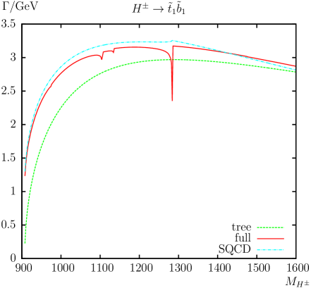
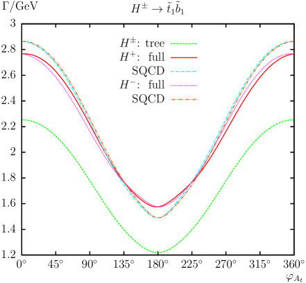
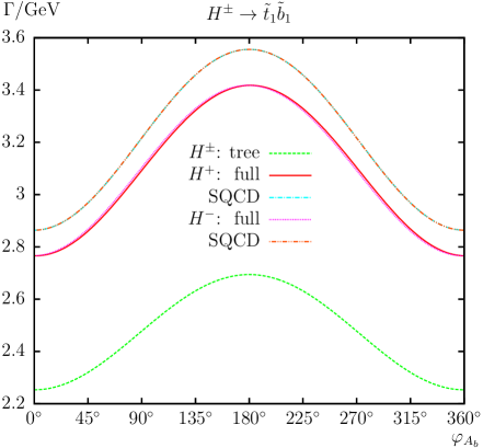
Figure 3: $\Gamma(H^{\pm}\to\tilde{t}_{1}\tilde{b}_{1})$. Tree-level, full and SQCD one-loop corrected partial decay widths are shown. The upper plot shows the partial decay width with $M_{H^{\pm}}$ varied. The lower plots show the complex phases $\varphi_{A_{t}}$ (left) and $\varphi_{A_{b}}$ (right) varied with parameters chosen according to S1 (see Tab. 1).

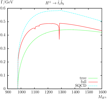
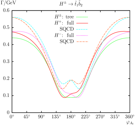
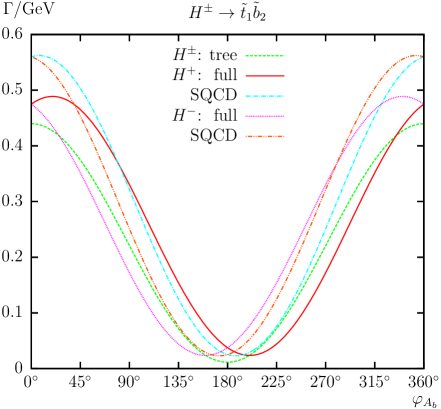
Figure 4: $\Gamma(H^{\pm}\to\tilde{t}_{1}\tilde{b}_{2})$. Tree-level, full and SQCD one-loop corrected partial decay widths are shown. The upper plot shows the partial decay width with $M_{H^{\pm}}$ varied. The lower plots show the complex phases $\varphi_{A_{t}}$ (left) and $\varphi_{A_{b}}$ (right) varied with parameters chosen according to S2 (see Tab. 1).

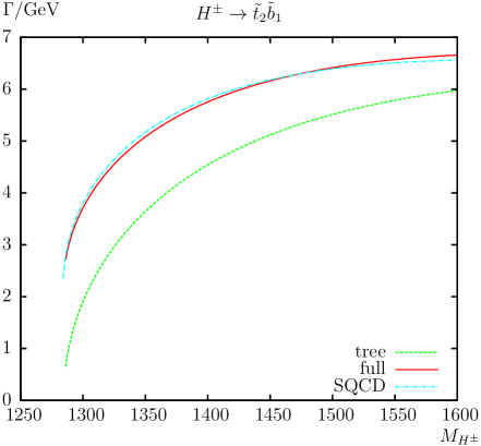
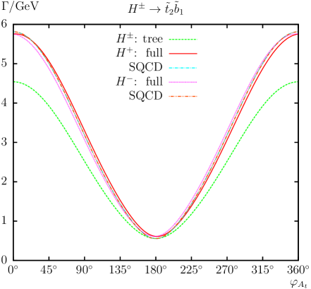
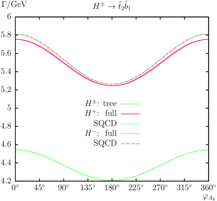
Figure 5: $\Gamma(H^{\pm}\to\tilde{t}_{2}\tilde{b}_{1})$. Tree-level, full and SQCD one-loop corrected partial decay widths are shown. The upper plot shows the partial decay width with $M_{H^{\pm}}$ varied. The lower plots show the complex phases $\varphi_{A_{t}}$ (left) and $\varphi_{A_{b}}$ (right) varied with parameters chosen according to S2 (see Tab. 1).

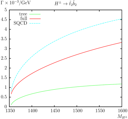
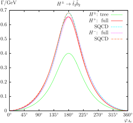
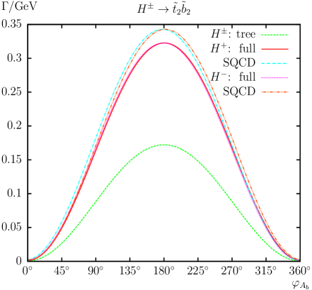
Figure 6: $\Gamma(H^{\pm}\to\tilde{t}_{2}\tilde{b}_{2})$. Tree-level, full and SQCD one-loop corrected partial decay widths are shown. The upper plot shows the partial decay width with $M_{H^{\pm}}$ varied. The lower plots show the complex phases $\varphi_{A_{t}}$ (left) and $\varphi_{A_{b}}$ (right) varied with parameters chosen according to S2 (see Tab. 1).

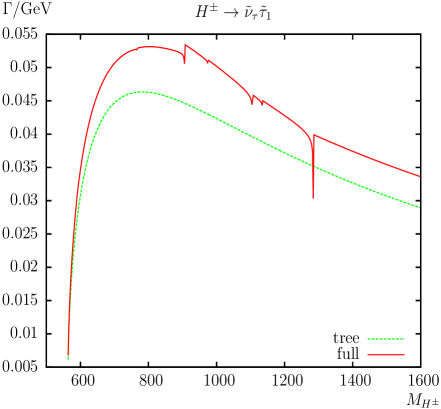
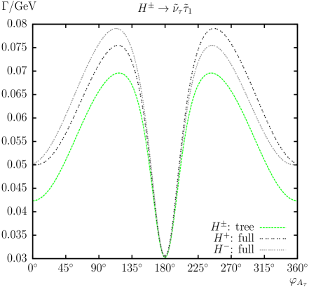
Figure 7: $\Gamma(H^{\pm}\to\tilde{\nu}_{\tau}\tilde{\tau}_{1})$. Tree-level and full one-loop corrected partial decay widths are shown. The left plot shows the partial decay width with $M_{H^{\pm}}$ varied; the right plot shows the complex phase $\varphi_{A_{\tau}}$ varied with parameters chosen according to S1 (see Tab. 1).

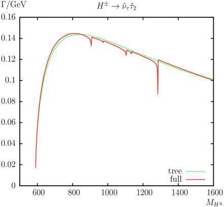
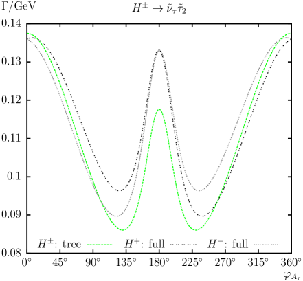
Figure 8: $\Gamma(H^{\pm}\to\tilde{\nu}_{\tau}\tilde{\tau}_{2})$. Tree-level and full one-loop corrected partial decay widths are shown. The left plot shows the partial decay width with $M_{H^{\pm}}$ varied; the right plot shows the complex phase $\varphi_{A_{\tau}}$ varied with parameters chosen according to S1 (see Tab. 1).

4.3.2 $h_{n}$ decays into sfermions

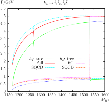
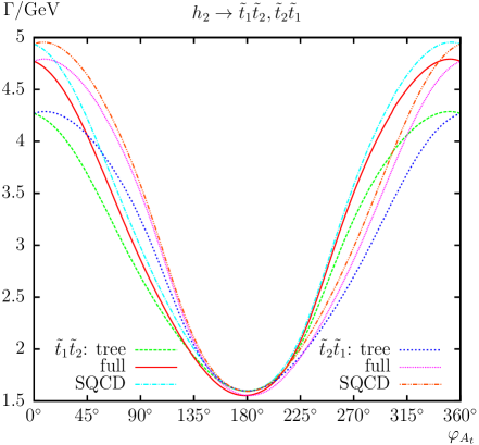
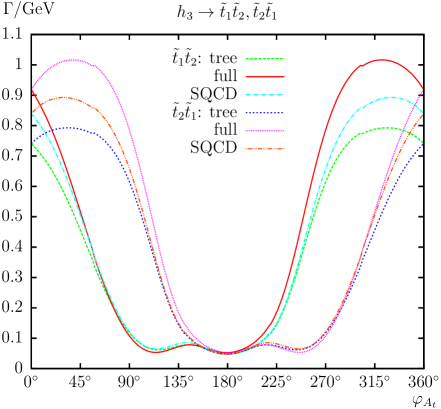
Figure 9: $\Gamma(h_{n}\to{\tilde{t}_{1}}{\tilde{t}_{2}},{\tilde{t}_{2}}{\tilde{t}_{1}})$. Tree-level, full and SQCD one-loop corrected partial decay widths are shown. The upper plot shows the partial decay width with $M_{H^{\pm}}$ varied; the lower plots show the complex phase $\varphi_{A_{t}}$ varied for $h_{2}$ decays (left) and $h_{3}$ decays (right) with parameters chosen according to S2 (see Tab. 1).

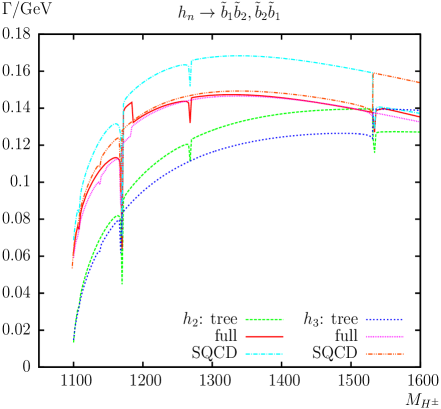
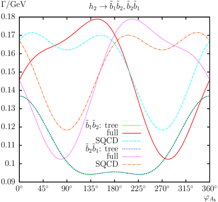
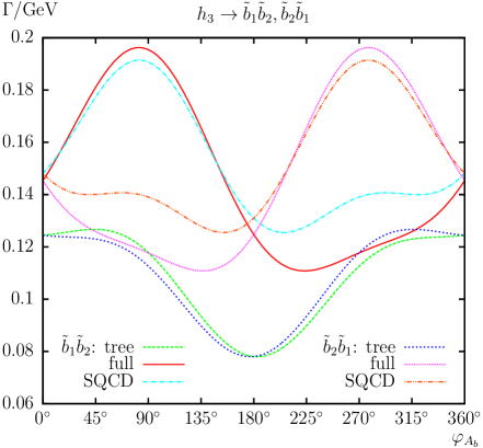
Figure 10: $\Gamma(h_{n}\to{\tilde{b}_{1}}{\tilde{b}_{2}},{\tilde{b}_{2}}{\tilde{b}_{1}})$. Tree-level, full and SQCD one-loop corrected partial decay widths are shown. The upper plot shows the partial decay width with $M_{H^{\pm}}$ varied; the lower plots show the complex phase $\varphi_{A_{b}}$ varied for $h_{2}$ decays (left) and $h_{3}$ decays (right) with parameters chosen according to S2 (see Tab. 1).

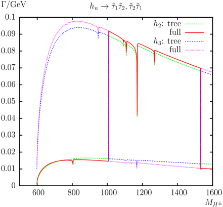
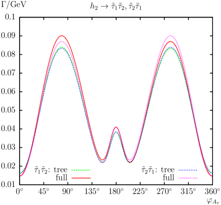
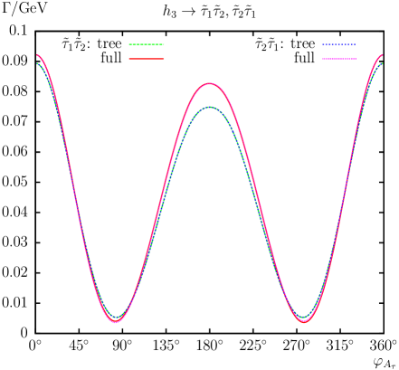
Figure 11: $\Gamma(h_{n}\to{\tilde{\tau}_{1}}{\tilde{\tau}_{2}},{\tilde{\tau}_{2}}{\tilde{\tau}_{1}})$. Tree-level and full one-loop corrected partial decay widths are shown. The upper plot shows the partial decay width with $M_{H^{\pm}}$ varied; the lower plots show the complex phase $\varphi_{A_{\tau}}$ varied for $h_{2}$ decays (left) and $h_{3}$ decays (right) with parameters chosen according to S1 (see Tab. 1).

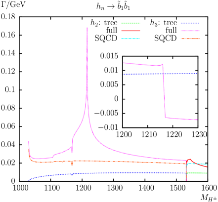
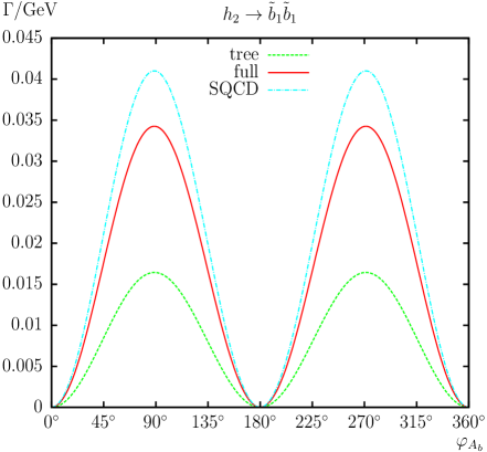
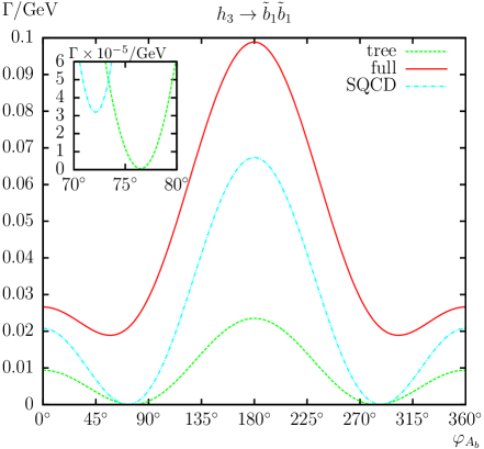
Figure 12: $\Gamma(h_{n}\to{\tilde{b}_{1}}{\tilde{b}_{1}})$. Tree-level, full and SQCD one-loop corrected partial decay widths are shown. The upper plot shows the partial decay width with $M_{H^{\pm}}$ varied; the lower plots show the complex phase $\varphi_{A_{b}}$ varied for $h_{2}$ decays (left) and $h_{3}$ decays (right) with parameters chosen according to S2 (see Tab. 1).

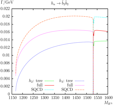
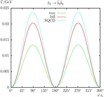
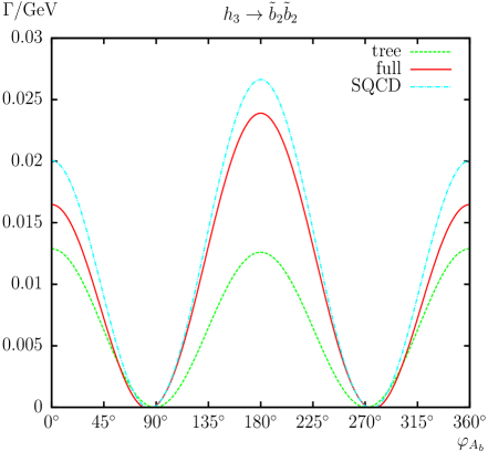
Figure 13: $\Gamma(h_{n}\to{\tilde{b}_{2}}{\tilde{b}_{2}})$. Tree-level, full and SQCD one-loop corrected partial decay widths are shown. The upper plot shows the partial decay width with $M_{H^{\pm}}$ varied; the lower plots show the complex phase $\varphi_{A_{b}}$ varied for $h_{2}$ decays (left) and $h_{3}$ decays (right) with parameters chosen according to S2 (see Tab. 1).

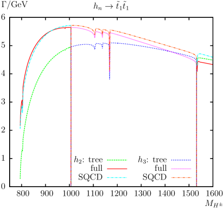
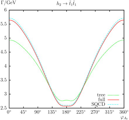
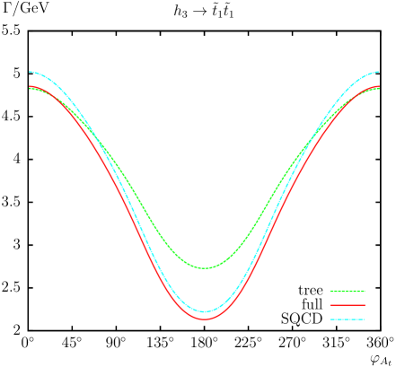
Figure 14: $\Gamma(h_{n}\to{\tilde{t}_{1}}{\tilde{t}_{1}})$. Tree-level, full and SQCD one-loop corrected partial decay widths are shown. The upper plot shows the partial decay width with $M_{H^{\pm}}$ varied; the lower plots show the complex phase $\varphi_{A_{b}}$ varied for $h_{2}$ decays (left, S1) and $h_{3}$ decays (right, S2).

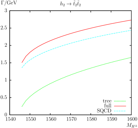
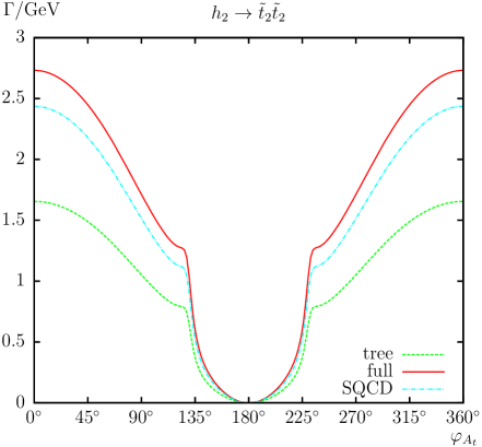
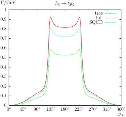
Figure 15: $\Gamma(h_{n}\to{\tilde{t}_{2}}{\tilde{t}_{2}})$. Tree-level, full and SQCD one-loop corrected partial decay widths are shown. The upper plot shows the partial decay width with $M_{H^{\pm}}$ varied; the lower plots show the complex phase $\varphi_{A_{t}}$ varied for $h_{2}$ decays (left) and $h_{3}$ decays (right) with parameters chosen according to S3 (see Tab. 1).

We now turn to the decay modes $h_{n}\to{\tilde{f}}_{i}{\tilde{f}}_{j}$ ($n=2,3;i,j=1,2$). Results are shown in the Figs. 9 – 18.

Before discussing every figure in detail, it should be noted that there is a subtleness concerning the mixture of the $h_{n}$ bosons. Depending on the input parameters, the higher-order corrections to the three neutral Higgs boson masses can vary substantially. The mass ordering $m_{h_{1}}<m_{h_{2}}<m_{h_{3}}$ (as performed automatically by FeynHiggs), even in the case of real parameters, can yield a heavy ${\cal CP}$-even Higgs mass higher or lower than the (heavy) ${\cal CP}$-odd Higgs mass. Such a transition in the mass ordering (or “mass crossing”) is accompanied by an abrupt change in the Higgs mixing matrix $\mathbf{\hat{Z}}$. For our input parameters (see Tab. 1) there are two (possible) crossings. The first (called “MC1” below) appears at $M_{H^{\pm}}\approx 1006\,\,\mathrm{GeV}$. Before the crossing we find $h_{2}\sim H$ ($h_{3}\sim A$), whereas after the crossing it changes to $h_{2}\sim A$ ($h_{3}\sim H$). The second crossing (called “MC2”) is found at $M_{H^{\pm}}\approx 1535\,\,\mathrm{GeV}$, i.e. the changing of the mixture from $h_{2}\sim A$ ($h_{3}\sim H$) to $h_{2}\sim H$ ($h_{3}\sim A$). Very close to the mass crossings the $\mathbf{\hat{Z}}$ matrix can yield small numerical instabilities. As an example, for $1534\,\,\mathrm{GeV}\lesssim M_{H^{\pm}}\lesssim 1536\,\,\mathrm{GeV}$ the $\mathbf{\hat{Z}}$ matrix causes structures appearing similar to “usual” dips from thresholds.

We start with the decay $h_{n}\to{\tilde{t}_{1}}{\tilde{t}_{2}},{\tilde{t}_{2}}{\tilde{t}_{1}}$ as shown in Fig. 9. The upper plot shows the results as a function of $M_{H^{\pm}}$, whereas in the lower plots we present the decay widths as a function of $\varphi_{A_{t}}$ in S2. We show separately the results for the $h_{2}$ and $h_{3}$ decay widths. In the upper plot of Fig. 9 the “apparently single” dip at $M_{H^{\pm}}\approx 1268\,\,\mathrm{GeV}$ is (again) in reality two dips coming from the thresholds $m_{\tilde{\chi}_{2}^{\pm}}+m_{\tilde{\chi}_{2}^{\pm}}=m_{h_{2}}\approx 1264\,\,\mathrm{GeV}$ and $m_{\tilde{\chi}_{4}^{0}}+m_{\tilde{\chi}_{4}^{0}}=m_{h_{2}}\approx 1265\,\,\mathrm{GeV}$. Away from the production threshold relative corrections of $\sim+12\%$ are found in S2 (see Tab. 1) for the $h_{2}$ decay. There the SQCD corrections overestimate the full correction by about $30\%$. In case of the $h_{3}$ decay the relative corrections are $\sim+24\%$ in S2 (see Tab. 1) and the SQCD corrections underestimate the full result by about $50\%$. The MC2 can be observed at $M_{H^{\pm}}\sim 1535\,\,\mathrm{GeV}$ as described above. Here $h_{2}$ and $h_{3}$ change their role. Within the unrotated scalar top basis the ${\cal CP}$-odd Higgs boson can only decay as $A\to\tilde{t}_{L}\tilde{t}_{R},\tilde{t}_{R}\tilde{t}_{L}$, but not as $A\to\tilde{t}_{L}\tilde{t}_{L},\tilde{t}_{R}\tilde{t}_{R}$, whereas the ${\cal CP}$-even Higgs boson has all four decays possible. Consequently, the decay to ${\tilde{t}_{1}}{\tilde{t}_{2}},{\tilde{t}_{2}}{\tilde{t}_{1}}$ can depend strongly on the ${\cal CP}$ nature of the decaying Higgs boson. While below MC2 we find $\Gamma(h_{2}\to{\tilde{t}_{1}}{\tilde{t}_{2}},{\tilde{t}_{2}}{\tilde{t}_{1}})\gg\Gamma(h_{3}\to{\tilde{t}_{1}}{\tilde{t}_{2}},{\tilde{t}_{2}}{\tilde{t}_{1}})$, above MC2 we have correspondingly $\Gamma(h_{2}\to{\tilde{t}_{1}}{\tilde{t}_{2}},{\tilde{t}_{2}}{\tilde{t}_{1}})\ll\Gamma(h_{3}\to{\tilde{t}_{1}}{\tilde{t}_{2}},{\tilde{t}_{2}}{\tilde{t}_{1}})$, as can be clearly observed in the upper plot of Fig. 9.

We now turn to the phase dependence of the decay width shown in S2, i.e. for $M_{H^{\pm}}=1400\,\,\mathrm{GeV}$, where the left (right) plot in Fig. 9 shows the dependence of $\Gamma(h_{2}\to{\tilde{t}_{1}}{\tilde{t}_{2}},{\tilde{t}_{2}}{\tilde{t}_{1}})$ ($\Gamma(h_{3}\to{\tilde{t}_{1}}{\tilde{t}_{2}},{\tilde{t}_{2}}{\tilde{t}_{1}})$) on $\varphi_{A_{t}}$. In the lower left plot one can observe that already the tree level result (green dashed) and the tree of the conjugated process (blue short dashed) are asymmetric and depend strongly on the phase. The assymetry at the tree-level is due to the contribution from the $\mathbf{\hat{Z}}$ matrix, which is not in general unitary and depends via the stop contributions to the Higgs boson self-energies on $\varphi_{A_{t}}$, see Ref. [17]. While for $\varphi_{A_{t}}\sim 180^{\circ}$ a width of about $1.5\,\,\mathrm{GeV}$ is observed, for $\varphi_{A_{t}}\sim 0^{\circ}$ a three times higher decay width is found. The full corrections for $\varphi_{A_{t}}$ varied are $\lesssim+12\%$ for S2, while the SQCD corrections overestimate the full corrections up to $30\%$. In the lower right plot of Fig. 9, where we show the $\varphi_{A_{t}}$ dependence of the $h_{3}$ decay one can see that as for the $h_{2}$ case already the tree level results (green dashed) and the tree of the conjugated process (blue short dashed) depend strongly on the phase and exhibit an asymmetry. The latter is again due to the contribution from the $\mathbf{\hat{Z}}$ matrix. The relative corrections for $\varphi_{A_{t}}$ are up to $\sim+29\%$ for S2. The SQCD corrections are smaller and would underestimate the full corrections by more than $50\%$.

In Fig. 10 we present the results for the decays $h_{n}\to{\tilde{b}_{1}}{\tilde{b}_{2}},{\tilde{b}_{2}}{\tilde{b}_{1}}$, where in the upper (lower) row we show the dependence on $M_{H^{\pm}}$ ($\varphi_{A_{b}}$). In the upper row plot the first “apparently single” dip in the $h_{2}$ decay (upper lines) is in reality two dips at $M_{H^{\pm}}\approx 1108\,\,\mathrm{GeV}$ and $M_{H^{\pm}}\approx 1112\,\,\mathrm{GeV}$ coming from the thresholds $m_{\tilde{\chi}_{1}^{\pm}}+m_{\tilde{\chi}_{2}^{\pm}}=m_{h_{2}}\approx 1105\,\,\mathrm{GeV}$ and $m_{\tilde{\chi}_{2}^{0}}+m_{\tilde{\chi}_{4}^{0}}=m_{h_{2}}\approx 1108\,\,\mathrm{GeV}$. The second dip at $M_{H^{\pm}}\approx 1171\,\,\mathrm{GeV}$ is the threshold $m_{\tilde{t}_{1}}+m_{\tilde{t}_{2}}=m_{h_{2}}=1165\,\,\mathrm{GeV}$. The “step” at $M_{H^{\pm}}\approx 1184\,\,\mathrm{GeV}$ could be traced back to the $C$-functions $C_{0,1,2}(m_{h_{2}}^{2},m_{\tilde{b}_{1}}^{2},m_{\tilde{b}_{2}}^{2},m_{\tilde{t}_{i}}^{2},m_{\tilde{t}_{j}}^{2},M_{W}^{2})$ with $i\neq j$ (but without any apparent threshold). The remaining dip (at $M_{H^{\pm}}\approx 1268\,\,\mathrm{GeV}$) is the same as in Fig. 9 for the same reasons (see above). At $M_{H^{\pm}}=1400\,\,\mathrm{GeV}$ the full one-loop corrections to the $h_{2}$ decay reach only $\sim+6\%$, while the SQCD corrections would overestimate this by a factor of $\sim 2.5$. Now we turn to the corresponing $h_{3}$ decay. The first three dips and the “step” at $M_{H^{\pm}}\approx 1182\,\,\mathrm{GeV}$ are the same as for the $h_{2}$ decay, see above. For the decay of the $h_{3}$ at $M_{H^{\pm}}=1400\,\,\mathrm{GeV}$ we find full corrections at the level of $+17\%$, where the SQCD results are only slightly larger. As in Fig. 9 one can observe the MC2 with an “interchange” of $h_{2}$ and $h_{3}$.

In the lower left plot of Fig. 10 we present $\Gamma(h_{2}\to{\tilde{b}_{1}}{\tilde{b}_{2}},{\tilde{b}_{2}}{\tilde{b}_{1}})$ as a function of $\varphi_{A_{b}}$ in S2. The variation with $\varphi_{A_{b}}$ is found to be very large, full relative corrections are up to $\sim+90\%$ for S2, where the SQCD corrections account for about $60\%$ of those. This can partially be attributed to the very small tree-level within the region $60^{\circ}\lesssim\varphi_{A_{b}}\lesssim 300^{\circ}$. Furthermore a very strong asymmetry between one decay and its complex conjugate can be observed, reaching up to $60\%$. In the lower right plot the corresponding results for the $h_{3}$ decay are shown. One can see that again already the tree level result (green dashed) and the tree of the conjugated process (blue short dashed) are asymmetric, which is caused again by the $\mathbf{\hat{Z}}$ matrix contribution, where $\varphi_{A_{b}}$ enters via the $\tilde{b}$ contributions to the Higgs-boson self-energies. As in the $h_{2}$ case the size of the corrections shows also a large variation with $\varphi_{A_{b}}$. The full relative corrections are up to $\sim+66\%$ for S2, where the SQCD corrections are only slightly smaller.

The third “mixed case”, the decays $h_{n}\to{\tilde{\tau}_{1}}{\tilde{\tau}_{2}},{\tilde{\tau}_{2}}{\tilde{\tau}_{1}}$, is shown in Fig. 11. As before, the upper plots depict the result as a function of $M_{H^{\pm}}$, whereas the lower row presents the $\varphi_{A_{\tau}}$ dependence. We start with the $h_{2}$ decay as a function of $M_{H^{\pm}}$. The first dip at $M_{H^{\pm}}\approx 805\,\,\mathrm{GeV}$ is the threshold $m_{\tilde{\chi}_{1}^{0}}+m_{\tilde{\chi}_{3}^{0}}=m_{h_{2}}\approx 799\,\,\mathrm{GeV}$. The second (small) dip at $M_{H^{\pm}}\approx 1092\,\,\mathrm{GeV}$ is the threshold $m_{\tilde{b}_{1}}+m_{\tilde{b}_{2}}=m_{h_{2}}\approx 1086\,\,\mathrm{GeV}$. The third “apparently single” dip is (again) in reality two dips at $M_{H^{\pm}}\approx 1108\,\,\mathrm{GeV}$ and $M_{H^{\pm}}\approx 1112\,\,\mathrm{GeV}$ coming from the thresholds $m_{\tilde{\chi}_{1}^{\pm}}+m_{\tilde{\chi}_{2}^{\pm}}=m_{h_{2}}\approx 1105\,\,\mathrm{GeV}$ and $m_{\tilde{\chi}_{2}^{0}}+m_{\tilde{\chi}_{4}^{0}}=m_{h_{2}}\approx 1108\,\,\mathrm{GeV}$. The fourth (large) dip at $M_{H^{\pm}}\approx 1171\,\,\mathrm{GeV}$ is (again) the threshold $m_{\tilde{t}_{1}}+m_{\tilde{t}_{2}}=m_{h_{2}}=1165\,\,\mathrm{GeV}$. The last dip (at $M_{H^{\pm}}\approx 1268\,\,\mathrm{GeV}$) is (again) the same as in Fig. 9 (see above). At $M_{H^{\pm}}=1000\,\,\mathrm{GeV}$ the full one-loop corrections reach $\sim-9\%$. In the same plot we show also the results for the $h_{3}$ decay. The first (small) dip in the upper plot at $M_{H^{\pm}}\approx 775\,\,\mathrm{GeV}$ is the threshold $m_{\tilde{\chi}_{1}^{0}}+m_{\tilde{\chi}_{2}^{0}}=m_{h_{3}}\approx 771\,\,\mathrm{GeV}$. The second dip is in reality two dips at $M_{H^{\pm}}\approx 948\,\,\mathrm{GeV}$ and $M_{H^{\pm}}\approx 954\,\,\mathrm{GeV}$ coming from the thresholds $m_{\tilde{\chi}_{1}^{\pm}}+m_{\tilde{\chi}_{1}^{\pm}}=m_{h_{3}}\approx 945\,\,\mathrm{GeV}$ and $m_{\tilde{\chi}_{2}^{0}}+m_{\tilde{\chi}_{2}^{0}}=m_{h_{3}}\approx 951\,\,\mathrm{GeV}$. The third dip is (again) at $M_{H^{\pm}}\approx 1108\,\,\mathrm{GeV}$ coming from the threshold $m_{\tilde{\chi}_{1}^{\pm}}+m_{\tilde{\chi}_{2}^{\pm}}=m_{h_{3}}\approx 1105\,\,\mathrm{GeV}$. The fourth dip at $M_{H^{\pm}}\approx 1138\,\,\mathrm{GeV}$ is (again) the threshold $m_{\tilde{\chi}_{3}^{0}}+m_{\tilde{\chi}_{4}^{0}}=m_{h_{3}}=1135\,\,\mathrm{GeV}$. The fifth (large) dip at $M_{H^{\pm}}\approx 1168\,\,\mathrm{GeV}$ is (again) the threshold $m_{\tilde{t}_{1}}+m_{\tilde{t}_{2}}=m_{h_{3}}\approx 1165\,\,\mathrm{GeV}$. At $M_{H^{\pm}}=1000\,\,\mathrm{GeV}$ the full one-loop corrections reach $\sim+3\%$. The two mass crossings, MC1 and MC2, can again be observed, where $h_{2}$ and $h_{3}$ interchange their ${\cal CP}$ character.

We now turn to the results for the $h_{2}\ (h_{3})$ decay as a function of $\varphi_{A_{\tau}}$ in the lower left (right) plot of Fig. 11. For the $h_{2}$ decay the relative corrections for $\varphi_{A_{\tau}}=80^{\circ},180^{\circ},280^{\circ}$ are up to $\sim+7\%$ in S1. For the $h_{3}$ decay, on the other hand, the relative corrections for $\varphi_{A_{\tau}}=82^{\circ},180^{\circ}$ are up to $\sim-24\%,\sim+10\%$ in S1. The asymmetry is to small to be visible in the plot.

Next we consider $h_{n}$ decays into sfermions with equal sfermion indices and it should be noted that the $A{\tilde{f}}_{i}{\tilde{f}}_{i}$ ($i=1,2$) couplings are exactly zero in case of real input parameters.

In Fig. 12 we present the results for the decays $h_{n}\to{\tilde{b}_{1}}{\tilde{b}_{1}}$. The dependence on $M_{H^{\pm}}$ is shown in the upper plot, whereas the dependence on $\varphi_{A_{b}}$ for $M_{H^{\pm}}=1400\,\,\mathrm{GeV}$ is given in the lower plots. We start with $\Gamma(h_{2}\to{\tilde{b}_{1}}{\tilde{b}_{1}})$ in the upper plot. Only above MC2 this decay width becomes non-zero. The peak at $M_{H^{\pm}}\approx 1545\,\,\mathrm{GeV}$ (red line) is the threshold $m_{\tilde{t}_{2}}+m_{\tilde{t}_{2}}=m_{h_{2}}=1542\,\,\mathrm{GeV}$. Furthermore the tree level decay width $\Gamma(h_{2}\to{\tilde{b}_{1}}{\tilde{b}_{1}})$ is accidently very small for the parameter set chosen, see Tab. 1. Because of this smallness, the relative size of the one-loop correction becomes larger then the tree level, and can even turn negative. Therefore in this case we added $|{\cal M}_{\text{loop}}|^{2}$ to the full one-loop result to obtain a positive decay width. The full relative corrections are $\sim+73\%$ at $M_{H^{\pm}}=1600\,\,\mathrm{GeV}$ and the SQCD corrections are $\sim+80\%$. Also shown in this plot is the decay $h_{3}\to{\tilde{b}_{1}}{\tilde{b}_{1}}$, which is non-zero below MC2. The first dip at $M_{H^{\pm}}\approx 1108\,\,\mathrm{GeV}$ is the threshold $m_{\tilde{\chi}_{1}^{\pm}}+m_{\tilde{\chi}_{2}^{\pm}}=m_{h_{3}}\approx 1105\,\,\mathrm{GeV}$. The second dip (not visible) at $M_{H^{\pm}}\approx 1138\,\,\mathrm{GeV}$ is the threshold $m_{\tilde{\chi}_{3}^{0}}+m_{\tilde{\chi}_{4}^{0}}=m_{h_{3}}=1135\,\,\mathrm{GeV}$. The third dip at $M_{H^{\pm}}\approx 1168\,\,\mathrm{GeV}$ is the threshold $m_{\tilde{t}_{1}}+m_{\tilde{t}_{2}}=m_{h_{3}}=1165\,\,\mathrm{GeV}$. The large “spike” at $M_{H^{\pm}}\approx 1216\,\,\mathrm{GeV}$ is caused by the addition of the two-loop contribution $|{\cal M}_{\text{loop}}|^{2}$ as explained above (formally it is caused by the $C$-functions $C_{0,1,2}(m_{h_{3}}^{2},m_{\tilde{b}_{1}}^{2},m_{\tilde{b}_{1}}^{2},m_{\tilde{t}_{i}}^{2},m_{\tilde{t}_{j}}^{2},M_{W}^{2})$ with $i\neq j$). Without the two-loop contribution it appears as “step” (see the inlay in the upper plot of Fig. 12) similar to Fig. 10. Because of the smallness of the tree, the full relative corrections reach $\sim+183\%$ at $M_{H^{\pm}}=1400\,\,\mathrm{GeV}$. Here the SQCD corrections are smaller with $\sim+92\%$.

In the lower left plot of Fig. 12 we show the $h_{2}$ decay with the complex phase $\varphi_{A_{b}}$ varied at $M_{H^{\pm}}=1400\,\,\mathrm{GeV}$. For $\varphi_{A_{b}}=0^{\circ},180^{\circ},360^{\circ}$, i.e. real parameters the $h_{2}$ decay is purely ${\cal CP}$-odd, and thus the decay width is zero. For complex values of the phase small, but non-zero values are reached. Here, for the same reasons as in the upper plot the loop corrections can be larger then the tree level and reach actually $\sim+108\%$ (and $\sim+125\%$ for SQCD) at $\varphi_{A_{b}}=90^{\circ},270^{\circ}$. In the lower right plot of Fig. 12 we show the $h_{3}$ decay with the complex phase $\varphi_{A_{b}}$ varied at $M_{H^{\pm}}=1400\,\,\mathrm{GeV}$. Here (for the same reasons as in the upper plot) the loop corrections can be larger then the tree level (and for consistency with the upper plot we also add $|{\cal M}_{\text{loop}}|^{2}$ here) and reach up to $\sim+320\%$ (and $\sim+165\%$ for SQCD) at $\varphi_{A_{b}}=180^{\circ}$. It should be noted that the decay width including SQCD corrections does not go to zero due to $|{\cal M}_{\text{loop}}|^{2}$, but just reaches a (very) small value of $\Gamma(h_{3}\to{\tilde{b}_{1}}{\tilde{b}_{1}})$ (see the inlay in the lower right plot of Fig. 12).

In Fig. 13 we present the decay $h_{n}\to{\tilde{b}_{2}}{\tilde{b}_{2}}$, in full analogy to Fig. 12. The same behavior of $h_{2}$ and $h_{3}$ concerning MC2 can be observed. The full relative corrections for the $h_{2}$ decay are $\sim+18\%$ at $M_{H^{\pm}}=1600\,\,\mathrm{GeV}$, where the pure SQCD corrections would overestimate this correction by a factor $\sim 1.8$. The decay $h_{3}\to{\tilde{b}_{2}}{\tilde{b}_{2}}$ is again non-zero only below MC2. The dip (hardly visible) at $M_{H^{\pm}}\approx 1168\,\,\mathrm{GeV}$ in the $h_{3}$ decay is the threshold $m_{\tilde{t}_{1}}+m_{\tilde{t}_{2}}=m_{h_{3}}=1165\,\,\mathrm{GeV}$. The full relative corrections are $\sim+28\%$ at $M_{H^{\pm}}=1400\,\,\mathrm{GeV}$ and the SQCD corrections are larger by about a factor of 1.6. In the lower left plot of Fig. 13 we show the variation of $\Gamma(h_{2}\to{\tilde{b}_{2}}{\tilde{b}_{2}})$ with $\varphi_{A_{b}}$ at $M_{H^{\pm}}=1400\,\,\mathrm{GeV}$. Here the loop corrections reach $\sim+52\%$ (and $\sim+60\%$ for SQCD) at $\varphi_{A_{b}}=90^{\circ},270^{\circ}$. The decay width goes to zero for real $A_{b}$ due to the ${\cal CP}$-nature of the $h_{2}$. In the lower right plot of Fig. 13 we show $\Gamma(h_{3}\to{\tilde{b}_{2}}{\tilde{b}_{2}})$ with $\varphi_{A_{b}}$ varied at $M_{H^{\pm}}=1400\,\,\mathrm{GeV}$. Here the loop corrections reach $\sim+90\%$ at $\varphi_{A_{b}}=180^{\circ}$ and are slightly overestimated in the pure SQCD case. The decay width goes to zero for $\varphi_{A_{b}}\sim 85^{\circ},275^{\circ}$. For these values the relevant diagonal entries of the $\mathbf{\hat{Z}}$ matrix go through zero, i.e. the main effect on the decay width stems from the $\mathbf{\hat{Z}}$ matrix.

We now turn to the neutral Higgs decay to scalar top quarks, which are shown in full analogy to the decay to scalar bottom quarks above. In Fig. 14 we present the decay $h_{n}\to{\tilde{t}_{1}}{\tilde{t}_{1}}$. In the upper row we show the results as a function of $M_{H^{\pm}}$. The first dip at $M_{H^{\pm}}\approx 805\,\,\mathrm{GeV}$ in the $h_{2}$ decay is the threshold $m_{\tilde{\chi}_{1}^{0}}+m_{\tilde{\chi}_{3}^{0}}=m_{h_{2}}\approx 799\,\,\mathrm{GeV}$. The second dip at $M_{H^{\pm}}\approx 982\,\,\mathrm{GeV}$ is the threshold $m_{\tilde{\chi}_{2}^{0}}+m_{\tilde{\chi}_{3}^{0}}=m_{h_{2}}\approx 979\,\,\mathrm{GeV}$. The full relative corrections are $\sim+14\%$ at $M_{H^{\pm}}=1000\,\,\mathrm{GeV}$ (i.e. S1) and the SQCD corrections are $\sim+16\%$. The decay width turns zero between MC1 and MC2 and reaches non-zero values below MC1 and above MC2. Reversely, we find non-zero values for $\Gamma(h_{3}\to{\tilde{t}_{1}}{\tilde{t}_{1}})$ only between MC1 and MC2. The first dip at $M_{H^{\pm}}\approx 1108\,\,\mathrm{GeV}$ in the $h_{3}$ decay is the threshold $m_{\tilde{\chi}_{1}^{\pm}}+m_{\tilde{\chi}_{2}^{\pm}}=m_{h_{3}}1105\approx\,\,\mathrm{GeV}$. The second dip at $M_{H^{\pm}}\approx 1138\,\,\mathrm{GeV}$ is the threshold $m_{\tilde{\chi}_{3}^{0}}+m_{\tilde{\chi}_{4}^{0}}=m_{h_{3}}\approx 1135\,\,\mathrm{GeV}$. The third dip at $M_{H^{\pm}}\approx 1168\,\,\mathrm{GeV}$ is the threshold $m_{\tilde{t}_{1}}+m_{\tilde{t}_{2}}=m_{h_{3}}=1165\,\,\mathrm{GeV}$. The full relative corrections at $M_{H^{\pm}}=1400\,\,\mathrm{GeV}$ are accidentally small and reach only $+1\%$, where the pure SQCD corrections reach $\sim+4\%$. In the lower left plot of Fig. 14 we show the $h_{2}$ decay with the complex phase $\varphi_{A_{t}}$ varied at $M_{H^{\pm}}=1000\,\,\mathrm{GeV}$. Here the loop corrections can vary between $\sim+14\%$ for $\varphi_{A_{t}}\sim 0^{\circ},360^{\circ}$ and $\sim-7\%$ at $\varphi_{A_{t}}=180^{\circ}$, where the SQCD corrections in this case are a good approximation to the full result. In the lower right plot of Fig. 14 we show the $h_{3}$ decay with $\varphi_{A_{t}}$ varied at $M_{H^{\pm}}=1400\,\,\mathrm{GeV}$. Here the loop corrections are close to zero for real positive values of $A_{b}$, where the EW corrections compensate the SQCD contributions. The full corrections can reach $\sim-22\%$ (and $\sim-19\%$ for SQCD) at $\varphi_{A_{t}}=180^{\circ}$.

The final decays involving stops are shown in Fig. 15. The results as a function of $M_{H^{\pm}}$ are given in the upper plot. Due to the large values of $m_{\tilde{t}_{2}}$ for real parameters only $\Gamma(h_{2}\to{\tilde{t}_{2}}{\tilde{t}_{2}})$ reaches non-zero values. The full relative corrections for the $h_{2}$ decay are $\sim+65\%$ at $M_{H^{\pm}}=1600\,\,\mathrm{GeV}$ (i.e. S3) and the SQCD corrections reach $\sim+47\%$. In the lower left plot of Fig. 15 we show $\Gamma(h_{2}\to{\tilde{t}_{2}}{\tilde{t}_{2}})$ with the complex phase $\varphi_{A_{t}}$ varied at $M_{H^{\pm}}=1600\,\,\mathrm{GeV}$. The smooth structure around $\varphi_{A_{t}}=130^{\circ},230^{\circ}$ is not a threshold but a numerical effect of the $\mathbf{\hat{Z}}$ matrix contribution. The loop corrections can reach $\sim+63\%$ (and $\sim+44\%$ for SQCD) at $\varphi_{A_{t}}=90^{\circ},270^{\circ}$. For $\varphi_{A_{t}}=180^{\circ}$ the decay width goes to zero since the relevant diagonal entries in the $\mathbf{\hat{Z}}$ matrix go through zero, see also the discussion of Fig. 13. The $h_{3}$ decay is non-zero above MC2 only for complex parameters. In the lower right plot of Fig. 15 we show $\Gamma(h_{3}\to{\tilde{t}_{2}}{\tilde{t}_{2}})$ with $\varphi_{A_{t}}$ varied at $M_{H^{\pm}}=1600\,\,\mathrm{GeV}$. The smooth structure around $\varphi_{A_{t}}=135^{\circ},225^{\circ}$ is again a numerical effect of the $\mathbf{\hat{Z}}$ matrix contribution. The loop corrections can reach $\sim+54\%$ (and $\sim+37\%$ for SQCD) at $\varphi_{A_{t}}=180^{\circ}$.

We finish our numerical analysis with the remaining decays to scalar leptons. In Fig. 16 the decay widths for $h_{n}\to\tilde{\nu}_{\tau}\tilde{\nu}_{\tau}$ are shown. In the upper plot the results as a function of $M_{H^{\pm}}$ are given. The decay $h_{2}\to\tilde{\nu}_{\tau}\tilde{\nu}_{\tau}$ for real parameters is non-zero below MC1 and above MC2 due to the ${\cal CP}$-structure of $h_{2}$. The first dip in the $h_{2}$ decay at $M_{H^{\pm}}\approx 598\,\,\mathrm{GeV}$ is the threshold $m_{\tilde{\chi}_{1}^{0}}+m_{\tilde{\chi}_{1}^{0}}=m_{h_{2}}\approx 591\,\,\mathrm{GeV}$. The second dip at $M_{H^{\pm}}\approx 624\,\,\mathrm{GeV}$ is the threshold $m_{\tilde{\tau}_{2}}+m_{\tilde{\tau}_{2}}=m_{h_{2}}=618\,\,\mathrm{GeV}$. The third dip at $M_{H^{\pm}}\approx 794\,\,\mathrm{GeV}$ is the threshold $m_{\tilde{t}_{1}}+m_{\tilde{t}_{1}}=m_{h_{2}}=788\,\,\mathrm{GeV}$. The fourth dip at $M_{H^{\pm}}\approx 805\,\,\mathrm{GeV}$ is the threshold $m_{\tilde{\chi}_{1}^{0}}+m_{\tilde{\chi}_{3}^{0}}=m_{h_{2}}\approx 799\,\,\mathrm{GeV}$. The last dip (hardly visible) at $M_{H^{\pm}}\approx 982\,\,\mathrm{GeV}$ is the threshold $m_{\tilde{\chi}_{2}^{0}}+m_{\tilde{\chi}_{3}^{0}}=m_{h_{2}}\approx 979\,\,\mathrm{GeV}$. The full relative corrections are found to be $\sim-48\%$ at $M_{H^{\pm}}=1000\,\,\mathrm{GeV}$ (i.e. S1). Correspondingly, the decay $h_{3}\to\tilde{\nu}_{\tau}\tilde{\nu}_{\tau}$ for real parameters is non-zero only between MC1 and MC2. The first dip at $M_{H^{\pm}}\approx 1108\,\,\mathrm{GeV}$ is (again) the threshold $m_{\tilde{\chi}_{1}^{\pm}}+m_{\tilde{\chi}_{2}^{\pm}}=m_{h_{3}}1105\approx\,\,\mathrm{GeV}$. The second dip at $M_{H^{\pm}}\approx 1138\,\,\mathrm{GeV}$ is (again) the threshold $m_{\tilde{\chi}_{3}^{0}}+m_{\tilde{\chi}_{4}^{0}}=m_{h_{3}}\approx 1135\,\,\mathrm{GeV}$. The third dip at $M_{H^{\pm}}\approx 1168\,\,\mathrm{GeV}$ is (again) the threshold $m_{\tilde{t}_{1}}+m_{\tilde{t}_{2}}=m_{h_{3}}=1165\,\,\mathrm{GeV}$. The full relative corrections are $\sim-17\%$ at $M_{H^{\pm}}=1400\,\,\mathrm{GeV}$ (i.e. S2). The dependence on $\varphi_{A_{\tau}}$ is shown for the $h_{2}\ (h_{3})$ decay in the lower left (right) plot of Fig. 16 for $M_{H^{\pm}}=1000\ (1400)\,\,\mathrm{GeV}$. For the $h_{2}$ decay the loop corrections can reach $\sim-40\%$ at $\varphi_{A_{\tau}}=180^{\circ}$. For the $h_{3}$ decay they can reach $\sim-12\%$ at $\varphi_{A_{\tau}}=180^{\circ}$.

In Fig. 17 we present the results for the decays $h_{n}\to{\tilde{\tau}_{1}}{\tilde{\tau}_{1}}$. The upper row shows the decay widths as a function of $M_{H^{\pm}}$. As before, the decay width of $h_{2}$ is non-zero for real parameters only below MC1 and above MC2, whereas the $h_{3}$ decay width is non-zero between the two mass crossing points. Starting with $h_{2}$, the first (large) dip at $M_{H^{\pm}}\approx 805\,\,\mathrm{GeV}$ in the $h_{2}$ decay is (again) the threshold $m_{\tilde{\chi}_{1}^{0}}+m_{\tilde{\chi}_{3}^{0}}=m_{h_{2}}\approx 799\,\,\mathrm{GeV}$. The second dip (hardly visible) at $M_{H^{\pm}}\approx 982\,\,\mathrm{GeV}$ is (again) the threshold $m_{\tilde{\chi}_{2}^{0}}+m_{\tilde{\chi}_{3}^{0}}=m_{h_{2}}\approx 979\,\,\mathrm{GeV}$. The full relative corrections are $\sim+8\%$ at $M_{H^{\pm}}=1000\,\,\mathrm{GeV}$ (i.e. S1). The three dips of the $h_{3}$ decay are the same as in the upper plot of Fig. 16, see above. The full relative corrections at $M_{H^{\pm}}=1400\,\,\mathrm{GeV}$ (i.e. S2) are $\sim+8\%$. In the lower left plot of Fig. 17 we show the $h_{2}$ decay with $\varphi_{A_{\tau}}$ varied at $M_{H^{\pm}}=1000\,\,\mathrm{GeV}$. Here the loop corrections can reach $\sim+9\%$ around $\varphi_{A_{\tau}}\sim 140^{\circ},220^{\circ}$. For $\varphi_{A_{\tau}}\sim 80^{\circ},280^{\circ}$ we find again the dominant effects from the $\mathbf{\hat{Z}}$ matrix, leading to a vanishing decay width around these values. In the lower right plot of Fig. 17 we show $h_{3}$ results as a function of $\varphi_{A_{\tau}}$ with $M_{H^{\pm}}=1400\,\,\mathrm{GeV}$. Here the loop corrections can reach $\sim+13\%$ at $\varphi_{A_{\tau}}\sim 140^{\circ},220^{\circ}$, and the $\mathbf{\hat{Z}}$ matrix causes the vanishing width around $\varphi_{A_{\tau}}\sim 80^{\circ},280^{\circ}$.

Finally, in Fig. 18 we present the results for $\Gamma(h_{n}\to{\tilde{\tau}_{2}}{\tilde{\tau}_{2}})$, which are shown in full analogy to $\Gamma(h_{n}\to{\tilde{\tau}_{1}}{\tilde{\tau}_{1}})$ above. As before, for real parameters, the $h_{2}$ decay width is found non-zero only below MC1 and above MC2, while the $h_{3}$ width is non-zero only between MC1 and MC2. The $h_{n}$ decay widths as a function of $M_{H^{\pm}}$ exhibit the same dips as in Fig. 17, see above. The full relative corrections to the $h_{2}$ width are $\sim+6\%$ at $M_{H^{\pm}}=1000\,\,\mathrm{GeV}$ (i.e. S1). The full relative corrections to the $h_{3}$ decay at $M_{H^{\pm}}=1400\,\,\mathrm{GeV}$ (i.e. S2) are $\sim+8\%$. In the lower left plot of Fig. 18 we show the $h_{2}$ decay with $\varphi_{A_{\tau}}$ varied at $M_{H^{\pm}}=1000\,\,\mathrm{GeV}$. Here the loop corrections can reach $\sim+12\%$ at $\varphi_{A_{\tau}}\sim 140^{\circ},180^{\circ},220^{\circ}$. The decay width goes to zero in analogy to Fig. 17. In the right plot of Fig. 18 the corresponding $h_{3}$ results are shown for $M_{H^{\pm}}=1400\,\,\mathrm{GeV}$, where we find the same level of higher-order corrections, and the dominating effect of the $\mathbf{\hat{Z}}$ matrix as in Fig. 17.

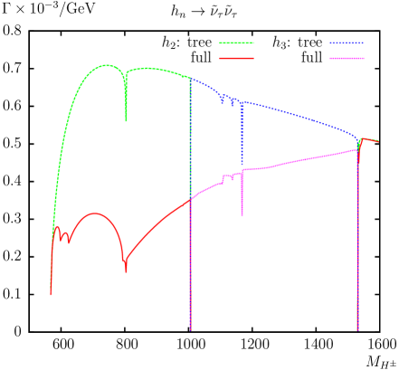
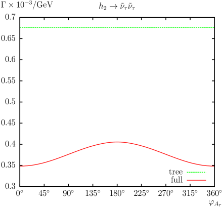
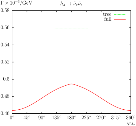
Figure 16: $\Gamma(h_{n}\to{\tilde{\nu}}_{\tau}{\tilde{\nu}}_{\tau})$. Tree-level and full one-loop corrected partial decay widths are shown. The upper plot shows the partial decay width with $M_{H^{\pm}}$ varied; the lower plots show the complex phase $\varphi_{A_{\tau}}$ varied for $h_{2}$ decays (left, S1) and $h_{3}$ decays (right, S2).

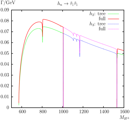
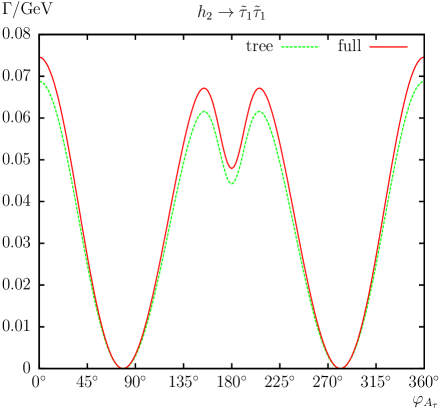
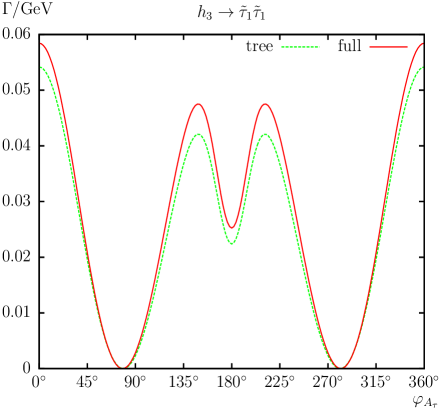
Figure 17: $\Gamma(h_{n}\to{\tilde{\tau}_{1}}{\tilde{\tau}_{1}})$. Tree-level and full one-loop corrected partial decay widths are shown. The upper plot shows the partial decay width with $M_{H^{\pm}}$ varied; the lower plots show the complex phase $\varphi_{A_{\tau}}$ varied for $h_{2}$ decays (left, S1) and $h_{3}$ decays (right, S2).

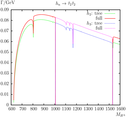
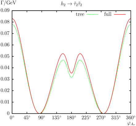
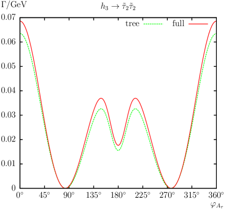
Figure 18: $\Gamma(h_{n}\to{\tilde{\tau}_{2}}{\tilde{\tau}_{2}})$. Tree-level and full one-loop corrected partial decay widths are shown. The upper plot shows the partial decay width with $M_{H^{\pm}}$ varied; the lower plots show the complex phase $\varphi_{A_{\tau}}$ varied for $h_{2}$ decays (left, S1) and $h_{3}$ decays (right, S2).

5 Conclusions

We evaluated all partial decay widths corresponding to a two-body decay of the heavy MSSM Higgs bosons to scalar fermions, allowing for complex parameters. The decay modes are given in Eqs. (1) and (2). The evaluation is based on a full one-loop calculation of all decay channels, also including hard QED and QCD radiation. In the case of a discovery of additional Higgs bosons a subsequent precision measurement of their properties will be crucial determine their nature and the underlying (SUSY) parameters. In order to yield a sufficient accuracy, one-loop corrections to the various Higgs-boson decay modes have to be considered. With the here presented full one-loop calculation to scalar fermions another step in the direction of a complete one-loop evaluation of all possible decay modes has been taken.

We first reviewed the one-loop renormalization procedure of the cMSSM, which is relevant for our calculation. In most cases we follow Ref. [37]. However, in the scalar fermion sector, where we differ from Ref. [37] all relevant details are given.

We have discussed the calculation of the one-loop diagrams, the treatment of UV and IR divergences that are canceled by the inclusion of (hard and soft) QCD and QED radiation. We have checked our result against the literature (where loop corrections so far only for real parameters were available) and in most cases found good agreement, once our set-up was changed to the one used in the existing analyses.

While the analytical calculation has been performed for all decay modes to sfermions, in the numerical analysis we concentrated on the decays to the third generation sfermions: scalar tops, bottoms, taus and tau neutrinos. For the analysis we have chosen a parameter set that allows simultaneously a maximum number of two-body sfermionic decay modes. In the analysis either the charged Higgs boson mass or the phase of a relevant trilinear coupling has been varied. For $M_{H^{\pm}}$ we investigated an interval starting at $M_{H^{\pm}}=600\,\,\mathrm{GeV}$ up to $M_{H^{\pm}}=1.6\,\,\mathrm{TeV}$, which roughly coincides with the reach of the LHC for high-luminosity running as well as an $e^{+}e^{-}$ collider with a center-of-mass energy up to $\sqrt{s}\sim 3\,\,\mathrm{TeV}$.

In our numerical scenarios we compared the tree-level partial decay widths with the full one-loop corrected partial decay widths. In the case of decays to scalar quarks we also included for comparison the pure SQCD one-loop corrections. We concentrated on the analysis of the decay widths themselves, since the size of the corresponding branching ratios (and thus the size of the one-loop effects) is highly parameter dependent.

We found sizable, roughly ${\cal O}(15\%)$, corrections in all the channels. The corrections tend to be larger for the decays to scalar quarks w.r.t. decays to scalar leptons. For some parts of the parameter space (not only close to thresholds) also larger corrections up to $30\%$ or $40\%$ (and in exceptional cases even higher) have been observed. Consequently, the full one-loop corrections should be taken into account for the interpretation of the searches for scalar fermions as well as for any future precision analyses of those decays.

The size of the tree-level decay widths and of the corresponding full one-loop corrections often depend strongly on the respective complex phase, i.e. $\varphi_{A_{t}},\varphi_{A_{b}}$ or $\varphi_{A_{\tau}}$. The one-loop contributions often vary by a factor of $2-3$ as a function of the complex phases and sometimes can even turn negative. Neglecting the phase dependence could lead to a wrong impression of the relative size of the various decay widths. Furthermore, for certain values of the phases the relevant diagonal entries in the $\mathbf{\hat{Z}}$ matrix go through zero. Consequently, also the decay widths go to zero for these values, where the $\mathbf{\hat{Z}}$ matrix yields the dominating effect on the widths.

In case of decays to scalar quarks we have also compared with the pure SQCD result. We have found that in most cases the EW corrections are of similar size. Neglecting those can lead, depending on the parameter space, to a large over- or underestimate of the full one-loop corrections.

In the cases where a decay and its complex conjugate final state are possible we have evaluated both decay widths independently. The asymmetries, as a byproduct of our calculation, turn out to be sizable, in particular for decays into a pair of lighter and heavier scalar fermions.

The numerical results we have shown are, of course, dependent on the choice of the SUSY parameters. Nevertheless, they give an idea of the relevance of the full one-loop corrections. Decay channels (and their respective one-loop corrections) that may look unobservable due to the smallness of their decay width in our numerical examples could become important if other channels are kinematically forbidden. Following our analysis it is evident that the full one-loop corrections are mandatory for a precise prediction of the various branching ratios. We emphasize again that in many cases it is not sufficient to include only SQCD corrections, as electroweak corrections can be of comparable size. The full one-loop corrections should be taken into account in any precise determination of (SUSY) parameters from the decay of heavy MSSM Higgs bosons. The results for the heavy MSSM Higgs decays will be implemented into the Fortran code FeynHiggs.

Acknowledgements

We thank T. Hahn, W. Hollik, H. Rzehak, and G. Weiglein for helpful discussions. The work of S.H. is supported in part by CICYT (grant FPA 2013-40715-P) and by the Spanish MICINN’s Consolider-Ingenio 2010 Program under grant MultiDark CSD2009-00064.

References

-
[1]
H. Nilles,
Phys. Rept. 110 (1984) 1;
R. Barbieri, Riv. Nuovo Cim. 11 (1988) 1. - [2] H. Haber, G. Kane, Phys. Rept. 117 (1985) 75.
- [3] J. Gunion, H. Haber, Nucl. Phys. B 272 (1986) 1.
- [4] G. Aad et al. [ATLAS Collaboration], Phys. Lett. B 716 (2012) 1 [arXiv:1207.7214 [hep-ex]].
- [5] S. Chatrchyan et al. [CMS Collaboration], Phys. Lett. B 716 (2012) 30 [arXiv:1207.7235 [hep-ex]].
- [6] H. Baer et al., The International Linear Collider Technical Design Report - Volume 2: Physics, arXiv:1306.6352 [hep-ph].
-
[7]
TESLA Technical Design Report [TESLA Collaboration] Part 3,
Physics at an Linear Collider,
arXiv:hep-ph/0106315,
see:
tesla.desy.de/new_pages/TDR_CD/start.html;
K. Ackermann et al., DESY-PROC-2004-01. -
[8]
J. Brau et al. [ILC Collaboration],
ILC Reference Design Report Volume 1 - Executive Summary,
arXiv:0712.1950 [physics.acc-ph];
G. Aarons et al. [ILC Collaboration], International Linear Collider Reference Design Report Volume 2: Physics at the ILC, arXiv:0709.1893 [hep-ph]. -
[9]
L. Linssen, A. Miyamoto, M. Stanitzki and H. Weerts,
arXiv:1202.5940 [physics.ins-det];
H. Abramowicz et al. [CLIC Detector and Physics Study Collaboration], Physics at the CLIC Linear Collider – Input to the Snowmass process 2013, arXiv:1307.5288 [hep-ex]. -
[10]
G. Weiglein et al. [LHC/ILC Study Group],
Phys. Rept. 426 (2006) 47
[arXiv:hep-ph/0410364];
A. De Roeck et al., Eur. Phys. J. C 66 (2010) 525 [arXiv:0909.3240 [hep-ph]];
A. De Roeck, J. Ellis, S. Heinemeyer, CERN Cour. 49N10 (2009) 27. - [11] K. Williams, H. Rzehak, and G. Weiglein, Eur. Phys. J. C 71 (2011) 1669 [arXiv:1103.1335 [hep-ph]].
- [12] S. Heinemeyer, W. Hollik and G. Weiglein, Eur. Phys. J. C 16 (2000) 139 [arXiv:hep-ph/0003022].
- [13] D. Noth and M. Spira, Phys. Rev. Lett. 101 (2008) 181801 [arXiv:0808.0087 [hep-ph]]; JHEP 1106 (2011) 084 [arXiv:1001.1935 [hep-ph]].
-
[14]
R. Hempfling,
Phys. Rev. D 49 (1994) 6168;
L. Hall, R. Rattazzi and U. Sarid, Phys. Rev. D 50 (1994) 7048 [arXiv:hep-ph/9306309];
M. Carena, M. Olechowski, S. Pokorski and C. Wagner, Nucl. Phys. B 426 (1994) 269 [arXiv:hep-ph/9402253];
M. Carena, D. Garcia, U. Nierste and C. Wagner, Nucl. Phys. B 577 (2000) 577 [arXiv:hep-ph/9912516]. - [15] S. Heinemeyer and W. Hollik, Nucl. Phys. B 474 (1996) 32 [arXiv:hep-ph/9602318].
-
[16]
A. Bredenstein, A. Denner, S. Dittmaier and M. Weber,
Phys. Rev. D 74 (2006) 013004
[arXiv:hep-ph/0604011];
JHEP 0702 (2007) 080
[arXiv:hep-ph/0611234];
A. Bredenstein, A. Denner, S. Dittmaier, A. Mück and M. Weber,
see: omnibus.uni-freiburg.de/ sd565/programs/prophecy4f/prophecy4f.html. - [17] M. Frank, T. Hahn, S. Heinemeyer, W. Hollik, R. Rzehak and G. Weiglein, JHEP 0702 (2007) 047 [arXiv:hep-ph/0611326].
- [18] S. Heinemeyer, W. Hollik and G. Weiglein, Eur. Phys. J. C 9 (1999) 343 [arXiv:hep-ph/9812472].
-
[19]
S. Heinemeyer, W. Hollik and G. Weiglein,
Comput. Phys. Commun. 124 (2000) 76
[arXiv:hep-ph/9812320];
T. Hahn, S. Heinemeyer, W. Hollik, H. Rzehak and G. Weiglein, Comput. Phys. Commun. 180 (2009) 1426, see www.feynhiggs.de . - [20] G. Degrassi, S. Heinemeyer, W. Hollik, P. Slavich and G. Weiglein, Eur. Phys. J. C 28 (2003) 133 [arXiv:hep-ph/0212020].
- [21] T. Hahn, S. Heinemeyer, W. Hollik, H. Rzehak and G. Weiglein, Phys. Rev. Lett. 112 (2014) 141801 [arXiv:1312.4937 [hep-ph]].
-
[22]
A. Djouadi, J. Kalinowsli and M. Spira,
Comput. Phys. Commun. 108 (1998) 56
[arXiv:hep-ph/9704448];
M. Spira, Fortschr. Phys. 46 (1998) 203 [arXiv:hep-ph/9705337]. - [23] A. Djouadi, J. Kalinowski, M. Mühlleitner and M. Spira, arXiv:1003.1643 [hep-ph].
- [24] S. Heinemeyer et al. [LHC Higgs Cross Section Working Group], arXiv:1307.1347 [hep-ph].
- [25] M. Carena, S. Heinemeyer, O. Stål, C. Wagner and G. Weiglein, Eur. Phys. J. C 73 (2013) 2552 [arXiv:1302.7033 [hep-ph]].
- [26] A. Bartl, H. Eberl, K. Hidaka, T. Kon, W. Majerotto and Y. Yamada, Phys. Lett. B 373 (1996) 117 [arXiv:hep-ph/9508283].
- [27] A. Bartl, H. Eberl, K. Hidaka, T. Kon, W. Majerotto and Y. Yamada, Phys. Lett. B 402 (1997) 303 [arXiv:hep-ph/9701398].
- [28] H. Eberl, K. Hidaka, S. Kraml, W. Majerotto and Y. Yamada, Phys. Rev. D 62 (2000) 055006 [arXiv:hep-ph/9912463].
- [29] C. Weber, H. Eberl and W. Majerotto, Phys. Lett. B 572 (2003) 56 [arXiv:hep-ph/0305250].
- [30] C. Weber, H. Eberl and W. Majerotto, Phys. Rev. D 68 (2003) 093011 [arXiv:hep-ph/0308146].
- [31] C. Weber, K. Kovarik, H. Eberl and W. Majerotto, Nucl. Phys. B 776 (2007) 138 [arXiv:hep-ph/0701134].
- [32] S. Heinemeyer, H. Rzehak and C. Schappacher, Phys. Rev. D 82 (2010) 075010 [arXiv:1007.0689 [hep-ph]]; PoSCHARGED 2010 (2010) 039 [arXiv:1012.4572 [hep-ph]].
- [33] T. Fritzsche, S. Heinemeyer, H. Rzehak, C. Schappacher, Phys. Rev. D 86 (2012) 035014 [arXiv:1111.7289 [hep-ph]].
- [34] S. Heinemeyer, C. Schappacher, Eur. Phys. J. C 72 (2012) 2136 [arXiv:1204.4001 [hep-ph]].
- [35] A. Arhrib, A. Djouadi, W. Hollik and C. Jünger, Phys. Rev. D 57 (1998) 5860 [arXiv:hep-ph/9702426].
- [36] E. Accomando, G. Chachamis, F. Fugel, M. Spira and M. Walser, Phys. Rev. D 85 (2012) 015004 [arXiv:1103.4283 [hep-ph]].
- [37] T. Fritzsche, T. Hahn, S. Heinemeyer, F. von der Pahlen, H. Rzehak and C. Schappacher Comput. Phys. Commun. 185 (2014) 1529 [arXiv:1309.1692 [hep-ph]].
- [38] S. Heinemeyer, W. Hollik, H. Rzehak and G. Weiglein, Phys. Lett. B 652 (2007) 300 [arXiv:0705.0746 [hep-ph]].
-
[39]
H. Rzehak, PhD thesis:
“Two-loop contributions in the supersymmetric Higgs sector”,
Technische Universität München, 2005;
see: nbn-resolving.de/
with urn: nbn:de:bvb:91-diss20050923-0853568146 . - [40] A. Bartl, H. Eberl, K. Hidaka, S. Kraml, W. Majerotto, W. Porod and Y. Yamada, Phys. Lett. B 419 (1998) 243 [arXiv:hep-ph/9710286].
- [41] A. Bartl, H. Eberl, K. Hidaka, S. Kraml, W. Majerotto, W. Porod and Y. Yamada, Phys. Rev. D 59 (1999) 115007 [arXiv:hep-ph/9806299].
- [42] A. Djouadi, P. Gambino, S. Heinemeyer, W. Hollik, C. Jünger and G. Weiglein, Phys. Rev. Lett. 78 (1997) 3626 [arXiv:hep-ph/9612363]; Phys. Rev. D 57 (1998) 4179 [arXiv:hep-ph/9710438].
- [43] W. Hollik and H. Rzehak, Eur. Phys. J. C 32 (2003) 127 [arXiv:hep-ph/0305328].
- [44] S. Heinemeyer, W. Hollik, H. Rzehak and G. Weiglein, Eur. Phys. J. C 39 (2005) 465 [arXiv:hep-ph/0411114].
- [45] J. Beringer et al. [Particle Data Group], Phys. Rev. D 86 (2012) 010001 and 2013 partial update for the 2014 edition.
-
[46]
K. Chetyrkin, J. Kühn and M. Steinhauser,
Comput. Phys. Commun. 133 (2000) 43
[arXiv:hep-ph/0004189];
B. Schmidt, M. Steinhauser, Comput. Phys. Commun. 183 (2012) 1845 [arXiv:1201.6149 [hep-ph]]. - [47] M. Carena, D. Garcia, U. Nierste and C. Wagner, Nucl. Phys. B 577 (2000) 577 [arXiv:hep-ph/9912516].
-
[48]
R. Hempfling,
Phys. Rev. D 49 (1994) 6168;
L. Hall, R. Rattazzi and U. Sarid, Phys. Rev. D 50 (1994) 7048 [arXiv:hep-ph/9306309];
M. Carena, M. Olechowski, S. Pokorski and C. Wagner, Nucl. Phys. B 426 (1994) 269 [arXiv:hep-ph/9402253]. - [49] M. Carena, J. Ellis, A. Pilaftsis and C. Wagner, Nucl. Phys. B 586 (2000) 92 [arXiv:hep-ph/0003180].
- [50] R. Harlander, L. Mihaila and M. Steinhauser, Phys. Rev. D 72 (2005) 095009 [arXiv:hep-ph/0509048]; Phys. Rev. D 76 (2007) 055002 [arXiv:0706.2953 [hep-ph]].
- [51] A. Denner, S. Dittmaier, M. Roth and D. Wackeroth, Nucl. Phys. B 560 (1999) 33 [hep-ph/9904472].
-
[52]
J. Küblbeck, M. Böhm and A. Denner,
Comput. Phys. Commun. 60 (1990) 165;
T. Hahn, Comput. Phys. Commun. 140 (2001) 418 [arXiv:hep-ph/0012260];
T. Hahn and C. Schappacher, Comput. Phys. Commun. 143 (2002) 54 [arXiv:hep-ph/0105349].
The program, the user’s guide and the MSSM model files are available via
www.feynarts.de . - [53] T. Hahn and M. Pérez-Victoria, Comput. Phys. Commun. 118 (1999) 153 [arXiv:hep-ph/9807565].
- [54] F. del Aguila, A. Culatti, R. Muñoz Tapia and M. Pérez-Victoria, Nucl. Phys. B 537 (1999) 561 [arXiv:hep-ph/9806451].
-
[55]
W. Siegel,
Phys. Lett. B 84 (1979) 193;
D. Capper, D. Jones, and P. van Nieuwenhuizen, Nucl. Phys. B 167 (1980) 479. - [56] D. Stöckinger, JHEP 0503 (2005) 076 [arXiv:hep-ph/0503129].
- [57] W. Hollik and D. Stöckinger, Phys. Lett. B 634 (2006) 63 [arXiv:hep-ph/0509298].
- [58] A. Denner, Fortsch. Phys. 41 (1993) 307 [arXiv:0709.1075 [hep-ph]].
- [59] The couplings can be found in the files MSSM.ps.gz, MSSMQCD.ps.gz and HMix.ps.gz as part of the FeynArts package [52].
- [60] A. Arhrib, private communication, 08.06.2014.
-
[61]
J. Frere, D. Jones and S. Raby,
Nucl. Phys. B 222 (1983) 11;
M. Claudson, L. Hall and I. Hinchliffe, Nucl. Phys. B 228 (1983) 501;
C. Kounnas, A. Lahanas, D. Nanopoulos and M. Quiros, Nucl. Phys. B 236 (1984) 438;
J. Gunion, H. Haber and M. Sher, Nucl. Phys. B 306 (1988) 1;
J. Casas, A. Lleyda and C. Munoz, Nucl. Phys. B 471 (1996) 3 [arXiv:hep-ph/9507294];
P. Langacker and N. Polonsky, Phys. Rev. D 50 (1994) 2199 [arXiv:hep-ph/9403306];
A. Strumia, Nucl. Phys. B 482 (1996) 24 [arXiv:hep-ph/9604417]. - [62] S. Dimopoulos and S. Thomas, Nucl. Phys. B 465 (1996) 23 [arXiv:hep-ph/9510220].
- [63] M. Dugan, B. Grinstein and L. Hall, Nucl. Phys. B 255 (1985) 413.
- [64] D. Demir, O. Lebedev, K. Olive, M. Pospelov and A. Ritz, Nucl. Phys. B 680 (2004) 339 [arXiv:hep-ph/0311314].
-
[65]
D. Chang, W. Keung and A. Pilaftsis,
Phys. Rev. Lett. 82 (1999) 900
[Erratum-ibid. 83 (1999) 3972]
[arXiv:hep-ph/9811202];
A. Pilaftsis, Phys. Lett. B 471 (1999) 174 [arXiv:hep-ph/9909485]. - [66] O. Lebedev, K. Olive, M. Pospelov and A. Ritz, Phys. Rev. D 70 (2004) 016003 [arXiv:hep-ph/0402023].
- [67] W. Hollik, J. Illana, S. Rigolin and D. Stöckinger, Phys. Lett. B 416 (1998) 345 [arXiv:hep-ph/9707437]; Phys. Lett. B 425 (1998) 322 [arXiv:hep-ph/9711322].
-
[68]
P. Nath,
Phys. Rev. Lett. 66 (1991) 2565;
Y. Kizukuri and N. Oshimo, Phys. Rev. D 46 (1992) 3025. -
[69]
T. Ibrahim and P. Nath,
Phys. Lett. B 418 (1998) 98
[arXiv:hep-ph/9707409];
Phys. Rev. D 57 (1998) 478
[Erratum-ibid. D 58 (1998) 019901]
[Erratum-ibid. D 60 (1998) 079903]
[Erratum-ibid. D 60 (1999) 119901]
[arXiv:hep-ph/9708456];
M. Brhlik, G. Good and G. Kane, Phys. Rev. D 59 (1999) 115004 [arXiv:hep-ph/9810457]. - [70] S. Abel, S. Khalil and O. Lebedev, Nucl. Phys. B 606 (2001) 151 [arXiv:hep-ph/0103320].
- [71] Y. Li, S. Profumo and M. Ramsey-Musolf, JHEP 1008 (2010) 062 [arXiv:1006.1440 [hep-ph]].
- [72] V. Barger, T. Falk, T. Han, J. Jiang, T. Li and T. Plehn, Phys. Rev. D 64 (2001) 056007 [arXiv:hep-ph/0101106].
- [73] H. Heath, C. Lynch, S. Moretti and C. Shepherd-Themistocleous, arXiv:0901.1676 [hep-ph].
- [74] A. Datta, A. Djouadi, M. Guchait and F. Moortgat, Nucl. Phys. B 681 (2004) 31 [arXiv:hep-ph/0303095].