Quantization of the Location Stage of Hotelling Model

Abstract

We use Li’s method Li to quantize the location stage of the Hotelling model. We present the classical model we want to quantize, and investigate the quantum consequences of the game. Our results demonstrate that the quantum game give higher profit for both players, and that with the quantum entanglement parameter increasing, the quantum benefit over the classical increases too. Then we extend the model to a more general form, and quantum advantage keeps unchanged.

1 Introduction

Entanglement plays an important role in quantum information theory. Two entangled particles have certain connections even if they are departed distantly. It is the fundamental physical principle of the famous quantum teleportation Bennett . Interestingly, entangled particles can be used to play games, e.g, two players are each distributed with one particle and they make their movements by operating on his own particle. The idea of this kind of games had aroused enthusiasm in the so-called quantum game theory. Since the first paper about quantum game by Meyer Meyer , and shortly afterwards another by Eisert J.Eisert , a series research work about playing games using quantum objects had been done series-1 ; series-2 ; series-3 . The early works showed that even if players act non-cooperatively in quantum games, they could achieve results which could only be achieved through cooperation in corresponding classical games. This phenomenon, which could mainly be attributed to entanglement in particles, had attracted many interests.

In addition to quantizing classical games with discrete strategies, quantizing the games with continuous strategies is attracting more attention. In economics, games are usually played with continuous strategies, such as the quantity, or the price of the products, or the geographical location of a company. Li et al established a quantization scheme using two single-mode electromagnetic fields for Cournot duopolyLi , a famous model in micro-economics in which two firms simultaneously choose their quantities of products. They found that quantum Cournot duopoly can actually get the result which only can be gained through cooperation in classical case. Soon the same quantization scheme were applied to the Bertrand duopoly Lo and Stackberg duopoly Lo2 . And then the method was extended to research incomplete information games Du ; Qin ; Lo3 and asymmetric games Qin2 .

Hotelling model, which was first presented by Hotelling in 1929, is another famous model in micro-economics Hotelling . Unlike Cournot duopoly which is basically about choosing quantities of productions, and Bertrand duopoly which is basically about choosing the prices of productions, Hotelling model is initially a spatial duopoly, fundamentally about the choice of geographical location. But Hotelling himself, had given another explanation about this model, i.e, locations in this model could be understood figuratively. In that sense, Hotelling model is actually about specific character of the products and locations are used as a measure to show differences between the products on the market and the ideal products consumers intended to buy. Besides, the Cournot and Bertrand model basically gave robust results. We basically need only do small adjustment if we change the initial settings in these models. But Hotelling model is very sensitive to initial settings, and slightly changes in its initial settings can give largely different results. Because of these odd features, Hotelling model had more than once became a focus of studies in 20th century and it had developed into many different forms Martin . And it is not yet a closed model Chen .

So it would be attractive to try to quantize this model. Although there are many different versions, Hotelling model is normally a two-stage game. Firstly the firms choose their locations simultaneously. Secondly, they choose their prices or quantities simultaneously. Recently, R.Rahaman quantized the second stage of this model, by dealing with a certain Hotelling-Smithies model Rahaman . In this paper, we quantize the first stage of the Hotelling model.

In section 2, we recapitulate the original classical Hotelling model with location choice. In section 3 we discuss the quantization of a certain kind of Hotelling model, among of which subsection 3.1 is the introduction of the classical Hotelling model, and subsection 3.2 is the quantization scheme of the game and comparison between the classical and the quantum results. In section 4, we extend the classical game in section 3 into a more general form and then analyze its quantum results. Section 5 is the conclusion.

2 Original Classical Hotelling Model, or the $D=1$ model

The original Hotelling model is a spatial duopoly model. As we have mentioned in section 1, it could be understood literally or figuratively. In this paper, we would simply understand Hotelling model literally, although what we present here could also be explained in the other way. Two firms (which could also be vendors, restaurants, shops, factories, etc), $A$ and $B$, providing the same products are located on a one-dimensional spatial market illustrated as a line segment $CD$ of length $L$ in Fig. 1, along which there is one consumer per unit length. The demand of the consumers is totally inelastic and each consumer would buy one unit product, which is to say the ”density demand function” is $D=1$ along the line segment $CD$, and consequently the total demand would be $q_{D}=L$. Firm $A$ is located at distance $a$ away from the left side and firm $B$ is located at distance $b$ away from right side. A restriction $0\leq a,b\leq L/2$ is supposed here, considering the symmetry of the game. The two firms sell their product with price $p_{1}$ and $p_{2}$ respectively, and the transportation cost of the consumer is $t$ per unit length. So the total expense of a consumer located at $s$ ($0\leq s\leq L$) to buy one unit product would actually be $p_{1}+t\cdot|s-a|$ if he choose to buy from firm $A$, or $p_{2}+t\cdot|s-(L-b)|$ if he choose to buy from firm $B$. The consumer will compare the total expense, and chooses the firm with a lower total expense. So there would be a separation point $s^{\prime}$ on the line segment, which satisfy $p_{1}+t\cdot|s^{\prime}-a|=p_{2}+t\cdot|L-b-s^{\prime}|$. Consumers located in $s\leq s^{\prime}$ would choose firm $A$ and located in $s\geq s^{\prime}$ would choose firm $B$. Thus, the aggregate quantity sold by each firm is given by $q_{1}=a+x$, $q_{2}=b+y$. Here, $x=|s^{\prime}-a|$, $y=|L-b-s^{\prime}|$. For simplicity, we assume the cost of each product $c=0$. So the profit of the two firms are

$$u_{1}=p_{1}\cdot q_{1}=p_{1}(a+|s^{\prime}-a|),u_{2}=p_{2}\cdot q_{2}=p_{2}(b+|L-b-s^{\prime}|).$$ (1)

The two firms are assumed to choose locations $a$, $b$ and prices $p_{1}$, $p_{2}$ to make best profit.

According to Martin Martin , this competition model should be standardized as a two-stage static game: on the first stage, the two firms simultaneously choose their locations $a$ and $b$; on the second stage, the two firms simultaneously choose their prices $p_{1}$, $p_{2}$ based on their locations $a$ and $b$. To find the solution of subgame-perfect equilibrium, we know from game theory that backward induction can be used here: first we solve Nash Equilibrium (NE) of the second stage, then we determine the NE for the first stage Fudenberg .

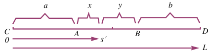
Figure 1: Hotelling duopoly on a one-dimensional line market. Firm $A$ is located at distance $a$ from the left side and firm $B$ is located at distance $b$ from right side. Consumers located in $s\leq s^{\prime}$ would choose firm $A$ and located in $s\geq s^{\prime}$ would choose firm $B$. $x=|s^{\prime}-a|$, $y=|L-b-s^{\prime}|$.

Since

$$\left\{\begin{array}[]{l}p_{1}+t\cdot x=p_{2}+t\cdot y\\ a+x+y+b=L\end{array}\right.,$$ (2)

we can easily get

$$x=\frac{1}{2}\cdot(L-a-b-\frac{p_{1}-p_{2}}{t}),$$ (3)

$$y=\frac{1}{2}\cdot(L-a-b+\frac{p_{1}-p_{2}}{t}).$$ (4)

Substitute the above results into Eq. (1), we have

$$u_{1}=\frac{1}{2}\cdot(L-a-b)\cdot p_{1}-\frac{p_{1}^{2}}{2t}+\frac{p_{1}\cdot p_{2}}{2t},$$ (5)

$$u_{2}=\frac{1}{2}\cdot(L-a-b)\cdot p_{2}-\frac{p_{2}^{2}}{2t}+\frac{p_{1}\cdot p_{2}}{2t}.$$ (6)

On the second stage, $\partial u_{1}/\partial p_{1}=0,\ \partial u_{2}/\partial p_{2}=0$. NE would be

$$p_{1}=t\cdot(L+\frac{a-b}{3}),$$ (7)

$$p_{2}=t\cdot(L-\frac{a-b}{3}).$$ (8)

Thus,

$$u_{1}=\frac{t}{2}\cdot(L+\frac{a-b}{3})^{2},$$ (9)

$$u_{2}=\frac{t}{2}\cdot(L-\frac{a-b}{3})^{2}.$$ (10)

On the first stage, we can easily found out $\partial u_{1}/\partial a>0,\ \partial u_{2}/\partial b>0$. This means that firm $A$ or $B$ would improve its profit when it moves nearer toward each other. With the restriction $0\leq a,b\leq L/2$, the NE solution would actually be $a=L/2,b=L/2.$

This outcome is not satisfactory. If the firms could cooperate and both choose $a=b=L/4$, they would make no less profit, with the transport expense minimized for consumers.

3 Simplified version of $D=1-t\cdot|s-s^{\prime}|$ Hotelling model

3.1 Classical situation

Here we present the classical model we want to quantize in this paper, which is a bit different from the original model. In this model, firstly, we set $D=1-t\cdot|s-s^{\prime}|$, where $s^{\prime}=a$ or $L-b$ is used to index the location of the firm while $s$ is used to index consumer’s location. This ’density demand function’ means consumer is sensitive to the transport cost, but not sensitive to the price of the product, which reveals the fact that even the consumer’s demand is inelastic to the price of the products, it would reduce if the transportation cost becomes high since it is indeed an extra pay added to the original price. Based on this ’density demand function’, we have

$$q_{1}=\int_{0}^{a+x}(1-t\cdot|s-s^{\prime}|)ds=a+x-1/2\cdot t\cdot(a^{2}+x^{2}),$$ (11)

$$q_{2}=\int_{a+x}^{L}(1-t\cdot|s-s^{\prime}|)ds=b+y-1/2\cdot t\cdot(b^{2}+y^{2}).$$ (12)

Secondly, we assume the price of the product for the two firms is determined by the supplier and $p_{1}=p_{2}=p_{0}$. This is often the case if the two ”firms” are in fact two retailers and the retail price of the products has been fixed to a ”unified price” by a powerful manufacture. As a result, $A$ and $B$ would only compete on the location choice with fixed price, and the two-stage Hotelling model was simplified to a one-stage game.

From the first formula of Eq. (2), it is straightly $x=y=\frac{1}{2}\cdot(L-a-b)$. Then the profit functions turn to be

$$u_{1}=p_{0}\cdot[a+\frac{1}{2}(L-a-b)-\frac{1}{2}t(a^{2}+\frac{1}{4}(L-a-b)^{2})],$$ (13)

$$u_{2}=p_{0}\cdot[b+\frac{1}{2}(L-a-b)-\frac{1}{2}t(b^{2}+\frac{1}{4}(L-a-b)^{2})].$$ (14)

For this model, noticing that $0\leq a,b\leq L/2$, three cases of NE can be obtained as follows:

(1) if $t\in[0,1/L)$, then $\partial u_{1}/\partial a>0,\partial u_{2}/\partial b>0$, NE would be $a=b=L/2$. Accordingly, $u_{1}=u_{2}=p_{0}(L/2-L^{2}t/8)$.

(2) if $t\in[1/L,2/L]$, the NE require

$$\partial u_{1}/\partial a=p_{0}\cdot[\frac{1}{2}-\frac{t}{2}\cdot(2a+\frac{a+b-L}{2})]=0,$$ (15)

$$\partial u_{2}/\partial b=p_{0}\cdot[\frac{1}{2}-\frac{t}{2}\cdot(2b+\frac{a+b-L}{2})]=0,$$ (16)

which lead to $a=b=\frac{2+Lt}{6t}\in[L/3,L/2]$, and consequently

$$u_{1}=u_{2}=-p_{0}t[(\frac{2+Lt}{6t}-\frac{L}{4})^{2}+\frac{L^{2}}{16}]+p_{0}\frac{L}{2}.$$ (17)

(3) if $t>2/L$, $t$ is out of reasonable range, since $D=1-t\cdot|s-s^{\prime}|$ is possibly negative.

It can be easily verified that neither of the profits of case (1) or (2) are Pareto efficient. Actually if they cooperated and chose locations as $a=b=L/4$, they could both make higher profits.

3.2 Quantum situation

Now we apply Li’s method Li to quantize the above Hotelling model. In classical game, the strategies of the two firms is directly determined by their independent choice of $a$ and $b$. As a comparison, in quantum game the strategies of the two firms are determined by their independent choice of two quantum variables $x_{1}$ and $x_{2}$, which have the following relationships with $a$ and $b$:

$$a=x_{1}\cosh\gamma+x_{2}\sinh\gamma,$$ (18)

$$b=x_{2}\cosh\gamma+x_{1}\sinh\gamma.$$ (19)

Substituting the above relations into Eq. (13) and (14), we have

$$u_{1} = p_{0}\cdot[(x_{1}\cosh\gamma+x_{2}\sinh\gamma)+\frac{t}{2}(L-x_{1}e^{\gamma}-x_{2}e^{\gamma})$$ (20)

$$-\frac{t}{2}(x_{1}\cosh\gamma+x_{2}\sinh\gamma)^{2}-\frac{t}{2}(L-x_{1}e^{\gamma}-x_{2}e^{\gamma})^{2}],$$

$$u_{2} = p_{0}\cdot[(x_{2}\cosh\gamma+x_{1}\sinh\gamma)+\frac{t}{2}(L-x_{1}e^{\gamma}-x_{2}e^{\gamma})$$ (21)

$$-\frac{t}{2}(x_{2}\cosh\gamma+x_{1}\sinh\gamma)^{2}-\frac{t}{2}(L-x_{1}e^{\gamma}-x_{2}e^{\gamma})^{2}].$$

Similarly to the classical model, the results of the game are classified by the range of $t$:

(1)If $t\in[0,(1-\tanh\gamma)/L)$, we have $\partial u_{i}/\partial x_{i}>0$, NE would be $a=b=L/2$, and $u_{1}=u_{2}=p_{0}(L/2-L^{2}t/8)$ .

When $\gamma=0$, this interval of $t$ would be $[0,1/L)$, which corresponds the classical situation.

When $\gamma\to\infty$, this interval of $t$ would reduce to zero, it means the classical result won’t appear at maximal entanglement.

(2) If $t\in[(1-\tanh\gamma)/L,2/L]$, $\partial u_{i}/\partial x_{i}=0$ has a solution

$$x_{1}=x_{2}=\frac{2\cosh\gamma+Lt\cosh\gamma-2\sinh\gamma+Lt\sinh\gamma}{2t(1+2\cosh 2\gamma+2\sinh 2\gamma)},$$ (22)

and consequently

$$a=b=\frac{2\cosh\gamma+Lt\cosh\gamma-2\sinh\gamma+Lt\sinh\gamma}{6t\cosh\gamma+2t\sinh\gamma}.$$ (23)

When $\gamma=0$, the interval of $t$ would be $[1/L,2/L]$, which is the same as the classical situation.

When $\gamma\to\infty$, the interval of $t$ would expand to $(0,2/L]$, the whole reasonable region except for point $0$, and the NE solution is $a=b=L/4$.

(3) If $t>2/L$, $t$ is out of reasonable range, as we have discussed in 3-1.

Now we check out the quantum profit. We are able to calculate the total quantum profit using the above NE solutions. Here we just present one firm’s profit since the other’s is just the same.

$$u_{iq}=\left\{\begin{array}[]{l@{\quad\ \quad}l}(\frac{L}{2}-\frac{1}{8}L^{2}t)&0\leq t<\frac{1-\tanh\gamma}{L}\\ {\scriptstyle p_{0}t[-(\frac{2\cosh\gamma+Lt\cosh r-2\sinh\gamma+Lt\sinh r}{6t\cosh\gamma+2t\sinh\gamma}-\frac{L}{4})^{2}-\frac{L^{2}}{16}]+p_{0}\frac{L}{2}}&\frac{1-\tanh\gamma}{L}\leq t\leq\frac{2}{L}\end{array}\right.$$ (24)

In 3-1, we have already got the profit for each firms in the classical game, which is listed compactly as follows:

$$u_{ic}=\left\{\begin{array}[]{l@{\quad\ \quad}l}p_{0}(\frac{L}{2}-\frac{1}{8}L^{2}t)&0\leq t<\frac{1}{L}\\ p_{0}t[-(\frac{2+Lt}{6t}-\frac{L}{4})^{2}-\frac{L^{2}}{16}]+p_{0}\frac{L}{2}&\frac{1}{L}\leq t\leq\frac{2}{L}\end{array}\right.$$ (25)

Here, the whole interval of $t$, $[0,2/L]$ could be divided into three regions. In the first region, $0\leq t<\frac{1-\tanh\gamma}{L}$, the profit of quantum game is the same as classical game, and is independent of $\gamma$. In the second region $(1-\tanh\gamma)/L\leq t<1/L$ and the third region $1/L\leq t<2/L$, the quantum prifits are different from the classical ones.

In the second region, $(1-\tanh\gamma)/L\leq t<1/L$,

$$u_{iq}-u_{ic}=\frac{p_{0}(2+e^{2\gamma}Lt)[-2+(1+e^{2\gamma})Lt]}{4(1+2e^{2\gamma})^{2}t}.$$ (26)

Figure 2 is the relation curve of quantum profit of one firm and $\gamma$, and Fig. 3 is the difference between quantum and classical profit (As a comparison, the first region is also plotted in the two figures), which indicate that the quantum profit is more and more exceed the classical one when $\gamma$ increases, and the maximum difference is achieved when $\gamma\to\infty$.

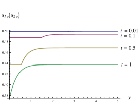
Figure 2: Quantum profit for $0\leq t<1/L$, which includes the first region $0\leq t<\frac{1-\tanh\gamma}{L}$ (where the curve is degenerated into horizonal line) and the second region $(1-\tanh\gamma)/L\leq t<1/L$. Here we set $p_{0}=1,L=1.$

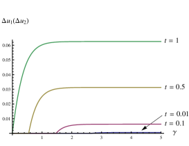
Figure 3: Difference between Quantum and Classical situation, for $0\leq t<1/L$, which includes the first region $0\leq t<\frac{1-\tanh\gamma}{L}$ and the second region $(1-\tanh\gamma)/L\leq t<1/L$. Here we set $p_{0}=1,L=1.$

In the third region, $1/L\leq t\leq 2/L$, similar analysis leads to

$$u_{iq}-u_{ic}=p_{0}t[-\frac{(-4+Lt)^{2}}{16(t+2e^{2\gamma}t)^{2}}+(\frac{L}{4}-\frac{2+Lt}{6t})^{2}].$$ (27)

Figure 4 is the relation curve of quantum profit of one firm and $\gamma$, and Fig. 5 is the difference between quantum and classical profit, which indicate the similar pattern as in the second region, i.e. the quantum advantage becomes more evident when $\gamma$ increases.

It is remarkable that when $\gamma\to\infty$, the quantum profit arrives at Pareto optimum. In addition to this, the consumers’ average travel distance is minimized as $L/8$, only a half value of the classical case.

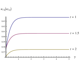
Figure 4: Quantum profit for $1/L\leq t\leq 2/L$. When $\gamma=0$, it turns back to the classical profit. Here we set $p_{0}=1,L=1.$

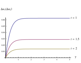
Figure 5: Difference between quantum and classical situation for $1/L\leq t\leq 2/L$. Here we set $p_{0}=1,L=1.$

It is not meaningless to discuss the effect of $t$ on the quantum results. From Fig. 3 and Fig. 5, we can see that the improvement of profit by quantum scheme increases as $t$ increases up to 1; then the improvement decreases with the increasing $t$ if $t>1$. At least such phenomenon shows the complicated coupling effects of the quantization and the travel cost.

4 Full version of $D=1-t\cdot|s-s^{\prime}|$ Hotelling model

4.1 Classical situation

Now we extend the model in section 3 to a more general form. We abandon the restriction of $p_{1}=p_{2}=p_{0}$, and assume the two firms are free to choose their prices. This two-stage model could actually be regarded as a full version of the Hotelling model in section 3.

In this full version of $D=1-t\cdot|s-s^{\prime}|$ Hotelling model, we have

$$u_{1}=p_{1}\cdot[a+\frac{1}{2}(\frac{p_{2}-p_{1}}{t}+L-a-b)-\frac{1}{2}t(a^{2}+\frac{1}{4}(\frac{p_{2}-p_{1}}{t}+L-a-b)^{2})],$$ (28)

$$u_{2}=p_{2}\cdot[b+\frac{1}{2}(\frac{p_{1}-p_{2}}{t}+L-a-b)-\frac{1}{2}t(b^{2}+\frac{1}{4}(\frac{p_{1}-p_{2}}{t}+L-a-b)^{2})].$$ (29)

To solve the equilibrium for this model, we follow the procedure introduced in section 2: first we solve NE of the second stage, then we determine the NE for the first stage. For the second stage, NE requires $\partial u_{1}/\partial p_{1}=0$, $\partial u_{2}/\partial p_{2}=0$, and thus we can get the relation of $p_{1}$, $p_{2}$ and $a$, $b$. Then for the first stage, NE requires $\partial u_{1}/\partial a=0$, $\partial u_{2}/\partial b=0$, from which we can solve the locations, and consequently the prices.

However, the calculation is very complicated. Here we restricted to the symmetric solutions, i.e. we only look for the solutions satisfying $a=b,p_{1}=p_{2}$. The calculation can be much simplified with these restrictions.

$\gamma=0$ in Fig. 6 shows the symmetric solution of the location we found in the classical games. Here we only analysis the situation when $0\leq t\leq 1/L$ rather than $0\leq t\leq 2/L$ when in section 3. This is due to the fact that the prices of the products is variables now, and the restriction $0\leq t\leq 1/L$ is to make sure that $D$ in this case is positive even if the two firms choose largely different prices.

4.2 Quantum situation

For the quantum situation, we use the same scheme as in subsection 3.2, i.e. quantizing the location strategy while keeping the price strategy classical. For the quantum strategy indexed by $x_{1}$ and $x_{2}$, we have relationships (18), (19) presented in subsection 3.2. The profit function $u_{1}$ and $u_{2}$ would be derived using the relationships (28), (29). And for the first stage, we need to investigate the property of $\partial u_{1}/\partial x_{1}$ and $\partial u_{2}/\partial x_{2}.$

The quantum ($\gamma=\mbox{sinh}^{-1}3/4$, and $\gamma\to\infty$) and classical ($\gamma=0$) results of the location of the firms are presented in Fig. 6. And Fig. 7 is the quantum and classical profit of these cases, which indicates the tendency that the quantum game gets a better profit for both firms when $\gamma$ increases.

Figure 6: Classical ($\gamma=0$) and quantum ($\gamma=\sinh^{-1}3/4$ and $\gamma\to\infty$) position for firm $A$ and $B$ as a function of transport cost $t$. Here we set $L=1$.

Figure 7: Classical ($\gamma=0$) and quantum ($\gamma=\sinh^{-1}3/4$ and $\gamma\to\infty$) profit for firm $A$ and $B$ as a function of transport cost $t$. Here we set $L=1$.

The explicit form of the solutions is generally too complicated to write down here, just as in the classical game. But luckily for $\gamma\to\infty$, the solution is simple enough as follows.

$$a=b=\frac{-8+5Lt+\sqrt{64-56Lt+7L^{2}t^{2}}}{12t},$$ (30)

and

$$u_{1}=u_{2}=\frac{{\scriptstyle[5L^{2}t^{2}+Lt(-40+\sqrt{64-56Lt+7L^{2}t^{2}})-4(-8+\sqrt{64-56Lt+7L^{2}t^{2}})]^{2}}}{{\scriptstyle 54t(4-Lt+\sqrt{64-56Lt+7L^{2}t^{2}})}}.$$ (31)

This is the best profit the two firms could make using our quantization scheme.

To better understand the result, let us review the classical game. In the classical game, if the two firms choose locations in such a way that $a=b$, and yet compete in the price choice, the profit could finally be write as

$$u_{1}=u_{2}=\frac{t[8a^{2}t+L(-4-4at+Lt)]^{2}}{16(2+2at-Lt)}.$$ (32)

This function is maximized and turned to be (31) when $a$ and $b$ satisfy (30). This is to say, if the two firms could cooperate in the location stage, they can choose their locations according to (30) to make the best profit for both of them. Thus the maximal entangled quantum scheme does help to realize the best profit, which is impossible in the classical uncooperative game.

5 Conclusion

In this paper, we quantized the first stage of Hotelling model, e.g, the location choice stage, to study the quantum properties of the game. First we present our version of the model and investigated the quantum consequences of the game. The quantum game gave higher profit for both players. And we showed that with $\gamma$ increasing, the quantum benefit over the classical increases too. Then we extended the model to a more general form and we found again, the quantum profit is higher than the classical one. And there is a common tendency that as $\gamma$ increasing, the quantum advantage becomes more evident.

- (1) C. H. Bennett, G. Brassard, C. Cr peau, R. Jozsa, A. Peres, W. K. Wootters, Teleporting an unknown quantum state via dual classical and Einstein-Podolsky-Rosen channels, Phys. Rev. Lett. 70, 1895 (1993)
- (2) D. A. Meyer, Quantum strategies, Phys. Rev. Lett. 82, 1052 (1999)
- (3) J. Eisert, M. Wilkens, M. Lewenstein, Quantum games and quantum strategies, Phys. Rev. Lett. 83, 3077 (1999)
- (4) L. Goldenberg, L.Vaidman, S.Wiesner, Quantum gambling, Phys. Rev. Lett. 82, 3356 (1999)
- (5) S. C. Benjamin, P. M. Hayden, Multiplayer quantum games, Phys. Rev. A 64, 030301 (2001)
- (6) A. Iqbal, A.H. Toor, Quantum repeated games, Phys. Lett. A 300, 541 (2002)
- (7) H. Li, J. Du, S. Massar, Continuous-variable quantum games, Phys. Lett. A 306, 73 (2002)
- (8) C. F. Lo, D. Kiang, Quantum Bertrand duopoly with differentiated products, Phys. Lett. A 321, 94 (2004)
- (9) C. F. Lo, D. Kiang, Quantum stackelberg duopoly, Phys. Lett. A 318, 333 (2003)
- (10) J. Du, H. Li, C. Ju, Quantum games of asymmetric information, Phys. Rev. E. 68, 016124 (2003)
- (11) G. Qin, X. Chen, M. Sun, J. Du, Quantum Bertrand duopoly of incomplete information, J. Phys. A: Math. Gen. 38, 4247 (2005)
- (12) C. F. Lo, D. Kiang, Quantum Stackelberg duopoly with incomplete information, Phys. Lett. A 346, 65 (2005)
- (13) G. Qin, X. Chen, M. Sun, X.Y. Zhou, J. Du, Appropriate quantization of asymmetric games with continuous strategies, Phys. Lett. A 340, 78 (2005)
- (14) H. Hotelling, Stability in competition, Econ. J. 39, 41 (1929)
- (15) For a review, see S. Martin, Advanced Industrial Economics, 2nd ed., Wiley-Blackwell (2001)
- (16) For a recently new form of this model, see Y. M. Chen, M. H. Riordan, Price and variety in the spokes model, Econ. J. 117, 897 (2007)
- (17) R. Rahaman, P. Majumdar, B. Basu, Quantum Cournot equilibrium for the Hotelling CSmithies model of product choice, J. Phys. A: Math. Theor. 45, 455301 (2012)
- (18) See, for example, D. Fudenberg, J. Tirole, Game Theory, MIT Press, Cambridge, MA (1991);R. Gibbons, Game Theory for Applied Economists, Princeton University Press (1992)