Asymptotically Optimum Perfect Universal
Steganography of Finite Memoryless Sources

Abstract

A solution to the problem of asymptotically optimum perfect universal steganography of finite memoryless sources with a passive warden is provided, which is then extended to contemplate a distortion constraint. The solution rests on the fact that Slepian’s Variant I permutation coding implements first-order perfect universal steganography of finite host signals with optimum embedding rate. The duality between perfect universal steganography with asymptotically optimum embedding rate and lossless universal source coding with asymptotically optimum compression rate is evinced in practice by showing that permutation coding can be implemented by means of adaptive arithmetic coding. Next, a distortion constraint between the host signal and the information-carrying signal is considered. Such a constraint is essential whenever real-world host signals with memory (e.g., images, audio, or video) are decorrelated to conform to the memoryless assumption. The constrained version of the problem requires trading off embedding rate and distortion. Partitioned permutation coding is shown to be a practical way to implement this trade-off, performing close to an unattainable upper bound on the rate-distortion function of the problem.

I Introduction

Digital data hiding refers to coding techniques which aim at embedding information within digital discrete-time host signals [1]. In short, steganography is a special data hiding scenario in which undetectability of the embedded information is paramount —unobtrusiveness, rather than undetectability, suffices in general data hiding. In the steganographic problem, a “man in the middle” (warden) performs a detection test on signals sent between two parties in order to determine whether they carry hidden information or not. In the scenario considered here, the warden does not alter the tested signals, which thus arrive unmodified at the decoder (passive warden). Besides circumventing detection by the warden, the encoder also wishes to maximize the steganographic embedding rate, which is the amount of bits per host element that can be conveyed to the decoder through the covert channel created by modifying the host in order to embed (hide) information.

An important landmark in steganography research was the realization of the existence of an inextricable connection between steganography and source coding. Anderson and Petitcolas gave an intuitive rationale for this link in the early days of digital steganography [2, Section VI-A]. These authors pointed out that if we would have lossless source coding with optimum compression rate for real-world signals (i.e., ideal compression for signals such as digital images), then these signals would have to be dense in the space of the optimum source code. Thus, decompressing any arbitrary sequence from this space would always render a true real-world signal. In other words, a lossless compression algorithm with optimum compression rate could also work as a perfect (undetectable) steganographic algorithm with optimum embedding rate, by using decompression to encode a message into an information-carrying signal and compression to decode that message.

This duality between perfect steganography with a passive warden and lossless source coding implied that practical steganographic algorithms had to be intimately related to practical compression algorithms. Soon, some authors partially succeeded in translating this fundamental relationship into well-founded steganographic methods. The first proposal along these lines was in the early work of Cachin [3]. Later on, Sallee added another important piece to the puzzle with model-based steganography [4]. Subsequent research has gradually drifted away from these seminal contributions, and steganography has become a subject for the most part disconnected from source coding. Machine learning has grown in importance, and relevant information-theoretical results such as [5] or [6] have been largely sidelined.

Here we present a contribution which we believe fills an important gap in the field: the asymptotically optimum solution to the canonical steganography problem dual of universal lossless compression of memoryless signals with optimum compression rate. Furthermore, we consider the implications of the application of this solution to real-world signals such as multimedia, and we show its connections with existing results about steganographic systems. The roots of the questions considered here are found in Cachin’s criterion [3]. This criterion tells us that a perfect steganographic system is implemented by an encoder that exactly preserves the distribution of the host signal, because in this way optimum detection by the warden will be foiled. The implementation of Cachin’s criterion raises a crucial issue: what should the encoder do if the distribution of the host signal is not known? As noted by Cachin himself by drawing the parallel with source coding, universal steganography must necessarily be the matter-of-fact approach to implementing perfect steganography: it is the empirical distribution of the host that should be preserved [3]. Thus, a canonical problem in steganography is how to undertake perfect universal steganography of memoryless host signals with optimum embedding rate. The core element of the solution presented here is Slepian’s Variant I permutation coding [7]. The centrality of permutations to the problem at hand was already discovered —either explicitly or not— by a number of researchers over the years, most prominently by Ryabko and Ryabko [8]. However, the answer to the fundamental question is still open: how does one implement a general perfect universal steganographic algorithm for finite memoryless host signals with asymptotically optimum embedding rate?

Cachin’s criterion implicitly assumes that a probabilistic model can completely capture the nature of the signals produced by a steganographic encoder. However this is not generally true whenever real-world signals meaningful to humans (e.g., images, audio, video) are used as hosts, as the semantics of such signals are not accurately captured by any known probabilistic model (in particular by an empirical model on which the universal approach must be based). In the context of this paper semantics become relevant whenever a reversible decorrelating transform is applied to real-world signals with memory, for them to conform to the memoryless assumption [9]. Due to the aforementioned limitations of the models, even if an information-carrying signal can be produced which has the exact statistics of some model, it may still be semantically wrong —and thus suspicious to a human warden. By continuity arguments, enforcing a similarity constraint between host and information-carrying signal —in addition to the empirical statistics preservation constraint— can help preserve the semantics of the host in the information-carrying signal. This constraint implies a second open question: what is the optimum embedding rate for a given similarity constraint (embedding distortion constraint)?

In this paper we address the two questions outlined above. The material is organized as follows. Section II introduces the notational conventions and the basic setting assumed throughout the paper. Section III reviews prior work on steganography of memoryless hosts and motivates our study. Section IV introduces the use of permutation coding for steganography and discusses a low-complexity implementation, which solves the first question. Section V is devoted to a theoretical analysis of the embedding distortion of permutation coding in a steganographic context. Next, Section VI addresses the issue of embedding distortion control and describes a suboptimal solution to the second question. Theoretical and empirical results are compared in Section VII, and, lastly, Section VIII draws the conclusions of this work.

II Preliminaries

Notation

Boldface lowercase Roman letters are column vectors. The $i$-th element of vector $\mathbf{a}$ is $a_{i}$, or $(\mathbf{a})_{i}$ whenever this notation is more convenient. The special symbols $\mathbf{1}$ and $\mathbf{0}$ are the all-ones vector and the null vector, respectively. Capital Greek letters denote matrices; the entry at row $i$ and column $j$ of matrix $\Pi$ is $(\Pi)_{i,j}$. In keeping with standard notation, the only exception to this convention is the exchange matrix $\mathrm{J}$. $\mathrm{I}$ is the identity matrix. $\mathop{\rm tr}\Pi$ is the trace of $\Pi$. $(\cdot)^{t}$ is the transpose operator. $\mathop{\rm diag}(\mathbf{a})$ is a diagonal matrix with $\mathbf{a}$ in its diagonal. The indicator function is defined as $\mathbbold{1}_{\{\theta\}}=1$ if logical expression $\theta$ is true, and zero otherwise. The 2-norm of a vector $\mathbf{r}$ is $\|\mathbf{r}\|=\sqrt{\mathbf{r}^{t}\mathbf{r}}$. The Hamming distance between two $n$-vectors $\mathbf{r}$ and $\mathbf{s}$ is $\delta(\mathbf{r},\mathbf{s})=\sum_{i=1}^{n}\mathbbold{1}_{\{r_{i}\neq s_{i}\}}$. The Hamming weight of $\mathbf{r}$ is $\omega(\mathbf{r})=\delta(\mathbf{r},\mathbf{0})$. Calligraphic letters are sets; $|\mathcal{V}|$ is the cardinality of set $\mathcal{V}$. When describing algorithms, $x\leftarrow v$ means the assignment of value $v$ to variable $x$.

A host sequence is denoted by the discrete-valued $n$-vector $\mathbf{x}=[x_{1},x_{2},\ldots,x_{n}]^{t}\in\mathcal{V}^{n}$ where $\mathcal{V}=\{v_{1},v_{2},\ldots,v_{q}\}\subset\mathbb{Z}$. We assume that $\mathbf{x}\neq\mathbf{0}$, and that $\mathbf{v}=[v_{1},v_{2},\ldots,v_{q}]^{t}$ gives the elements of $\mathcal{V}$ in increasing order, that is, $v_{1}<v_{2}<\cdots<v_{q}$. The histogram of $\mathbf{x}$ is a vector $\mathbf{h}=[h_{1},h_{2},\ldots,h_{q}]^{t}$ such that $h_{k}=\sum_{i=1}^{n}\mathbbold{1}_{\{v_{k}=x_{i}\}}$ for $k=1,2,\ldots,q$, and therefore $\mathbf{h}^{t}\mathbf{1}=n$; $\mathbf{v}$ is hence the vector containing the ordered histogram bins. An information-carrying sequence is denoted by $\mathbf{y}=[y_{1},y_{2},\ldots,y_{n}]^{t}$.

Let $\mathcal{S}_{n}$ be the symmetric group, namely, the group of all permutations of $\{1,2,\ldots,n\}$. We denote a permutation $\boldsymbol{\sigma}\in\mathcal{S}_{n}$ by means of a vector $\boldsymbol{\sigma}=[\sigma_{1},\sigma_{2},\ldots,\sigma_{n}]^{t}$ where $\sigma_{i}\in\{1,2,\ldots,n\}$ and $\sigma_{i}\neq\sigma_{j}$ for all $i\neq j$. This vector defines in turn a permutation matrix ${\Pi}_{\boldsymbol{\sigma}}$ with entries $(\Pi_{\boldsymbol{\sigma}})_{i,j}=\mathbbold{1}_{\{\sigma_{i}=j\}}$. The reordering of $\mathbf{x}$ using $\boldsymbol{\sigma}$ is the vector $\mathbf{y}={\Pi}_{\boldsymbol{\sigma}}\,\mathbf{x}$, for which $y_{i}=x_{\sigma_{i}}$ for $i=1,2,\ldots,n$. Two or more different permutations may lead to the same reordering of the elements of $\mathbf{x}$. For this reason we will follow the convention that a rearrangement of $\mathbf{x}$ is a unique ordering of its elements. A special case is the rearrangement of $\mathbf{x}$ in nondecreasing order. This is obtained by means of a permutation ${\boldsymbol{\sigma}}^{\uparrow}$ yielding ${\mathbf{x}^{\uparrow}}=\Pi_{{\boldsymbol{\sigma}}^{\uparrow}}\,\mathbf{x}$ such that ${x}^{\uparrow}_{\!1}\leq{x}^{\uparrow}_{\!2}\leq\cdots\leq{x}^{\uparrow}_{\!n}$. The rearrangement of $\mathbf{x}$ in nonincreasing order can be obtained from ${\mathbf{x}^{\uparrow}}$ as ${\mathbf{x}^{\downarrow}}=\mathrm{J}{\mathbf{x}^{\uparrow}}$, where $\mathrm{J}$ is the exchange matrix —the permutation matrix with entries $(\mathrm{J})_{i,j}=\mathbbold{1}_{\{j=n-i+1\}}$.

Italicized Roman or Greek capital letters represent random variables. The probability mass function (pmf) of a random variable $X$ with support $\mathcal{V}$ is denoted by $p(X=v)$, with $v\in\mathcal{V}$, or simply by $p(v)$ if clear from the context. We will also refer to $\mathbf{p}=[p(X=v_{1}),p(X=v_{2}),\ldots,p(X=v_{q})]^{t}$ as the pmf of $X$, and to $\mathbf{v}$ as its support. The probability of an event $\vartheta$ is denoted by $\Pr\{\vartheta\}$. The expectation, variance, and entropy of $X$ are denoted by $\mathop{\textrm{E}}\{X\}$, $\mathop{\textrm{Var}}\{X\}$, and $H(X)$, respectively. The binary entropy function is denoted by $h(p)$. $I(X;Y)$ is the mutual information between $X$ and $Y$. Logarithms are base 2 throughout the paper, unless explicitly noted otherwise. Asymptotic equalities and inequalities (as $n\to\infty$) are marked with a dot on top of the usual sign.

Figure 1: Setting studied in the paper: the encoder modifies a host signal $\mathbf{x}$ to produce a signal $\mathbf{y}$ carrying message $m$. Encoder and decoder may share a symmetric secret key $k$. Further parameters are shared in the special case in which a constraint on the embedding distortion $s(\mathbf{x},\mathbf{y})$ is enforced (see Section VI).

Setting

The setting studied in this paper is shown in Figure 1. The encoder is a function $e(\cdot,\cdot):\mathcal{V}^{n}\times\{1,2,\ldots,r\}\to\mathcal{V}^{n}$ which produces an information-carrying signal $\mathbf{y}^{(m)}=e(\mathbf{x},m)$, where $\mathbf{x}$ is the host and $m\in\{1,2,\ldots,r\}$ is the message to be hidden. An alternative view of the encoder is seeing it as adding a watermark $\mathbf{w}^{(m)}\triangleq\mathbf{y}^{(m)}-\mathbf{x}$ to the host $\mathbf{x}$ when it wishes to embed message $m$ in it. In the remainder we will drop the superindex $(m)$ whenever there is no ambiguity, for clarity of exposition. The decoder is a function $d(\cdot):\mathcal{V}^{n}\to\{1,2,\ldots,r\}$ that retrieves the message hidden in a received vector. The decoded message can be put as $\hat{m}=d\left(\mathbf{y}\right)$, and with a passive warden $d\left(\mathbf{y}^{(m)}\right)=m$. The embedding rate (transmission rate) is defined as $\rho\triangleq(1/n)\log r$ (bits/host element). The closeness or similarity between $\mathbf{x}$ and $\mathbf{y}$ is gauged through a function $s(\cdot,\cdot):\mathcal{V}^{n}\times\mathcal{V}^{n}\to[0,\infty)$ such as those discussed in Sections V-A and V-B; $s(\mathbf{x},\mathbf{y}^{(m)})$ can be seen as measuring the embedding distortion caused by hiding message $m$ in $\mathbf{x}$.

We will assume that $\mathbf{x}$ is drawn from a discrete memoryless source. As discussed in Section III, achieving perfect steganography in these conditions requires that $\mathbf{y}$ and $\mathbf{x}$ always have identical empirical distribution (histogram). The fundamental goal is the maximization of the embedding rate $\rho$ under this constraint. As we have mentioned, we will also study the maximization of $\rho$ under a constraint on $s(\mathbf{x},\mathbf{y})$.

As shown in Figure 1, the encoding and decoding functions can also depend on a symmetric secret key for privacy, that is, $e_{k}(\cdot,\cdot)$ and $d_{k}(\cdot)$. For simplicity, and without loss of generality, we will omit this key from most of our exposition, although we will show how to implement keyed encoding/decoding.

III Prior Work and Problem History

Cachin was the first to sketch an answer to the problem of maximum rate steganography of memoryless signals, relying on a description of a generic universal compressor based on the method of types [3]. The construct proposed by Cachin suffers from two shortcomings: 1) it does not provide perfect steganography for finite hosts, as it only achieves perfection asymptotically when the size of the host goes to infinity; 2) it assumes that all signals with the same empirical distribution as the host are valid outputs of the encoder. The first shortcoming was addressed by Ryabko and Ryabko [8], who described a universal steganographic algorithm with optimum embedding rate for finite hosts. Apart from not providing a completely general implementation, the authors of [8] do not address the second shortcoming —the most acute in practical scenarios as we argue next. Recalling the duality argument by Anderson and Petitcolas in the introduction, observe that, in their idealized setting, the encoder produces an information-carrying signal ab initio, relying on an ideal model of the signals that the encoder can output and without the need for a host signal. Yet, in a universal approach, such as in [3] or in [8], the role of the hypothetical ideal host model is played by the empirical model of a given host. A key observation to be made is: nothing guarantees that all signals which preserve the empirical model of the host will also be “close” to it. This is critical when decorrelation of real-world signals with memory is used to conform to the memoryless assumption [9]: not all signals that preserve the first-order statistics of a host signal in the decorrelated domain will map back to semantically meaningful real-world signals in the original domain. As we have discussed, this issue can be remediated by enforcing a similarity constraint between host and information-carrying signal (embedding distortion constraint). This constraint implies that practical steganography must be a problem of coding with noncausal side information at the encoder [10], where the host $\mathbf{x}$ constitutes the deterministic side information.

In regard to the embedding distortion constraint, a practical approach to the problem of near-perfect steganography of finite memoryless sources with asymptotically optimum embedding rate was given by Sallee [4]. This author used the quantized block discrete cosine transform (DCT) domain as a rough approximation to a domain where the host is memoryless, and in which theoretical probabilistic models are available (the generalized Cauchy distribution is used in [4]). Exploiting these two properties Sallee proposed a scheme called model-based steganography which uses arithmetic coding to achieve asymptotically optimum embedding rate while preserving a first-order model of the host, simultaneously constraining the embedding distortion. However, its reliance on a theoretical model of the host means that model-based steganography is neither universal nor perfect.

For a memoryless host signal, perfect universal steganography is achieved by preserving its first-order statistics. If the host is finite and discrete-valued, preserving its first-order statistics is equivalent to preserving its histogram. A number of previous authors more or less explicitly claim that their steganographic algorithms implement histogram preservation. However, on close examination, many allegedly histogram-preserving methods are only approximations. We will briefly review next the few methods that do implement exact histogram preservation, which therefore implement perfect steganography of finite memoryless sources. Among them we find Provos’ OutGuess [11] —the first histogram-preserving steganographic algorithm—, Franz’s proposal [12], Ryabko and Ryabko’s method [8], Kumar and Newman’s J3 [13], and Luo and Subbalakshmi’s method [14].

Most of these methods (see [11, 12, 13]) are variations of least-significant bit (LSB) steganography. In this early heuristic steganographic method the encoder embeds a message into a host $\mathbf{x}$ by producing a signal $\mathbf{y}$ whose elements are $y_{i}=2\lfloor x_{i}/2\rfloor+b_{i}$ for $i=1,2,\ldots,n$, where $b_{i}\in\{0,1\}$ is the message bit embedded in the $i$-th element of the host. The histogram-preserving methods in [11, 12] and [13] can be seen as using LSB steganography plus some kind of histogram compensation to remediate the lack of histogram preservation in the baseline technique. These beginnings limit their possibilities. For instance, all of the methods just cited possess a low embedding rate. The report in [11] suggests that the average embedding rate of Outguess lies around 0.31 bits/host element, whereas Franz’s method is below 0.20 bits/host element for most of the hosts tested in [12], and J3 offers rates between 0.35 bits/host element and 0.65 bits/nonzero host element [13], all clearly below the ceiling embedding rate of 1 bit/host element implemented by LSB steganography.

The exception among all histogram-preserving works in terms of generality and embedding rate is the already mentioned proposal by Ryabko and Ryabko [8], which realizes the following fundamental observation: any information-carrying vector $\mathbf{y}$ that preserves the histogram of $\mathbf{x}$ must be a rearrangement of $\mathbf{x}$. This is because histogram preservation implies that $\sum_{i=1}^{n}\mathbbold{1}_{\{v_{k}=y_{i}\}}=\sum_{i=1}^{n}\mathbbold{1}_{\{v_{k}=x_{i}\}}$ for all $k=1,2,\ldots,q$, which can only be true if $\mathbf{y}=\Pi_{\boldsymbol{\sigma}}\,\mathbf{x}$ for some permutation $\boldsymbol{\sigma}\in\mathcal{S}_{n}$. This observation means that the perfect steganographic codes for finite memoryless hosts are the Variant I permutation codes first described by Slepian [7]. This observation was first made by Franz [12], but Ryabko and Ryabko [8] pursued it further in their proposal of asymptotically optimum perfect steganography. However their method relies on the algorithm in [15] for enumerating combinatorial objects with $O((\log n)^{c})$ time complexity, which, although implementable in special cases, has exponential memory requirements in general.

As for other algorithms which are explicitly based on rearrangements, their embedding rate is limited by the fact that they do not exploit the whole spectrum of histogram-preserving possibilities. For instance [14], based on permuting pairs of host elements, can only achieve a maximum rate of 0.5 bits/host element. We must also mention that Mittelholzer [16] was the first to consider Slepian’s permutation modulation as a steganographic tool. However he studied the non-histogram-preserving case $\mathbf{y}=\mathbf{x}+\Pi_{\boldsymbol{\sigma}}\mathbf{k}$, with $\mathbf{k}$ a secret vector, which is not relevant to our problem.

Finally, we outline how previous histogram-preserving approaches have dealt with the embedding distortion issue. Ryabko and Ryabko [8] did not consider any such constraints. Other histogram-preserving methods [11, 12, 13, 14] do implement embedding distortion control but only in ad hoc ways, and so they are not generally amenable to rate-distortion trade-off optimization.

IV Permutation Codes as Steganographic Codes

We firstly explore the implications of taking to its full extent the previous observation about optimum histogram-preserving steganography of finite memoryless sources necessarily involving Slepian’s permutation coding with $\mathbf{x}$ as the base codeword. Observe that the central difference with respect to the use of permutation codes in channel/source coding [7, 17] is that $\mathbf{x}$ is not a design choice here, but a fixed input parameter of the encoder (see Figure 1). As we will see, this fact is at the root of the two most relevant challenges we will deal with: encoder complexity and embedding distortion control.

IV-A Embedding rate

We state next some basic facts and definitions about permutation coding which we will use throughout the paper. The number $r$ of rearrangements of $\mathbf{x}$ only depends on its histogram $\mathbf{h}$, and it is given by the following multinomial coefficient:

$$r\triangleq{n\choose\mathbf{h}}=\frac{n!}{h_{1}!h_{2}!\cdots h_{q}!}.$$ (1)

Hence the $r$ rearrangements $\mathbf{y}^{(1)},\mathbf{y}^{(2)},\ldots,\mathbf{y}^{(r)}$ of the host $\mathbf{x}$ are the only codewords that the encoder can produce. Hereafter we will consider $\mathcal{S}_{\mathbf{x}}\subset\mathcal{S}_{n}$ to be any set of permutations leading to the $r=|\mathcal{S}_{\mathbf{x}}|$ rearrangements of $\mathbf{x}$.

The embedding rate $\rho=(1/n)\log r$ bits/host element associated to the permutation code based on host $\mathbf{x}$ is necessarily optimum for first-order perfect steganography, as its calculation incorporates all possible codewords. In order to obtain a probabilistic perspective of this quantity, assume next that Stirling’s approximation $\log_{e}z!\approx z\log_{e}z-z$ (for large $z$) holds for all factorials in (1). In this case the rate can be informally approximated as

$$\rho\approx-\sum_{k=1}^{q}\frac{h_{k}}{n}\log\frac{h_{k}}{n}\quad\text{bits/host element}.$$

If $X$ is a discrete random variable whose probability mass function is the type of $\mathbf{x}$, $X\sim\mathbf{p}\triangleq(1/n)\mathbf{h}$, then

$$\rho\approx H(X).$$ (2)

This interpretation of the multinomial coefficient in terms of the entropy of the subjacent type has been known since the definition of entropy; in the context of permutation coding it was first mentioned by Berger et al. [17]. More rigorously, approximation (2) is supported by the following bounds (see for instance [18]):

$$H(X)-\zeta^{(q,n)}\leq\rho\leq H(X),$$ (3)

where $\zeta^{(q,n)}\triangleq(q/n)\log(n+1)$, which show that $\rho\to H(X)$ as $n\to\infty$, i.e., $\rho\doteq H(X)$. The upper bound in (3) on the capacity of perfect steganography was previously given by Cachin [3] using the method of types, and by Comesaña and Pérez-González [5] and Wang and Moulin [6] departing from Gel’fand and Pinskers’ capacity formula, whereas Ryabko and Ryabko [8] gave a lower bound alternative to the one in (3).

IV-B Asymptotically optimum encoding algorithm

Even for moderate $n$, the exponentially growing number of rearrangements of $\mathbf{x}$ precludes the implementation of a naive encoding scheme, such as a look-up table mapping messages to rearrangements. Therefore an efficient method to encode messages into rearrangements (unranking) and to decode messages from rearrangements (ranking) is essential for a practical implementation of permutation coding in steganography.

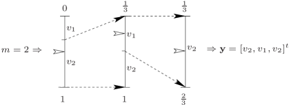
(a) Permutation encoding example

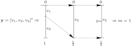
(b) Permutation decoding example

Figure 2: Toy example illustrating the use of adaptive arithmetic coding to undertake permutation encoding and decoding of vectors with histogram $\mathbf{h}=[1,2]^{t}$ and support $\mathbf{v}=[v_{1},v_{2}]^{t}$, for which $r=3$. The three stages depicted represent the right-open intervals $\mathcal{I}^{(0)},\mathcal{I}^{(1)}$, and $\mathcal{I}^{(2)}$. The white arrow gives the position $(m-1/2)/r$ of message $m$ in $[0,1)$.

We will describe next a general encoding procedure which is implementable with $O(n)$ complexity, and which explicitly uses the duality between optimum perfect universal steganography and optimum lossless universal source coding. Consider the lossless compression of a realization $\mathbf{x}$ of a memoryless signal whose statistics $\mathbf{p}$ (or histogram $\mathbf{h}$) are known beforehand. It is well known that, using the static model $\mathbf{h}$ of the counts of the support symbols $\mathbf{v}$ in $\mathbf{x}$, arithmetic coding [19, 20] can compress $\mathbf{x}$ with $O(n)$ complexity to the asymptotic compression rate $H(X)$ (as $n\to\infty$). In a finite context, the compression rate can be improved by adaptively updating the model after each symbol in $\mathbf{x}$ is processed by the arithmetic encoder [21], so as to reflect the updated distribution of the symbols yet to be encoded. In this case the model is initially $\mathbf{h}$, as in the static case, but after a symbol is encoded its corresponding count is decremented by one. This adaptive procedure leads to the implementation of enumerative encoding by means of arithmetic coding. Every sequence $\mathbf{y}$ with the same histogram $\mathbf{h}$ as $\mathbf{x}$, i.e., $\mathbf{y}=\Pi_{\boldsymbol{\sigma}}\mathbf{x}$, is compressed to a sequence that can be seen as the index enumerating $\mathbf{y}$ in the lexicographic ordering established by $\mathbf{v}$. The theoretical equivalence between enumerative coding and arithmetic coding was originally shown by Rissanen [22], and Cleary and Witten demonstrated this equivalence in a constructive way by putting forward the decrementing adaptive model idea sketched above [21].

For the sake of clarity, we will explicitly describe the enumerative encoding scheme before discussing its role in optimum perfect universal steganography. Assume that we wish to compress $\mathbf{y}=\Pi_{\boldsymbol{\sigma}}\mathbf{x}$ using arithmetic coding with the adaptive model discussed above. The initial right-open interval for the arithmetic encoder is $\mathcal{I}^{(0)}\leftarrow[0,1)$, and we also make the initialization $\mathbf{h}^{(0)}\leftarrow\mathbf{h}$. Then the $i$-th arithmetic encoding stage (for $i=1,2,\ldots,n$) comprises the following three steps:

1. Division step: $\mathcal{I}^{(i-1)}$ is exactly divided into nonoverlapping right-open subintervals whose lengths are the nonzero fractions $\mathbf{h}^{(i-1)}/(n-i+1)$ of the length of $\mathcal{I}^{(i-1)}$. Each subinterval for which $h_{k}^{(i-1)}>0$ is labeled with symbol $v_{k}$ from $\mathbf{v}$.

2. Encoding step: the subinterval whose label $v_{s}$ is equal to $y_{i}$ is declared to be the next interval $\mathcal{I}^{(i)}$.

3. Adaptation step: let $h^{(i-1)}_{s}\leftarrow h^{(i-1)}_{s}-1$ and then declare $\mathbf{h}^{(i)}\leftarrow\mathbf{h}^{(i-1)}$.

If we denote the length of $\mathcal{I}^{(i)}$ by $|\mathcal{I}^{(i)}|$ then, for any $\mathbf{y}=\Pi_{\boldsymbol{\sigma}}\mathbf{x}$, it always holds for the final interval that $|\mathcal{I}^{(n)}|=\prod_{i=0}^{n-1}|\mathcal{I}^{(i)}|=1/{n\choose\mathbf{h}}=1/r$. Also, by construction, the final intervals are always nonoverlapping for any two different rearrangements $\mathbf{y}$ of $\mathbf{x}$. Thus the $\lceil\log r\rceil+1$ most significant fractional bits of the binary representation of the midpoint of $\mathcal{I}^{(n)}$ constitute the compressed representation of $\mathbf{y}$ (Shannon-Fano-Elias coding), or its index from the viewpoint of enumerative encoding. This representation can also be put as the most significant $\lceil\log r\rceil+1$ fractional bits of the binary representation of $(m-1/2)/r\in[0,1)$, for some $m\in\{1,2,\ldots,r\}$. Decompressing $\mathbf{y}$ from $m$ requires the same initialization and the same division and adaptation steps as above, whereas the $i$-th decoding step involves declaring the decoded symbol $y_{i}$ to be equal to the symbol $v_{s}$ which labels the subinterval where $(m-1/2)/r$ lies.

We are now ready to outline the permutation coding algorithm, which is simply the dual of the enumerative encoding algorithm just explained. The permutation encoder obtains the rearrangement $\mathbf{y}=e(\mathbf{x},m)$ by carrying out adaptive arithmetic decoding of $m$ as described above. On the other hand, the permutation decoder retrieves the message $m$ embedded in $\mathbf{y}$, that is, $m=d(\mathbf{y})$, by carrying out adaptive arithmetic encoding of $\mathbf{y}$. The decrementing adaptive model guarantees that $\mathbf{y}=\Pi_{\boldsymbol{\sigma}}\mathbf{x}$ for some $\boldsymbol{\sigma}\in\mathcal{S}_{\mathbf{x}}$. Crucially, the permutation encoder and the permutation decoder share $\mathbf{h}$ —the essential piece of information required for encoding and decoding— precisely because of this fact. This is an important difference with respect to the use of enumerative encoding in compression, where the encoder must send the model $\mathbf{h}$ along with the index to the decoder. The permutation encoding and decoding procedures are illustrated in Figure 2.

Some words are in order about the implementability of the algorithm. Since $\lceil\log r\rceil+1>\log r$, the permutation encoder can map some different messages to the same rearrangement, which leads to unsolvable ambiguities at the decoder. Univocal decoding is only guaranteed if at most $\lfloor\log r\rfloor$ bits are used to represent the messages. This is not a serious limitation because (1) is usually very large in steganographic applications, and then $2^{\lfloor\log r\rfloor}\approx r$.

Finally, we would like to remark that the algorithm is closely related to the one proposed by Berger et al. [17, Appendix VI] in the context of the application of permutation codes to source coding with a distortion constraint. Although the complexity of the algorithm in [17] is claimed to be $O(n)$, it is based on Jelinek’s implementation of Shannon-Fano-Elias coding, and therefore the claim can only be true for small $n$ as indicated by Pasco [19, page 11].

Keyed encoding

A way for incorporating a symmetric secret key $k\in\mathcal{K}\subset\mathbb{N}$ into the algorithm above is to use $k$ to select a permutation $\boldsymbol{\varsigma}\in\mathcal{S}_{q}$ to be applied to the vectors $\mathbf{h}$ and $\mathbf{v}$, which are implicitly shared by encoder and decoder. In other words, the algorithm stays the same, but encoder and decoder use $\mathbf{h}^{{\boldsymbol{\varsigma}}}=\Pi_{\boldsymbol{\varsigma}}\mathbf{h}$ and $\mathbf{v}^{{\boldsymbol{\varsigma}}}=\Pi_{\boldsymbol{\varsigma}}\mathbf{v}$ instead of $\mathbf{h}$ and $\mathbf{v}$. With this strategy $|\mathcal{K}|=q!$ because all values in $\mathbf{v}$ are unique, even though this is not true in general for $\mathbf{h}$. If we represent the key using $\lfloor\log q!\rfloor$ bits, then $\mathbf{h}^{\boldsymbol{\varsigma}}$ and $\mathbf{v}^{\boldsymbol{\varsigma}}$ can also be found by means of the permutation coding algorithm that we have described. Finally, $|\mathcal{K}|$ can be increased by choosing $t$ permutations $\boldsymbol{\varsigma}^{(1)},\boldsymbol{\varsigma}^{(2)},\ldots,\boldsymbol{\varsigma}^{(t)}\in\mathcal{S}_{q}$ and then using $\boldsymbol{\varsigma}^{(((i-1)\!\!\mod t)+1)}$ in the $i$-th arithmetic coding stage.

V Embedding Distortion

In this section we will analyze the theoretical embedding distortion induced by permutation coding, and its connections to the embedding rate. For the time being we will not occupy ourselves with the practical question of how to control the embedding distortion. However, as we will see in Section VI, the analysis that follows will be key for a practical implementation of distortion-constrained permutation coding.

V-A Squared Euclidean distance

A useful way to measure the embedding distortion is by means of the squared Euclidean distance between a codeword $\mathbf{y}$ and the host $\mathbf{x}$. In this case the similarity measure in Figure 1 is $s(\mathbf{x},\mathbf{y})=\|\mathbf{y}-\mathbf{x}\|^{2}=\|\mathbf{w}\|^{2}$, which is the squared 2-norm of the watermark. We will also refer to it as the power of $\mathbf{w}$. The main reasons for considering this embedding distortion measure are the following ones: 1) it enables direct comparisons with prior research results when normalized by the power of the host, which yields communications-like signal to noise ratios widely adopted in data hiding (see Section V-A1); 2) it is amenable to analysis and, as it will be seen, it provides relevant insights about the use of permutation coding in steganography, both in terms of geometry and of rate-distortion properties; and 3) if $\mathbf{x}$ is the product of a decorrelating unitary linear transform, then $\|\mathbf{w}\|^{2}$ is preserved in the original (correlated) domain.

Using the fact that all histogram-preserving codewords $\mathbf{y}$ have the same 2-norm $\|\mathbf{y}\|=\|\mathbf{x}\|$, the power of a histogram-preserving watermark can be put as

$$\|\mathbf{w}\|^{2}=2\,(\|\mathbf{x}\|^{2}-\mathbf{x}^{t}\mathbf{y})=2\,(\|\mathbf{x}\|^{2}-\mathbf{x}^{t}\Pi_{\boldsymbol{\sigma}}\mathbf{x})$$ (4)

for some $\boldsymbol{\sigma}\in\mathcal{S}_{\mathbf{x}}$. Since this distortion is dependent on the message associated to $\boldsymbol{\sigma}$, we will derive next two relevant message-independent embedding distortion measures, which will be seen to completely suffice in order to approximate and/or bound (4) for any $\boldsymbol{\sigma}$.

• Average watermark power. If the encoder chooses messages uniformly at random, then the average watermark power is $\overline{\|\mathbf{w}\|^{2}}\triangleq(1/r)\sum_{m=1}^{r}\|\mathbf{w}^{(m)}\|^{2}=2\,\left(\|\mathbf{x}\|^{2}-(1/r)\sum_{\boldsymbol{\sigma}\in\mathcal{S}_{\mathbf{x}}}\mathbf{x}^{t}\ \Pi_{\boldsymbol{\sigma}}\mathbf{x}\right)$. Using next expressions (69) and (70) from the Appendix, and observing that $\mathbf{x}^{t}\mathbf{1}\mathbf{1}^{t}\mathbf{x}=(\mathbf{x}^{t}\mathbf{1})^{2}$, one arrives at

  $$\overline{\|\mathbf{w}\|^{2}}=2\,\left(\|\mathbf{x}\|^{2}-\frac{1}{n}(\mathbf{x}^{t}\mathbf{1})^{2}\right).$$ (5)

  Since $(\mathbf{x}^{t}\mathbf{1})^{2}\geq 0$ it holds that

  $$\overline{\|\mathbf{w}\|^{2}}\leq 2\|\mathbf{x}\|^{2},$$ (6)

  with equality for any zero-sum $\mathbf{x}$. As we will see, the average watermark power plays a pivotal role in the application of permutation coding to steganography. For a start, we verify next that (5) indicates already that permutation coding satisfies fundamental theoretical requirements of perfect steganography. The average watermark power per host element can be put as

  $$\frac{1}{n}\overline{\|\mathbf{w}\|^{2}}=2\;\sigma^{2}_{\mathbf{x}},$$ (7)

  where $\sigma^{2}_{\mathbf{x}}$ is the (biased) sample variance of $\mathbf{x}$. Since the maximum embedding rate is achieved when the encoder is free to generate all rearrangements of $\mathbf{x}$, then (7) is the exact coding analogous of the theoretical result by Comesaña and Pérez-González in [5, page 17] showing that the average quadratic embedding distortion in unconstrained capacity-achieving perfect steganography is

  $$\frac{1}{n}\mathop{\textrm{E}}\{\|\boldsymbol{W}\|^{2}\}=2\mathop{\textrm{Var}}\{X\},$$ (8)

  where $X$ is a random variable describing an independent and identically distributed (i.i.d.) host, and $\boldsymbol{W}$ is a random $n$-vector describing a perfect watermark.

• Maximum watermark power. It is also desirable to obtain the maximum power of a perfect steganographic watermark, $\|\mathbf{w}\|^{2}_{\mathrm{max}}\triangleq\max_{m\in\{1,2,\ldots,r\}}\|\mathbf{w}^{(m)}\|^{2}$, which is the worst-case embedding distortion. To this end we may use the following rearrangement inequality [23, Chapter 10]:

  $${{\mathbf{r}^{\uparrow}}}^{t}{\mathbf{s}^{\downarrow}}\leq\mathbf{r}^{t}\mathbf{s},$$ (9)

  which holds for any $\mathbf{r},\mathbf{s}\in\mathbb{R}^{n}$. Setting $\mathbf{r}=\mathbf{x}$ and $\mathbf{s}=\mathbf{y}$, as $\mathbf{y}=\Pi_{\boldsymbol{\sigma}}\mathbf{x}$ we have from (4) and (9) that

  $$\|\mathbf{w}\|^{2}_{\mathrm{max}}=2\left({\|\mathbf{x}\|^{2}-{\mathbf{x}^{\uparrow}}}^{t}{\mathbf{x}^{\downarrow}}\right).$$ (10)

  An upper bound on $\|\mathbf{w}\|^{2}_{\mathrm{max}}$ is not immediately apparent from inspecting (10), because ${\mathbf{x}^{\uparrow}}^{t}{\mathbf{x}^{\downarrow}}$ may be negative. Since $\mathrm{J}=\mathrm{J}^{t}$, in order to bound $\|\mathbf{w}\|^{2}_{\mathrm{max}}$ from above we can use the Rayleigh-Ritz theorem to write ${\mathbf{x}^{\uparrow}}^{t}{\mathbf{x}^{\downarrow}}={\mathbf{x}^{\uparrow}}^{t}\mathrm{J}{\mathbf{x}^{\uparrow}}\geq\lambda_{\mathrm{min}}(\mathrm{J})\|\mathbf{x}\|^{2}$, where $\lambda_{\mathrm{min}}(\mathrm{J})$ is the minimum eigenvalue of $\mathrm{J}$. By definition, an eigenvalue $\lambda$ of $\mathrm{J}$ and its eigenvector $\mathbf{u}$ fulfill $\mathrm{J}\mathbf{u}=\lambda\mathbf{u}$. Multiplying this expression by $\mathbf{u}^{t}$ one obtains $\mathbf{u}^{t}\mathrm{J}\mathbf{u}=\lambda\|\mathbf{u}\|^{2}$; alternatively, multiplying it by $\mathbf{u}^{t}\mathrm{J}$ one obtains $\|\mathbf{u}\|^{2}=\lambda\mathbf{u}^{t}\mathrm{J}\mathbf{u}$, because $\mathrm{J}$ is involutory ($\mathrm{J}\mathrm{J}=\mathrm{I}$). Combining these two equations one sees that $\lambda^{2}=1$, and since $\mathop{\rm tr}\mathrm{J}\in\{0,1\}$ then $\lambda_{\mathrm{min}}(\mathrm{J})=-1$ when $n>1$. Therefore

  $$\|\mathbf{w}\|^{2}_{\mathrm{max}}\leq 4\|\mathbf{x}\|^{2}.$$ (11)

  As we will see in Section V-A3, this inequality can be more directly obtained through geometric arguments; we will discuss when equality occurs in (11) in that section.

Finally, a basic inequality involving (5) and (10) is

$$\overline{\|\mathbf{w}\|^{2}}\leq\|\mathbf{w}\|^{2}_{\mathrm{max}},$$ (12)

in which equality occurs when $\mathbf{x}=v\mathbf{1}$. In this case $r=1$, and so $\overline{\|\mathbf{w}\|^{2}}=\|\mathbf{w}\|^{2}_{\mathrm{max}}=0$.

V-A1 Power ratios

The embedding distortion expressions (5) and (10) must be normalized in order to be meaningful across different hosts. Thus, the following figures of merit for the theoretical embedding distortion can be put forward:

• Host to average watermark power ratio

  $$\underline{\xi}\triangleq\frac{\|\mathbf{x}\|^{2}}{\overline{\|\mathbf{w}\|^{2}}}.$$ (13)

  A common alternative to $\underline{\xi}$ is the peak host to average watermark power ratio $\underline{\xi}^{\prime}\triangleq n(2^{b}-1)^{2}/\overline{\|\mathbf{w}\|^{2}}$, where it is assumed that $\mathbf{x}$ is in the nonnegative orthant and represented using $b$ bits/element.

• Host to maximum watermark power ratio

  $$\xi_{\mathrm{min}}\triangleq\frac{\|\mathbf{x}\|^{2}}{\|\mathbf{w}\|^{2}_{\mathrm{max}}}.$$

These figures of merit are related as follows:

$$\underline{\xi}^{\prime}\geq\underline{\xi}\geq\xi_{\mathrm{min}}.$$ (14)

In keeping with standard conventions and where convenient throughout the paper, we will also refer to $\xi$ ratios in terms of decibels (dB), by which the amount $10\log_{10}\xi$ is understood. For all the convenience of these figures of merit, a word of caution is needed: as a rule, low $\xi$ ratios imply dissimilarity between $\mathbf{x}$ and $\mathbf{y}$ (or of their counterparts in the original domain if decorrelation is used to approximate the memoryless hypothesis), but the converse is not always true. An example of this shortcoming is the widely used peak signal to noise ratio (PSNR) of which $\underline{\xi}^{\prime}$ is a version. According to our discussion, high $\xi$ ratios are a necessary condition to ensure similarity. However (6) implies that $\underline{\xi}\geq 1/2$ ($\approx-3$ dB), whereas (11) implies that $\xi_{\mathrm{min}}\geq 1/4$ ($\approx-6$ dB). The fact that both minima are very low makes it clear that a mechanism for embedding distortion control will be required whenever similarity must be enforced, which will be dealt with in Section VI.

Finally, our discussion about the analogy between (7) and (8) also let us see why the host to average embedding distortion ratio of capacity-achieving perfect steganography for zero-mean $X$ in [5] coincides with $\underline{\xi}$ for zero-sum $\mathbf{x}$, that is to say, $\underline{\xi}\approx-3$ dB.

V-A2 Asymptotics

We will study next the asymptotic behavior for large $n$ of the power a histogram-preserving watermark drawn uniformly at random, corresponding to the encoder choosing messages uniformly at random. Our aim is to quantify a condition under which (5) is a good predictor of the power of any histogram-preserving watermark, via the weak law of large numbers. In order to do so we will obtain Chebyshev’s inequality for the random variable $\|\boldsymbol{W}\|^{2}=2(\|\mathbf{x}\|^{2}-\mathbf{x}^{t}\mathit{\Pi}\mathbf{x}$), defined using (4) and assuming that $\mathit{\Pi}$ is a random variable uniformly distributed over a set of permutation matrices of cardinality $|\mathcal{S}_{\mathbf{x}}|$ that can generate all rearrangements of $\mathbf{x}$. We know already that $\mathop{\textrm{E}}\{\|\boldsymbol{W}\|^{2}\}=\overline{\|\mathbf{w}\|^{2}}$, and therefore we just need to obtain the second moment of $\|\boldsymbol{W}\|^{2}$ to compute its variance. As $\mathbf{x}^{t}\Pi\mathbf{x}=\mathbf{x}^{t}\Pi^{t}\mathbf{x}$, this moment can be put as

$$\mathop{\textrm{E}}\!\left\{\|\boldsymbol{W}\|^{4}\right\} = 4\,\mathbf{x}^{t}\left(\mathbf{x}\mathbf{x}^{t}-2\|\mathbf{x}\|^{2}\mathop{\textrm{E}}\{\mathit{\Pi}\}+\mathop{\textrm{E}}\!\left\{\mathit{\Pi}\mathbf{x}\mathbf{x}^{t}\mathit{\Pi}^{t}\right\}\right)\mathbf{x},$$

and hence the desired variance is

$$\mathop{\textrm{Var}}\left\{\|\boldsymbol{W}\|^{2}\right\} = 4\left(\mathbf{x}^{t}\mathop{\textrm{E}}\!\left\{\mathit{\Pi}\mathbf{x}\mathbf{x}^{t}\mathit{\Pi}^{t}\right\}\mathbf{x}-\left(\mathbf{x}^{t}\mathop{\textrm{E}}\{\mathit{\Pi}\}\mathbf{x}\right)^{2}\right).$$ (15)

Using the computation of the two expectations in (15) found in the Appendix, it can be seen after some algebraic manipulations that (15) becomes

$$\mathop{\textrm{Var}}\left\{\|\boldsymbol{W}\|^{2}\right\} = \frac{1}{n-1}\left(\overline{\|\mathbf{w}\|^{2}}\right)^{2}.$$

Finally, we use $\mathop{\textrm{Var}}\{\|\boldsymbol{W}\|^{2}\}$ and $\mathop{\textrm{E}}\{\|\boldsymbol{W}\|^{2}\}$ in Chebyshev’s inequality for $\|\boldsymbol{W}\|^{2}$. Given $\gamma>0$, this inequality can be put as $\Pr\{|Z-\mu|\geq\gamma\mu\}\leq\sigma^{2}/(\gamma^{2}\mu^{2})$ for a variable $Z$ with mean $\mu$ and variance $\sigma^{2}$. Thus we obtain

$$\Pr\left\{\left|\|\boldsymbol{W}\|^{2}-\overline{\|\mathbf{w}\|^{2}}\right|\geq\gamma\overline{\|\mathbf{w}\|^{2}}\right\}\leq\frac{1}{\gamma^{2}(n-1)}.$$ (16)

Although Chebyshev’s inequality is known to be loose it is also completely general, and it can be read as saying that the embedding distortion associated to a randomly drawn permutation codeword is not likely to be too different from the average $\overline{\|\mathbf{w}\|^{2}}$ for large $n$. This fact will be empirically verified in Section VII.

Despite these considerations, one might still be concerned about the rare instances in which $\|\boldsymbol{W}\|^{2}$ deviates from the average. We will see next that the geometry of permutation coding strictly confines the maximum distortion (10) in terms of the average distortion (5).

V-A3 Geometry

As noted by Slepian [7], the two basic observations to be made about the geometry of permutation codes are: 1) since $\|\mathbf{y}\|=\|\mathbf{x}\|$, then all codewords lie on an $n$-dimensional primary permutation sphere centered at $\mathbf{0}$ with radius $\|\mathbf{x}\|$; and 2) the codewords are really $n-1$ dimensional, as they also lie on the permutation plane with equation $\mathbf{y}^{t}\mathbf{1}=\mathbf{x}^{t}\mathbf{1}$.

As we will show next, relevant geometric insights for the embedding distortion analysis can be obtained from what we will call the secondary permutation sphere. This is a sphere with center $\mathbf{c}$ in the permutation plane ($\mathbf{c}^{t}\mathbf{1}=\mathbf{x}^{t}\mathbf{1}$) and radius $R_{s}$ such that $\|\mathbf{y}-\mathbf{c}\|^{2}=R_{s}^{2}$ for any codeword $\mathbf{y}$. Since the intersection of the primary permutation sphere with the permutation plane is a sphere in $n-1$ dimensions that contains all codewords, then this locus must coincide with the intersection of the secondary permutation sphere with the permutation plane. In order to obtain $\mathbf{c}$ and $R_{s}$ we start by computing the average of all codewords $\overline{\mathbf{y}}\triangleq(1/r)\sum_{m=1}^{r}\mathbf{y}^{(m)}=(1/r)\sum_{\boldsymbol{\sigma}\in\mathcal{S}_{\mathbf{x}}}\Pi_{\boldsymbol{\sigma}}\mathbf{x}$. Using (69) and (70) it can be seen that this average vector is

$$\overline{\mathbf{y}}=\frac{1}{n}(\mathbf{x}^{t}\mathbf{1})\mathbf{1}.$$

So all coordinates of $\overline{\mathbf{y}}$ equal the average of $\mathbf{x}$. As indicated by $\overline{\mathbf{y}}^{t}\mathbf{1}=\mathbf{x}^{t}\mathbf{1}$, $\overline{\mathbf{y}}$ lies on the permutation plane. Now, the square of the Euclidean distance of an arbitrary codeword $\mathbf{y}$ to $\overline{\mathbf{y}}$ is

$$\|\mathbf{y}-\overline{\mathbf{y}}\|^{2}=\|\mathbf{x}\|^{2}-\|\overline{\mathbf{y}}\|^{2},$$ (17)

where we have used $\mathbf{y}^{t}\mathbf{1}=\mathbf{x}^{t}\mathbf{1}$ and $\mathbf{y}^{t}\overline{\mathbf{y}}=(1/n)(\mathbf{x}^{t}\mathbf{1})^{2}=\|\overline{\mathbf{y}}\|^{2}$. As (17) is independent of $\mathbf{y}$, then it must also be the square of the secondary permutation sphere radius, $R_{s}^{2}$, and the center of this sphere must be $\mathbf{c}=\overline{\mathbf{y}}$. From (5), we can thus write

$$R_{s}^{2}=\frac{1}{2}\overline{\|\mathbf{w}\|^{2}}.$$ (18)

Therefore when $\mathbf{x}^{t}\mathbf{1}\neq 0$ all codewords lie simultaneously on two different spheres: the primary and the secondary permutation spheres. The equation of the plane where these two spheres intersect must be the permutation plane $\mathbf{y}^{t}\mathbf{1}=n\sqrt{\|\mathbf{x}\|^{2}-R_{s}^{2}}=\mathbf{x}^{t}\mathbf{1}$. The secondary permutation sphere radius cannot be greater than the radius of the primary permutation sphere, as it can be seen, for example, from (18) and (6). Therefore

$$R_{s}\leq\|\mathbf{x}\|,$$ (19)

with equality when $\mathbf{x}^{t}\mathbf{1}=0$. This is the likely reason why the secondary permutation sphere was never considered in previous works devoted to the application of permutation codes to channel coding [7] or source coding [17], since in those scenarios $\mathbf{x}^{t}\mathbf{1}=0$ is usually necessary for energy minimization (and also feasible, since $\mathbf{x}$ is a chosen parameter in both problems), and hence the two spheres coincide.

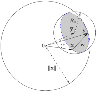
Figure 3: Schematic of the geometry of first-order perfect steganography.

Using the triangle inequality we can verify next that

$$\|\mathbf{w}\|=\|(\mathbf{y}-\overline{\mathbf{y}})-(\mathbf{x}-\overline{\mathbf{y}})\|\leq 2\|\mathbf{y}-\overline{\mathbf{y}}\|=2R_{s},$$ (20)

or, equivalently, that $\|\mathbf{w}\|$ cannot be greater than the diameter of the secondary permutation sphere. Using (18), we see that (20) implies the inequality

$$\|\mathbf{w}\|^{2}_{\mathrm{max}}\leq 2\overline{\|\mathbf{w}\|^{2}},$$ (21)

which supplements (12). A case in which equality holds in (21) is $\mathbf{x}=v\,\mathbf{1}$, but there may also exist other equality solutions with a nonconstant host. Inequality (21) also narrows down the probability bound in (16), since it implies that this probability can only be nonzero when $\gamma\in(0,1]$. Finally, when (21) is normalized by the power of the host we obtain

$$\xi_{\mathrm{min}}\geq\underline{\xi}/2,$$ (22)

which means that the host to maximum watermark power ratio is, in decibels, always greater or equal than the host to average watermark power ratio minus approximately $3$ dB.

An alternative proof of inequality (11) is found, for instance, by combining (20) and (19). This can also be seen directly by applying the triangle inequality as in (20) but with $\mathbf{0}$ instead of $\overline{\mathbf{y}}$, which is equivalent to saying that $\|\mathbf{w}\|$ cannot be greater than the diameter of the primary permutation sphere. Thus (11) is met with equality whenever there exist two antipodal codewords, that is to say, when there exist $\mathbf{y}$ and $\mathbf{y}^{\prime}$ such that $\mathbf{y}^{\prime}=-\mathbf{y}$. This happens when $\mathbf{x}^{\uparrow}=-\mathbf{x}^{\downarrow}$, two antipodal codewords being $\mathbf{y}={\mathbf{x}^{\uparrow}}$ and $\mathbf{y}^{\prime}={\mathbf{x}^{\downarrow}}$. In the special case in which $\mathbf{x}$ lies in the nonnegative (or nonpositive) orthant, the greatest possible diameter of the secondary permutation sphere allows us to replace (11) by $\|\mathbf{w}\|^{2}_{\mathrm{max}}\leq 2\|\mathbf{x}\|^{2}$ (and hence $\xi_{\mathrm{min}}\geq 1/2$), with equality when at least half of the elements of $\mathbf{x}$ are zero.

To conclude this section, it can also be observed that the host to average watermark power ratio can be expressed as a single function of the angle $\phi$ between $\mathbf{x}$ and $\mathbf{1}$ (equivalently, between any codeword $\mathbf{y}$ and $\mathbf{1}$). Since $\cos\phi=\mathbf{x}^{t}\mathbf{1}/\left(\|\mathbf{x}\|\|\mathbf{1}\|\right)$, it can be seen from (5) and (13) that

$$\underline{\xi}=\frac{1}{2\sin^{2}\phi}.$$ (23)

This expression also allows us to establish (22) without explicitly resorting to the secondary permutation sphere. Since the angle $2\phi$ is the opening angle of the right cone with apex $\mathbf{0}$ and base the intersection of the primary permutation sphere and the permutation plane, then the maximum distance between any codeword $\mathbf{y}$ and $\mathbf{x}$ is bounded as follows:

$$\|\mathbf{y}-\mathbf{x}\|^{2}\leq 2\|\mathbf{x}\|^{2}(1-\cos 2\phi).$$ (24)

Using next the trigonometric identity $\cos 2\phi=1-2\sin^{2}\phi$ and (23) in (24) we recover (22).

Some of the facts discussed in this section are schematically illustrated in Figure 3.

V-B Degree of host change

The degree of host change is an embedding distortion measure alternative to the squared Euclidean distance, which, as we will see, is also insightful in a number of ways. In this case the similarity measure is $s(\mathbf{x},\mathbf{y})=(1/n)\,\delta(\mathbf{y},\mathbf{x})=(1/n)\omega(\mathbf{w})$, that is to say, the Hamming distance per symbol between $\mathbf{y}$ and $\mathbf{x}$, or the fraction of elements of $\mathbf{y}$ which differ from the same index elements in $\mathbf{x}$. For simplicity, in the remainder we will use the notation $\nu\triangleq(1/n)\,\delta(\mathbf{y},\mathbf{x})$.

We will determine next the average degree of host change over all rearrangements ($\overline{\nu}$), in order to have a measurement independent of any particular $\mathbf{y}$. We firstly define an auxiliary $q\times n$ matrix $\Lambda$ whose entries are $(\Lambda)_{k,i}=\mathbbold{1}_{\{v_{k}=x_{i}\}}$, and we let $\Omega\triangleq\Lambda^{t}\Lambda$. Now, $\mathop{\rm tr}\Lambda\Pi_{\boldsymbol{\sigma}}\Lambda^{t}=\mathop{\rm tr}\Omega\Pi_{\boldsymbol{\sigma}}$ is the number of elements in $\mathbf{y}=\Pi_{\boldsymbol{\sigma}}\mathbf{x}$ unchanged with respect to $\mathbf{x}$. Therefore $\delta(\mathbf{y},\mathbf{x})=n-\mathop{\rm tr}\Omega\Pi_{\boldsymbol{\sigma}}$, and, when the messages are uniform, the average degree of host change can be put as

$$\overline{\nu}=\frac{1}{r}\sum_{\boldsymbol{\sigma}\in\mathcal{S}_{\mathbf{x}}}\frac{1}{n}(n-\mathop{\rm tr}\Omega\Pi_{\boldsymbol{\sigma}}).$$ (25)

We can develop this expression using the equality $(1/r)\sum_{\boldsymbol{\sigma}\in\mathcal{S}_{\mathbf{x}}}\mathop{\rm tr}\Omega\Pi_{\boldsymbol{\sigma}}=(1/n!)\sum_{\boldsymbol{\sigma}\in\mathcal{S}_{n}}\mathop{\rm tr}\Omega\Pi_{\boldsymbol{\sigma}}$, which holds because the second summation contains the same summands as the first one, but each of them repeated $h_{1}!h_{2}!\cdots h_{q}!$ times. As the trace operator is linear, using equation (69) and $\mathop{\rm tr}\Omega\mathbf{1}\mathbf{1}^{t}=\mathbf{1}^{t}\Omega\mathbf{1}=\|\Lambda\mathbf{1}\|^{2}=\|\mathbf{h}\|^{2}$, it can be seen that

$$\overline{\nu}=1-\frac{\|\mathbf{h}\|^{2}}{n^{2}}=1-\|\mathbf{p}\|^{2}.$$ (26)

As $\mathbf{p}$ (the type of $\mathbf{x}$) contains the probabilities of a pmf (whose support is $\mathbf{v}$) then $1/q\leq\|\mathbf{p}\|^{2}\leq 1$, and so we have that

$$0\leq\overline{\nu}\leq 1-\frac{1}{q}.$$ (27)

A useful probabilistic interpretation of (26) can be obtained as follows. Consider two independent discrete random variables whose distribution is the type of $\mathbf{x}$, which we denote as $X\sim\mathbf{p}$ and $Y\sim\mathbf{p}$. The complement of their index of coincidence, or, equivalently, the probability of drawing a different outcome in two independent trials of $X$ and $Y$, is $\Pr\{X\neq Y\}=\sum_{v\in\mathcal{V}}p(X=v)p(Y\neq v)$. This amount is

$$\Pr\{X\neq Y\} = \sum_{k=1}^{q}p_{k}\left(1-p_{k}\right)=\overline{\nu}.$$ (28)

As for the relationship between $\overline{\nu}$ and $\overline{\|\mathbf{w}\|^{2}}$, since $\delta(\mathbf{y},\mathbf{x})\leq\|\mathbf{y}-\mathbf{x}\|^{2}$ for $\mathbf{x},\mathbf{y}\in\mathbb{Z}^{n}$ then

$$\overline{\nu}\leq\frac{1}{n}\overline{\|\mathbf{w}\|^{2}},$$ (29)

The right-hand side of (29) can be greater than one, but the bound is tight when $\underline{\xi}\to\infty$; intuitively, a high $\underline{\xi}$ implies a small $\overline{\nu}$. Finally note that, unlike the $\xi$ ratios, $\overline{\nu}$ is not preserved, in general, by unitary linear transforms when $q>2$.

V-C Rate-distortion bounds

Ideally we would like to have exact rate-distortion relationships, that is to say, explicit or implicit equations relating the embedding rate $\rho$ discussed in Section IV-A and either $(1/n)\overline{\|\mathbf{w}\|^{2}}$ or $\overline{\nu}$. Leaving aside the asymptotic case of the binary Hamming setting which we discuss later in Section V-E, we suspect that, in general, such relationships do not exist. If they would, they could not simply involve the three aforementioned amounts. Two particular nonbinary hosts validating this observation are $\mathbf{x}=[1,2,3,4,4,4,4]^{t}$ and $\mathbf{x}^{\prime}=[1,1,2,2,3,3,3]^{t}$, which have the same $\rho$ but different $(1/n)\overline{\|\mathbf{w}\|^{2}}$ and $\overline{\nu}$.

Nevertheless, a general upper bound on $\rho$ solely based on $(1/n)\overline{\|\mathbf{w}\|^{2}}$ is possible using the differential entropy upper bound on discrete entropy, independently found by Djackov [24], Massey [25], and Willems (unpublished, see [18, Problem 8.7]). This bound is $H(X)<(1/2)\log(2\pi e(\sigma_{X}^{2}+1/12))$ for a discrete random variable $X$ with support set $\mathcal{V}\subseteq\mathbb{Z}$ and variance $\sigma_{X}^{2}$. Using the upper bound in (3), since $X\sim\mathbf{p}$ has support set $\mathcal{V}\subset\mathbb{Z}$ and variance $\sigma^{2}_{\mathbf{x}}$ [given in (7)], we have that the Djackov-Massey-Willems bound yields

$$\rho<\rho_{u}\triangleq\frac{1}{2}\log\left(2\pi e\left(\frac{\overline{\|\mathbf{w}\|^{2}}}{2n}+\frac{1}{12}\right)\right).$$ (30)

The bound is loose as $\overline{\|\mathbf{w}\|^{2}}/n\to 0$, as in this case $\rho_{u}\to 0.2546$ whereas we know that $\rho\to 0$. In practical terms, this effect only starts to be discernible when $\underline{\xi}^{\prime}\gtrapprox 50$ dB for $b=8$.

Also, from (28) and the upper bound in (3), another rate-distortion upper bound is directly given by Fano’s inequality:

$$\rho\leq\rho_{u}^{\prime}\triangleq h(\overline{\nu})+\log(q-1)\,\overline{\nu}.$$ (31)

Although it is well-known that the sharpest bound is achieved by any permutation of $\mathbf{p}=[1-\overline{\nu},\overline{\nu}/(q-1),\cdots,\overline{\nu}/(q-1)]^{t}$, note from (3) that this does not imply that $\rho=\rho_{u}^{\prime}$. Moreover the type $\mathbf{p}$ is fixed for the problem, and so this bound is generally loose.

Furthermore, it is possible to give two lower bounds on $\rho$ based on $\overline{\nu}$. The first one is based on inequality $\Pr\{X=Y\}\geq 2^{-H(X)}$ with $X$ and $Y$ i.i.d. [18, Lemma 2.10.1] Using the complement of the index of coincidence (28) and the lower bound in (3) in this inequality, we obtain

$$\rho\geq\rho_{l}\triangleq-\log(1-\overline{\nu})-\zeta^{(q,n)}.$$ (32)

Asymptotically, we have that $\rho_{l}\doteq-\log(1-\overline{\nu})$. Since the original bound is sharp when $X$ is uniform, asymptotic equality is achieved in inequality (32) when $\mathbf{h}=(n/q)\mathbf{1}$, and in this case $\rho=\rho_{l}\doteq\log q$, which corresponds to the maximum average degree of host change $\overline{\nu}=1-1/q$.

The second lower bound is obtained from inequality $H(X)\geq 2\Pr\{X\neq Y\}$ with $X$ and $Y$ i.i.d., found by Harremoës and Topsøe [26, Theorem II.6 with $k=1$]. Using again the lower bound in (3) and (28) we obtain

$$\rho\geq\rho_{l}^{\prime}\triangleq 2\,\overline{\nu}-\zeta^{(q,n)},$$ (33)

which is sharper than (32) when $0<\overline{\nu}<1/2$. The asymptotic bound is now $\rho_{l}^{\prime}\doteq 2\overline{\nu}$.

Finally, from (30), (32) and (33) we have two upper bounds on $\overline{\nu}$ based on $(1/n)\overline{\|\mathbf{w}\|^{2}}$ in addition to (29). If we define $\tau\triangleq 2^{\zeta^{(q,n)}}(2\pi e(\overline{\|\mathbf{w}\|^{2}}/2n+1/12))^{1/2}$, then from $\rho_{l}<\rho_{u}$ and from $\rho_{l}^{\prime}<\rho_{u}$ we respectively have that

$$\overline{\nu}<1-\frac{1}{\tau},\quad\text{and}\quad\overline{\nu}<\frac{1}{2}\log\tau.$$ (34)

The first upper bound in (34) cannot be greater than the unity, unlike the second upper bound or (29). However, as $\underline{\xi}\to\infty$ (29) is eventually tighter than both inequalities in (34), which is due to the lack of asymptotic sharpness of (30).

Since $\rho$, $\overline{\|\mathbf{w}\|^{2}}$ and $\overline{\nu}$ are completely determined by $\mathbf{x}$, the rate-distortion bounds presented in this section may look like little more than a curiosity at this juncture. However their relevance will become apparent when we address embedding distortion control for permutation coding in Section VI.

V-D Embedding efficiency

In this section we will study the average embedding efficiency ($\overline{\varepsilon}$) [27]. This quantity is defined as the average number of message bits embedded per host element change, and, hence, it simultaneously involves embedding rate and embedding distortion. The original idea behind $\overline{\varepsilon}$ was measuring the security of a steganographic algorithm: given two algorithms with the same $\rho$, the one with higher $\overline{\varepsilon}$ should be less detectable since, on average, it embeds the same amount of information with less degree of host change.

Since permutation coding leads to perfect steganography with finite memoryless hosts, it may seem that there is little point in contemplating $\overline{\varepsilon}$ here. However, we will see that the average embedding efficiency allows for an insightful comparison between permutation coding and model-based steganography [4]. Moreover, $\overline{\varepsilon}$ may also find application in realistic scenarios in which the memoryless assumption is only an approximation. The computation of $\overline{\varepsilon}$ will again require the $\Omega$ matrix defined in Section V-B. Firstly see that the embedding efficiency for the message encoded by $\mathbf{y}=\Pi_{\boldsymbol{\sigma}}\mathbf{x}$ is $\varepsilon\triangleq\log r/(n\nu)=\log r/(n-\mathop{\rm tr}\Omega\Pi_{\boldsymbol{\sigma}})$ bits/host element change. This amount is infinite for $\boldsymbol{\sigma}_{0}\in\mathcal{S}_{\mathbf{x}}$ such that $\Pi_{\boldsymbol{\sigma}_{0}}\mathbf{x}=\mathbf{x}$, which without loss of generality may be assumed to be $\boldsymbol{\sigma}_{0}\triangleq[1,2,\ldots,n]^{t}$. In order to sidestep this singularity we will consider that $\varepsilon=0$ when $\mathbf{y}=\mathbf{x}$. Therefore, when all messages are equally likely the average sought is

$$\overline{\varepsilon}=\frac{1}{r}\sum_{\boldsymbol{\sigma}\in\mathcal{S}_{\mathbf{x}}\backslash\boldsymbol{\sigma}_{0}}\frac{\log r}{n-\mathop{\rm tr}\Omega\Pi_{\boldsymbol{\sigma}}}\quad\text{bits/host element change}.$$ (35)

An exact evaluation of (35) requires enumerating the number of permutations associated to each possible value of $\mathop{\rm tr}\Omega\Pi_{\boldsymbol{\sigma}}$ for $\boldsymbol{\sigma}\in\mathcal{S}_{\mathbf{x}}\backslash\boldsymbol{\sigma}_{0}$, namely $\{0,1,2,\ldots,n-2\}$ ($n-1$ is not a possible value because an elementary permutation involves swapping two indices). Obtaining this enumeration is equivalent to solving a generalization of the classic problem of rencontres [28], which asks for the number of $\boldsymbol{\sigma}\in\mathcal{S}_{n}$ that exhibit a given number of fixed points with respect to ${\boldsymbol{\sigma}}_{0}$. The generalized problem at hand requires instead finding the number of rearrangements of $\mathbf{x}$ that exhibit a given number of fixed points with respect to $\mathbf{x}$. We are not aware of a solution to this generalized problem, but a useful lower bound on $\overline{\varepsilon}$ can be found by observing that (35) involves the harmonic mean of $r-1$ positive values, which is bounded from above by their arithmetic mean [23]. Then we have that

$$\overline{\varepsilon}\geq\overline{\varepsilon}_{l}\triangleq n\rho\left(\frac{r-1}{r}\right)\left(\frac{1}{r-1}\sum_{\boldsymbol{\sigma}\in\mathcal{S}_{\mathbf{x}}\backslash\boldsymbol{\sigma}_{0}}\left(n-\mathop{\rm tr}\Omega\Pi_{\boldsymbol{\sigma}}\right)\right)^{-1}.$$ (36)

As the sum over $\boldsymbol{\sigma}\in\mathcal{S}_{\mathbf{x}}\backslash\boldsymbol{\sigma}_{0}$ in (36) is equal to the same sum over $\boldsymbol{\sigma}\in\mathcal{S}_{\mathbf{x}}$ we can see using (25) that

$$\overline{\varepsilon}_{l}=\left(\frac{r-1}{r}\right)^{2}\,\frac{\rho}{\overline{\nu}}.$$ (37)

Recalling the lower bound in (3) we can in turn bound (37) from below as follows: $\overline{\varepsilon}_{l}\geq\overline{\varepsilon}_{l}^{\prime}\triangleq((r-1)/r)^{2}(H(X)-\zeta^{(q,n)})/\overline{\nu}$. In the following we will consider the asymptotics of $\overline{\varepsilon}_{l}^{\prime}$ as $n\to\infty$. As in this case $(r-1)/r\to 1$ we have that

$$\overline{\varepsilon}_{l}^{\prime}\doteq\frac{-\sum_{k=1}^{q}p_{k}\log p_{k}}{1-\sum_{k=1}^{q}p_{k}^{2}}.$$ (38)

A basic but loose lower bound on (38) can be found by applying the well-known inequality $p-1\geq\log_{e}p$ to every logarithm in the numerator of the expression, which yields $\overline{\varepsilon}_{l}^{\prime}\;\shortstack[c]{\vspace*{-.05cm}.\\ $>$}\;1/(\log_{e}2)\approx 1.44$, but the sharpest lower bound is obtained by applying to (38) the same inequality from [26] used to obtain (33), which yields the asymptotic lower bound

$$\overline{\varepsilon}_{l}^{\prime}\;\shortstack[c]{\vspace*{-.05cm}.\\ $\geq$}\;2.$$ (39)

Consequently, a minimum average embedding efficiency of $2$ bits/host element change is asymptotically guaranteed when using permutation coding.

V-E Binary host

We now particularize and expand some of the previous results for the special case $q=2$. This case may arise because the host is intrinsically binary or, as we will discuss in Section VI, because we are dealing with a two-valued partition of a nonbinary host (see Section VI-B2). In the binary case the number of rearrangements (1) is given by the binomial coefficient $r={n\choose h_{2}}=n!/\left((n-h_{2})!h_{2}!\right)$, and (38) becomes

$$\overline{\varepsilon}_{l}^{\prime}\doteq\frac{-(1-p_{2})\log(1-p_{2})-p_{2}\log p_{2}}{2\,p_{2}(1-p_{2})}.$$

This same expression was previously given by Sallee [4, page 11] for the average embedding efficiency of model-based steganography with quantizer step size 2 (by which Sallee means a two-valued partitioning of a host signal using adjacent pairs of histogram bins), although we have proved here that it is only an asymptotic lower bound. Inequality (39) was also mentioned in [4], but the justification therein is, apparently, only empirical and restricted to the binary case —note that our conclusion is based on the aforementioned theoretical result by Harremoës and Topsøe [26], which holds for arbitrary $q$. We will return to the connection between permutation coding and model-based steganography, already hinted by (2), in Section VI-B2.

Hamming distance

An even more particular binary case is the one which the support set of the host is $\mathcal{V}=\{0,1\}$. In this case it is quite natural to measure the embedding distortion using the Hamming distance. Incidentally, the squared Euclidean distance between two vectors $\mathbf{x},\mathbf{y}\in\{0,1\}^{n}$ is equal to their Hamming distance or to the Hamming weight of the watermark, that is to say, $\delta(\mathbf{y},\mathbf{x})=\|\mathbf{y}-\mathbf{x}\|^{2}=\|\mathbf{w}\|^{2}=\omega(\mathbf{w})$. Therefore, the average degree of host change is completely equivalent to distortion measures based on the squared Euclidean distance: letting $\overline{\omega(\mathbf{w})}=\overline{\|\mathbf{w}\|^{2}}$, from the previous considerations it now holds that

$$\frac{1}{n}\,\overline{\omega(\mathbf{w})}=\overline{\nu}.$$ (40)

Also the Hamming weight of $\mathbf{x}$ is now equal to its squared norm, $\omega(\mathbf{x})=\|\mathbf{x}\|^{2}$. A further identity that holds true in this case is $\|\mathbf{x}\|^{2}=\mathbf{x}^{t}\mathbf{1}$. As a consequence of these facts, the theoretical analyses in Sections V-A and V-B can be particularized, and new rate-distortion results can be found. Firstly see that (5) (or equivalently $n\,\overline{\nu}$) becomes

$$\overline{\omega(\mathbf{w})}=2\omega(\mathbf{x})\left(1-\frac{1}{n}\omega(\mathbf{x})\right).$$ (41)

Considering (40) and (27), it now holds that $(1/n)\overline{\omega(\mathbf{w})}\leq 1/2$ with equality when $(1/n)\omega(\mathbf{x})=1/2$. On the other hand, (10) now takes the form

$$\omega(\mathbf{w})_{\mathrm{max}}=2\min(\omega(\mathbf{x}),n-\omega(\mathbf{x})).$$ (42)

Using (41) and (42), the figures of merit for the embedding distortion (13) and (14) can be put as a function of $\overline{\omega}(\mathbf{x})\triangleq(1/n)\omega(\mathbf{x})=p_{2}$ as follows:

$$\underline{\xi}=\frac{1}{2(1-\overline{\omega}(\mathbf{x}))},$$ (43)

$$\xi_{\mathrm{min}}=\frac{1}{2}\max\left(1,\frac{\overline{\omega}(\mathbf{x})}{1-\overline{\omega}(\mathbf{x})}\right)$$ (44)

whereas $\underline{\xi}^{\prime}=1/\left(2\overline{\omega}(\mathbf{x})(1-\overline{\omega}(\mathbf{x}))\right)=1/\overline{\nu}$. The inequalities in (14) must still hold; additionally, we have from (27) that $\underline{\xi}\geq 2\,\overline{\omega}(\mathbf{x})$. Since $\mathbf{x}$ is in the nonnegative orthant, we can see that $\xi_{\mathrm{min}}\geq 1/2$, with equality when $\overline{\omega}(\mathbf{x})\leq 1/2$ (as discussed in Section V-A3). Although (22) must still hold, we can now combine (43) and (44) to obtain the following exact relationship between these two amounts:

$$\xi_{\mathrm{min}}=\frac{1}{2}\max\left(1,2\underline{\xi}-1\right).$$

Finally, in the binary Hamming case we have from (3) that $\rho\leq h(p_{2})$. Therefore we have an exact relationship between the asymptotic embedding rate $\rho\doteq h(p_{2})=h(\overline{\omega}(\mathbf{x}))$ and the average embedding distortion (40) since both these amounts only depend on $\overline{\omega}(\mathbf{x})$. Thus the rate-distortion bounds in Section V-C, although still valid, are asymptotically unnecessary in this case. In any case (30) is not useful now, as it can be greater than one; on the other hand Fano’s inequality (31) now becomes

$$\rho\leq h(\overline{\nu}).$$ (45)

This bound, deduced here for permutation coding with binary base vector $\mathbf{x}$, was previously reported to hold for general binary block codes in [29, Theorem 1]. Also (45) can be tightened in this case using the well-known inequality of the binary entropy function $h(p_{2})\leq 2\sqrt{p_{2}(1-p_{2})}$, which allows us to write the non-asymptotic rate-distortion upper bound

$$\rho\leq\rho_{u}^{\prime\prime}\triangleq\sqrt{2\overline{\nu}},$$ (46)

which is sharper than (45) when $\overline{\nu}\in(0.077,1/2)$.

VI Embedding Distortion Control

As argued in Section III, practical universal steganography requires enforcing similarity between $\mathbf{x}$ and $\mathbf{y}$ (see Figure 1). Nonetheless, a permutation code based on $\mathbf{x}$ —a fixed input parameter for the encoder— does not ensure by itself compliance with some pre-established embedding distortion constraint, such as for instance a constraint on the maximum value of $\overline{\nu}$ or on the minimum value of $\underline{\xi}$. Critically, we discussed in Section V-A1 that $\underline{\xi}$ can be very low. However similarity between $\mathbf{x}$ and $\mathbf{y}$ can be increased by restricting the encoding to a judiciously chosen subset of the set of all permutation codewords. In this section we introduce and analyze partitioned permutation coding, which enables embedding distortion control by means of a similarity increasing strategy based on the principle just mentioned.

Definitions

A partitioning (or regular partitioning) is defined to be a set of $p$ index vectors $\mathcal{U}_{n}^{p}=\{\mathbf{u}_{1},\mathbf{u}_{2},\ldots,\mathbf{u}_{p}\}$ such that: 1) $[\mathbf{u}_{1}^{t},\mathbf{u}_{2}^{t},\ldots,\mathbf{u}_{p}^{t}]^{t}\in\mathcal{S}_{n}$; and 2) $\mathbf{u}_{j}={\mathbf{u}^{\uparrow}_{j}}$. Consequently, the lengths $n_{1},n_{2},\ldots,n_{p}$ of $\mathbf{u}_{1},\mathbf{u}_{2},\ldots,\mathbf{u}_{p}$ fulfill $\sum_{j=1}^{p}n_{j}=n$. A partitioning $\mathcal{U}_{n}^{p}$ is applied to an $n$-vector $\mathbf{x}$ by forming $p$ partitions $\mathbf{x}_{1},\mathbf{x}_{2},\ldots,\mathbf{x}_{p}$, which are vectors formed by elements of $\mathbf{x}$ indexed by the index vectors. Thus, for $j=1,2,\ldots,p$ the elements of partition $\mathbf{x}_{j}$ are $(\mathbf{x}_{j})_{i}=(\mathbf{x})_{(\mathbf{u}_{j})_{i}}$ with $i=1,2,\ldots,n_{j}$. The application of partitioning $\mathcal{U}_{n}^{p}$ to $\mathbf{x}$ is denoted by $\mathcal{U}_{n}^{p}(\mathbf{x})=\{\mathbf{x}_{1},\mathbf{x}_{2},\ldots,\mathbf{x}_{p}\}$, which will also be referred to as a partitioning of $\mathbf{x}$.

A support partitioning is defined to be a partitioning $\mathcal{U}_{q}^{p}$, which is to be applied to the support $q$-vector $\mathbf{v}$. A partitioning of $\mathbf{v}$, i.e., $\mathcal{U}_{q}^{p}(\mathbf{v})=\{\mathbf{v}_{1},\mathbf{v}_{2},\ldots,\mathbf{v}_{p}\}$, can be used in turn to build a support-induced partitioning of $\mathbf{x}$, which we denote by $\mathcal{U}_{n}^{p}(\mathcal{U}_{q}^{p},\mathbf{x})=\{\mathbf{x}_{1},\mathbf{x}_{2},\ldots,\mathbf{x}_{p}\}$. This is obtained through the application to $\mathbf{x}$ of a regular partitioning $(\mathcal{U}^{p}_{n})^{\star}$ dependent on $\mathcal{U}_{q}^{p}(\mathbf{v})$ and on $\mathbf{x}$, whose index vector $\mathbf{u}^{\star}_{j}$ contains all indices $i$ such that $x_{i}=(\mathbf{v}_{j})_{k}$, where $1\leq i\leq n$ and $1\leq k\leq n_{j}$. Hence $\mathcal{U}_{n}^{p}(\mathcal{U}_{q}^{p},\mathbf{x})=(\mathcal{U}^{p}_{n})^{\star}(\mathbf{x})$.

The partitions in $\mathcal{U}_{q}^{p}(\mathbf{v})$ necessarily coincide with the supports of the partitions in $\mathcal{U}_{n}^{p}(\mathcal{U}_{q}^{p},\mathbf{x})$. Therefore the lengths $q_{1},q_{2},\ldots,q_{p}$ of $\mathbf{v}_{1},\mathbf{v}_{2},\ldots,\mathbf{v}_{p}$ fulfill $\sum_{j=1}^{p}q_{j}=q$, not only for $\mathcal{U}_{q}^{p}(\mathbf{v})$ (by the definition of partitioning) but also for the lengths of the supports of the partitions in $\mathcal{U}_{n}^{p}(\mathcal{U}_{q}^{p},\mathbf{x})$. Note that for a regular partitioning of $\mathbf{x}$ [i.e., $\mathcal{U}_{n}^{p}(\mathbf{x})$] we have instead that $\sum_{j=1}^{p}q_{j}\geq q$, because it is possible that the same support value $v\in\mathcal{V}$ may be found in more than one partition of $\mathbf{x}$.

Example 1: In order to clarify these concepts, consider the host $\mathbf{x}=[v_{1},v_{3},v_{2},v_{3},v_{1},v_{3}]^{t}$ with support $\mathbf{v}=[v_{1},v_{2},v_{3}]^{t}$ and histogram $\mathbf{h}=[2,1,3]^{t}$ ($q=3$). An example of a possible regular partitioning is $\mathcal{U}_{6}^{2}=\{\mathbf{u}_{1},\mathbf{u}_{2}\}$ with index vectors $\mathbf{u}_{1}=[2,3,4,5]^{t}$ and $\mathbf{u}_{2}=[1,6]^{t}$ which yields $\mathcal{U}_{6}^{2}(\mathbf{x})=\{\mathbf{x}_{1},\mathbf{x}_{2}\}$ with partitions $\mathbf{x}_{1}=[v_{3},v_{2},v_{3},v_{1}]^{t}$ and $\mathbf{x}_{2}=[v_{1},v_{3}]^{t}$. The supports of these partitions are $\mathbf{v}_{1}=[v_{1},v_{2},v_{3}]^{t}$ ($q_{1}=3$) and $\mathbf{v}_{2}=[v_{1},v_{3}]^{t}$ ($q_{2}=2$), and thus $q_{1}+q_{2}>q$.

An example of a possible support partitioning is $\mathcal{U}_{3}^{2}=\{\mathbf{u}_{1}^{\prime},\mathbf{u}_{2}^{\prime}\}$ with index vectors $\mathbf{u}_{1}^{\prime}=[1,2]^{t}$ and $\mathbf{u}_{2}^{\prime}=[3]$ which yields $\mathcal{U}_{3}^{2}(\mathbf{v})=\{\mathbf{v}_{1}^{\prime},\mathbf{v}_{2}^{\prime}\}$ with partitions $\mathbf{v}_{1}^{\prime}=[v_{1},v_{2}]^{t}$ and $\mathbf{v}_{2}^{\prime}=[v_{3}]$. In this case $(\mathcal{U}_{6}^{2})^{\star}$ contains ${\mathbf{u}_{1}^{\star}}^{\prime}=[1,3,5]^{t}$ and ${\mathbf{u}_{2}^{\star}}^{\prime}=[2,4,6]^{t}$, and so $\mathcal{U}_{6}^{2}(\mathcal{U}_{3}^{2},\mathbf{x})=(\mathcal{U}_{6}^{2})^{\star}(\mathbf{x})=\{\mathbf{x}_{1}^{\prime},\mathbf{x}_{2}^{\prime}\}$ contains partitions $\mathbf{x}_{1}^{\prime}=[v_{1},v_{2},v_{1}]^{t}$ and $\mathbf{x}_{2}^{\prime}=[v_{3},v_{3},v_{3}]^{t}$. The lengths of the support partitions $\mathbf{v}_{1}^{\prime}$ and $\mathbf{v}_{2}^{\prime}$ (which are also the supports of $\mathbf{x}_{1}^{\prime}$ and $\mathbf{x}_{2}^{\prime}$) are $q_{1}^{\prime}=2$ and $q_{2}^{\prime}=1$, and thus $q_{1}^{\prime}+q_{2}^{\prime}=q$.

Partitioned permutation coding

The previous definitions suffice to describe partitioned permutation coding. Encoder and decoder share a partitioning $\mathcal{U}_{n}^{p}$. The encoder obtains $\mathcal{U}_{n}^{p}(\mathbf{x})$ and then undertakes permutation coding separately on each of the $p$ partitions; in short, it produces $\mathbf{y}_{j}=\Pi_{\boldsymbol{\sigma}_{j}}\mathbf{x}_{j}$ with $\boldsymbol{\sigma}_{j}\in\mathcal{S}_{\mathbf{x}_{j}}$ for $j=1,2,\ldots,p$. In practice, $\mathbf{y}_{j}$ is produced by undertaking adaptive arithmetic decoding of $\lfloor\log r_{j}\rfloor$ bits of the message to be embedded, relying on the histogram $\mathbf{h}_{j}$ of $\mathbf{x}_{j}$ as described in Section IV-B. The elements of vector $\mathbf{y}$ are obtained by piecing together all $\mathbf{y}_{j}$ partitions, and so $(\mathbf{y})_{(\mathbf{u}_{j})_{i}}=(\mathbf{y}_{j})_{i}$ with $i=1,2,\ldots,n_{j}$, for $j=1,2,\ldots,p$. The vector $\mathbf{y}$ thus obtained still preserves the histogram of $\mathbf{x}$ because it stems from permutations of partitions of $\mathbf{x}$, and hence $\mathbf{y}=\Pi_{\boldsymbol{\sigma}}\mathbf{x}$ for some $\boldsymbol{\sigma}\in\mathcal{S}_{\mathbf{x}}$. The decoder obtains $\mathcal{U}_{n}^{p}(\mathbf{y})$ and then, for $j=1,2,\ldots,p$, it undertakes adaptive arithmetic encoding of partition $\mathbf{y}_{j}$ relying on its histogram $\mathbf{h}_{j}$, thus retrieving all $p$ parts of the message.

Alternatively, encoder and decoder may share a support partitioning $\mathcal{U}_{q}^{p}$ instead of a regular partitioning $\mathcal{U}_{n}^{p}$. In this case the encoder generates $\mathbf{y}$ from $\mathcal{U}_{n}^{p}(\mathcal{U}_{q}^{p},\mathbf{x})$, and the decoder retrieves the message in $\mathbf{y}$ using $\mathcal{U}_{n}^{p}(\mathcal{U}_{q}^{p},\mathbf{y})$.

VI-A Theoretical analysis of partitioned permutation coding

Before proceeding, we need to rederive the most relevant results in Sections IV-A and V for partitioned permutation coding with a generic partitioning $\mathcal{U}^{p}_{n}$. Our computations will explicitly use $\mathcal{U}^{p}_{n}(\mathbf{x})=\{\mathbf{x}_{1},\mathbf{x}_{2},\ldots,\mathbf{x}_{p}\}$, which is the point of view of the encoder. However, be aware that we may also evaluate the theoretical expressions that we will obtain using instead $\mathcal{U}^{p}_{n}(\mathbf{y})=\{\mathbf{y}_{1},\mathbf{y}_{2},\ldots,\mathbf{y}_{p}\}$ for any rearrangement $\mathbf{y}$, which would be the point of view of the decoder.

Firstly, the number of embeddable messages is

$$r=\prod_{j=1}^{p}r_{j},$$ (47)

where $r_{j}={n_{j}\choose\mathbf{h}_{j}}$ is the multinomial coefficient associated to partition $\mathbf{x}_{j}$. Hence, the theoretical embedding rate $\rho=(1/n)\log r$ can be expressed as

$$\rho=\sum_{j=1}^{p}\frac{n_{j}}{n}\rho_{j},$$ (48)

where $\rho_{j}=(1/n_{j})\log r_{j}$ is the embedding rate for the $j$-th partition.

As for the embedding distortion results, firstly see that the average watermark power for partitioned permutation coding is $\overline{\|\mathbf{w}\|^{2}}=(1/r)\sum_{m_{1}=1}^{r_{1}}\cdots\sum_{m_{p}=1}^{r_{p}}\sum_{j=1}^{p}\|\mathbf{w}_{j}^{(m_{j})}\|^{2}$, where $\mathbf{w}_{j}^{(m_{j})}=\mathbf{y}_{j}^{(m_{j})}-\mathbf{x}_{j}$. This amount can be developed as follows

$$\overline{\|\mathbf{w}\|^{2}} = \sum_{j=1}^{p}\frac{1}{r}\Bigg{(}\prod_{i=1\above 0.0pti\neq j}^{p}r_{i}\Bigg{)}\sum_{m_{j}=1}^{r_{j}}\|\mathbf{w}_{j}^{(m_{j})}\|^{2}=\sum_{j=1}^{p}\overline{\|\mathbf{w}_{j}\|^{2}},$$

and hence

$$\overline{\|\mathbf{w}\|^{2}}=2\,\Bigg{(}\|\mathbf{x}\|^{2}-\sum_{j=1}^{p}\frac{1}{n_{j}}(\mathbf{x}^{t}_{j}\mathbf{1})^{2}\Bigg{)}.$$ (50)

In parallel to (7), the average watermark power per host element can be put in terms of the sample variances per partition, $\sigma^{2}_{\mathbf{x}_{j}}=\overline{\|\mathbf{w}_{j}\|^{2}}/(2n_{j})$, as follows:

$$\frac{1}{n}\overline{\|\mathbf{w}\|^{2}}=2\sum_{j=1}^{p}\frac{n_{j}}{n}\;\sigma^{2}_{\mathbf{x}_{j}}.$$ (51)

The maximum watermark power is obtained when $\|\mathbf{w}_{j}\|^{2}$ is maximum for all $j=1,2,\ldots,p$, and then $\|\mathbf{w}\|^{2}_{\mathrm{max}}=\sum_{j=1}^{p}(\|\mathbf{w}_{j}\|^{2})_{\mathrm{max}}$. Thus, we have that

$$\|\mathbf{w}\|^{2}_{\mathrm{max}}=2\,\left(\|\mathbf{x}\|^{2}-\sum_{j=1}^{p}{{\mathbf{x}^{\uparrow}_{j}}}^{t}{\mathbf{x}^{\downarrow}_{j}}\right).$$ (52)

From expressions (50) and (52) one obtains the figures of merit $\underline{\xi}$ ($\underline{\xi}^{\prime}$) and $\xi_{\mathrm{min}}$ for the partitioned problem (see definitions in Section V-A1). Importantly, inequalities (14) and (22) still hold with partitioned permutation coding, because inequalities (12) and (21) hold for the average and maximum of $\|\mathbf{w}_{j}\|^{2}$, for every $j=1,2,\ldots,p$.

The number of host changes caused within the $j$-th partition by permutation $\boldsymbol{\sigma}_{j}\in\mathcal{S}_{\mathbf{x}_{j}}$ is computed using a $q_{j}\times n_{j}$ matrix $\Lambda_{j}$ defined just like $\Lambda$ in Section V-B but using partitions $\mathbf{v}_{j}$ and $\mathbf{x}_{j}$. Hence, using $\Omega_{j}=\Lambda_{j}^{t}\Lambda_{j}$, for $j=1,2,\ldots,p$, we can write the average degree of host change for partitioned permutation coding as $\overline{\nu}=(1/r)\sum_{\boldsymbol{\sigma}_{1}\in\mathcal{S}_{\mathbf{x}_{1}}}\cdots\sum_{\boldsymbol{\sigma}_{p}\in\mathcal{S}_{\mathbf{x}_{p}}}(1/n)\left(\sum_{j=1}^{p}n_{j}-\mathop{\rm tr}\Omega_{j}\Pi_{\boldsymbol{\sigma}_{j}}\right)$. This expression can be developed like (VI-A) to yield

$$\overline{\nu} = \sum_{j=1}^{p}\frac{1}{r}\Bigg{(}\prod_{i=1\above 0.0pti\neq j}^{p}r_{i}\Bigg{)}\sum_{\boldsymbol{\sigma}_{j}\in\mathcal{S}_{\mathbf{x}_{j}}}\frac{1}{n}\left(n_{j}-\mathop{\rm tr}\Omega_{j}\Pi_{\boldsymbol{\sigma}_{j}}\right)=\sum_{j=1}^{p}\frac{n_{j}}{n}\;\overline{\nu}_{j},$$

where $\overline{\nu}_{j}=1-(\|\mathbf{h}_{j}\|/n_{j})^{2}=1-\|\mathbf{p}_{j}\|^{2}$.

Finally, the average embedding efficiency for partitioned permutation coding is

$$\overline{\varepsilon}=\frac{1}{r}\sum_{\boldsymbol{\sigma}_{1},\ldots,\boldsymbol{\sigma}_{p}\backslash\boldsymbol{\sigma}_{0}}\frac{\log r}{\sum_{j=1}^{p}n_{j}-\mathop{\rm tr}\Omega_{j}\Pi_{\boldsymbol{\sigma}_{j}}}.$$ (54)

The first summation in (54) ranges over all $\boldsymbol{\sigma}_{j}\in\mathcal{S}_{\mathbf{x}_{j}}$, for $j=1,2,\ldots,p$, bar the case $\boldsymbol{\sigma}_{0}\in\mathcal{S}_{\mathbf{x}}$ in which $\mathbf{y}=\mathbf{x}$. Using the same bounding strategy as in Section V-D, the lower bound $\overline{\varepsilon}_{l}$ to (54) is again (37), where $r$, $\rho$ and $\overline{\nu}$ are now given by (47), (48) and (VI-A), respectively. It can also be verified by applying (33) to each $\rho_{j}$ that (39) also holds for partitioned permutation coding.

We verify next that the rate-distortion bounds in Section V-C still hold. Applying (30) individually to the partition rates $\rho_{j}$ in (48), and then using the concavity of $\log(\cdot)$ and Jensen’s inequality, we have that

$$\rho < \sum_{j=1}^{p}\frac{n_{j}}{n}\;\frac{1}{2}\log\left(2\pi e\;\left(\sigma^{2}_{\mathbf{x}_{j}}+\frac{1}{12}\right)\right)$$ (55)

$$\leq \frac{1}{2}\log\left(2\pi e\;\sum_{j=1}^{p}\frac{n_{j}}{n}\left(\sigma^{2}_{\mathbf{x}_{j}}+\frac{1}{12}\right)\right).$$ (56)

Therefore, using (51) in (56) we recover (30). Note that the inequality leading to (56) (Jensen’s inequality) is met with equality if and only if $\sigma^{2}_{\mathbf{x}_{j}}=\overline{\|\mathbf{w}\|^{2}}/(2n)$ for all $j=1,2,\ldots,p$. Similarly, applying (31) individually to each $\rho_{j}$ in (48) and then using the concavity of $h(\overline{\nu}_{j})+\log(q_{j}-1)\,\overline{\nu}_{j}$ on $\overline{\nu}_{j}$, $\log q_{j}\leq\log q$, Jensen’s inequality and (VI-A), we see that (31) still holds with partitioning.

We finally prove that the rate-distortion lower bounds (32) and (33) also hold for the class of support-induced partitionings. Applying (32) individually to the partition rates $\rho_{j}$ in (48), and then using the convexity of $-\log(\cdot)$ and Jensen’s inequality, we have that

$$\rho \geq \sum_{j=1}^{p}\frac{n_{j}}{n}\;\left(-\log\left(1-\overline{\nu}_{j}\right)-\zeta^{(q_{j},n_{j})}\right)$$

$$\geq -\log\left(\sum_{j=1}^{p}\frac{n_{j}}{n}(1-\overline{\nu}_{j})\right)-\frac{q}{n}\log\left(\sum_{j=1}^{p}\frac{q_{j}}{q}n_{j}+1\right),$$

because $\sum_{j=1}^{p}(q_{j}/q)=1$ for support-induced partitionings. Therefore, using (VI-A) and $\sum_{j=1}^{p}(q_{j}/q)n_{j}\leq n$ in (LABEL:eq:bound-rate-dhc-part) we recover (32). Following the same steps as in (VI-A) and (LABEL:eq:bound-rate-dhc-part), it is seen that (33) still holds for support-induced partitionings.

Lastly, we describe the invariance property of support partitionings with respect to the theoretical analysis in this Section VI-A, which will be seen to be key for the optimization of partitioned permutation coding in Section VI-B. As discussed therein, this property allows the decoder to determine the partition dynamically chosen by the encoder in order to meet a distortion constraint, without the need for a side channel for the encoder to communicate its choice to the decoder.

Property (Invariance of support partitionings)

Given a support partitioning $\mathcal{U}_{q}^{p}$ and any arbitrary rearrangement $\mathbf{y}$ of the host $\mathbf{x}$, all theoretical predictions for partitioned permutation coding are identical when using either the support-induced partitioning $\mathcal{U}_{n}^{p}(\mathcal{U}_{q}^{p},\mathbf{x})$ or the support-induced partitioning $\mathcal{U}_{n}^{p}(\mathcal{U}_{q}^{p},\mathbf{y})$. In particular, there is always agreement between both cases on (48), (50), (52) and (VI-A), and consequently also on $\overline{\varepsilon}_{l}$ and all bounds (30–33) which we have seen always hold for support-induced partitionings. This behavior is due to the fact that, since the support partitions $\mathbf{v}_{1},\mathbf{v}_{2},\ldots,\mathbf{v}_{p}$ must be identical for any two partitionings induced by $\mathcal{U}_{q}^{p}$, then $\mathbf{y}_{j}$ must always be a rearrangement of $\mathbf{x}_{j}$ for $j=1,2,\ldots,p$. Seeing that all expressions (47–VI-A) are independent of any particular rearrangement of the values within any of the $p$ partitions, and that all rate-distortion bounds in Section V-C hold for support-induced partitionings, then it follows that the evaluation of every theoretical expression using $\mathcal{U}_{n}^{p}(\mathcal{U}_{q}^{p},\mathbf{x})$ or $\mathcal{U}_{n}^{p}(\mathcal{U}_{q}^{p},\mathbf{y})$ coincides.

We must remark that the invariance property does not hold in general for a regular partitioning $\mathcal{U}_{n}^{p}$. In this case, theoretical predictions using $\mathcal{U}_{n}^{p}(\mathbf{x})$ and $\mathcal{U}_{n}^{p}(\mathbf{y})$ only necessarily coincide in the particular case in which $\mathbf{y}$ stems from applying partitioned permutation coding to $\mathbf{x}$ using $\mathcal{U}_{n}^{p}$ (as in this case $\mathbf{y}_{j}$ must be a rearrangement of $\mathbf{x}_{j}$ for $j=1,2,\ldots,p$).

Example 2: Consider again the host $\mathbf{x}$ and the partitionings $\mathcal{U}_{6}^{2}$ and $\mathcal{U}_{3}^{2}$ given in Example 1. In order to numerically illustrate the invariance property of support partitionings, assume that $\mathbf{v}=[1,2,3]^{t}$, and consider the rearrangement $\mathbf{y}=[2,1,3,3,3,1]^{t}$ of $\mathbf{x}=[1,3,2,3,1,3]^{t}$. If the theoreticals are computed using $\mathcal{U}_{6}^{2}(\mathbf{x})=\{[3,2,3,1]^{t},[1,3]^{t}\}$, the main results are $\rho=4.58$, $\overline{\|\mathbf{w}\|^{2}}=9.5$, $\|\mathbf{w}\|^{2}_{\text{max}}=18$, $\overline{\varepsilon}_{l}=1$, and $\overline{\nu}=0.59$; however, the values obtained using $\mathcal{U}_{6}^{2}(\mathbf{y})=\{[1,3,3,3]^{t},[2,1]^{t}\}$ are different: $\rho=3$, $\overline{\|\mathbf{w}\|^{2}}=7$, $\|\mathbf{w}\|^{2}_{\text{max}}=10$, $\overline{\varepsilon}_{l}=0.92$, and $\overline{\nu}=0.42$. As $\mathbf{y}$ does not stem from $\mathcal{U}_{6}^{2}(\mathbf{x})$, no invariance is guaranteed. However, even though $\mathbf{y}$ does not stem from $\mathcal{U}_{6}^{2}(\mathcal{U}_{3}^{2},\mathbf{x})$ either, the results are identical for the support-induced partitionings $\mathcal{U}_{6}^{2}(\mathcal{U}_{3}^{2},\mathbf{x})=\{[1,2,1]^{t},[3,3,3]^{t}\}$ and $\mathcal{U}_{6}^{2}(\mathcal{U}_{3}^{2},\mathbf{y})=\{[2,1,1]^{t},[3,3,3]^{t}\}$: $\rho=1.58$, $\overline{\|\mathbf{w}\|^{2}}=1.33$, $\|\mathbf{w}\|^{2}_{\text{max}}=2$, $\overline{\varepsilon}_{l}=0.19$, and $\overline{\nu}=0.23$ (i.e., we observe the invariance property of support partitionings). Notice that in $\mathcal{U}_{6}^{2}(\mathbf{x})$ and $\mathcal{U}_{6}^{2}(\mathbf{y})$ the partitions are not rearrangements of each other, whereas in $\mathcal{U}_{6}^{2}(\mathcal{U}_{3}^{2},\mathbf{x})$ and $\mathcal{U}_{6}^{2}(\mathcal{U}_{3}^{2},\mathbf{y})$ they are (in this toy example, the second partition is identical in both cases).

VI-B Static and adaptive partitioning

As we have seen, encoder and decoder can always implement partitioned permutation coding by sharing a partitioning $\mathcal{U}_{n}^{p}$ (or else a support partitioning $\mathcal{U}_{q}^{p}$). This strategy will lead to an embedding distortion which may or may not comply with a given constraint. Since in this case the shared partitioning is predetermined, we will call this strategy static partitioning.

For partitioned permutation coding to comply with a distortion constraint, adaptive partitioning is required. Adaptive partitioning is an optimization problem where a partitioning $\mathcal{U}_{n}^{p}$ must be chosen for host $\mathbf{x}$ such that the constraint is met and the embedding rate is maximized. In the following we will only consider a maximum constraint on $\overline{\|\mathbf{w}\|^{2}}$ (equivalently, a minimum constraint on $\underline{\xi}$ or on $\underline{\xi}^{\prime}$). The reason is twofold: 1) the average watermark power asymptotically approximates the watermark power associated to any random rearrangement of $\mathbf{x}$ (Section V-A2), and it also bounds the maximum power through (22); and 2) from (29) and (34) one sees that a maximum constraint on $\overline{\|\mathbf{w}\|^{2}}$ implies a maximum constraint on $\overline{\nu}$, whereas $\overline{\|\mathbf{w}\|^{2}}$ is more convenient to assess the suitability of a partitioning via the rate-distortion upper bound (30). With these considerations in mind, adaptive partitioning involves solving the optimization problem

$$\rho^{*}=\max_{\mathcal{U}_{n}^{p}(\mathbf{x}):\;\underline{\xi}\,\geq\kappa}\rho,$$ (59)

where $\rho$ and $\underline{\xi}$ are the theoretical embedding rate and the theoretical embedding distortion corresponding to $\mathcal{U}_{n}^{p}(\mathbf{x})$, and $\kappa$ is the constraint. The optimization in (59) is of a combinatorial nature. If the encoder were able to solve (59), it would then produce $\mathbf{y}$ using the optimum $(\mathcal{U}_{n}^{p})^{*}$ found. The decoder would then need the very same partitioning before it could proceed to decode the message. The simplest possibility would be sending $(\mathcal{U}_{n}^{p})^{*}$ to the decoder through a side channel. However this style of nonblind adaptive partitioning is not permissible, since using a side channel defeats the purpose of steganography.

Therefore blind adaptive partitioning is the only way forward. This requires that the decoder be able to obtain $(\mathcal{U}_{n}^{p})^{*}$ without knowledge of $\mathbf{x}$, i.e., by undertaking the maximization in (59) on $\mathcal{U}_{n}^{p}(\mathbf{y})$, rather than on $\mathcal{U}_{n}^{p}(\mathbf{x})$. This would be a legitimate strategy provided that the same $\rho^{*}$ would correspond to a unique $(\mathcal{U}_{n}^{p})^{*}$ in the distinct optimization problems of encoder and decoder, but there are no guarantees of this happening in general. This issue can be circumvented by constraining the potential solutions to be in the class of support-induced partitionings. Due to the invariance property of support partitionings, both parties will separately agree on the theoretical performance associated to every possible support-induced partitioning, and thus, in theory, they will be able find the optimum partitioning(s) within this class. In order to break any ties, encoder and decoder can share a sequence of all support partitionings $\{\mathcal{U}_{q}^{p}\}$ and choose, for instance, the first optimum in the sequence.

Apart from the fact that the class of support-induced partitionings may not contain the optimum in (59), the major issue with this strategy is the size of the space to be searched. The total number of support partitionings in $\{\mathcal{U}_{q}^{p}\}$ is the Bell number $\beta_{q}\triangleq\sum_{p=1}^{q}S(q,p)$, as, by definition, the Stirling number of the second kind $S(q,p)$ gives the number of partitionings of a set of cardinality $q$ into $p$ nonempty partitions. For example, for a host $\mathbf{x}$ represented using $b=8$ bits/element, $q=256$ and we have $\beta_{256}\sim 10^{373}$ possible support partitionings. The problem can be somewhat relaxed if we only consider support partitionings with connected partitions (that is to say, index vectors with adjacent indices), which makes intuitive sense in terms of distortion minimization. The total number of such partitionings is $\beta_{q}^{\prime}\triangleq\sum_{p=1}^{q}{q-1\choose p-1}=2^{q-1}$. This can be seen from the bijection between the support partitionings with $p$ nonempty connected partitions and the binary strings of length $q-1$ and Hamming weight $p-1$, which implies that there are ${q-1\choose p-1}$ such partitionings. Using again $q=256$ we now have $\beta_{256}^{\prime}\sim 10^{76}$ possible support partitionings, a noticeably smaller number than $\beta_{256}$ but still forbidding.

VI-B1 Practical blind adaptive partitioning

We will see next that a suboptimal solution to the problem of blind adaptive partitioning is feasible. The key to an implementable strategy must be a short but representative sequence of support partitionings, in order to avoid evaluating the full sequence $\{\mathcal{U}_{q}^{p}\}$ —which typically is prohibitively long. A necessary property of partitionings that are candidates to solve (59), and which therefore should be part of the aforementioned short sequence, can be deduced from the analysis of the rate-distortion bound (30) for partitioned permutation coding. Observe that this upper bound is sharpest when Jensen’s inequality in (56) holds with equality, which happens when the sample variance per partition is constant, i.e., when $\sigma^{2}_{\mathbf{x}_{j}}=\sigma^{2}_{\mathbf{x}}$ for all $j=1,2,\ldots,p$. Therefore, for a given embedding distortion constraint, the embedding rate of a partitioning with uneven sample variance per partition can only approach the upper bound (55) but not (56). Thus constancy of the intrapartition sample variance is a necessary —but not sufficient— condition for a partitioning to induce an embedding rate as close as possible to the upper bound $\rho_{u}$ (which, we recall, is independent of any partitioning).

As we will verify in Section VII, for a low embedding distortion constraint (i.e., for a high $\kappa$) the necessary condition above can be approximated by means of support partitionings which uniformly divide $\mathbf{v}$ into $p$ connected partitions, which gives a sequence of only $q$ support partitionings. This sequence is denoted as $\{\widetilde{\mathcal{U}}_{q}^{p}\}_{p=1}^{q}$. The $p$-th support partitioning $\widetilde{\mathcal{U}}_{q}^{p}$ is obtained by defining the centroids $c_{j}\triangleq v_{1}+(j-1/2)(v_{q}-v_{1})/p$ for $j=1,2,\ldots,p$, and then, for $k=1,2,\ldots,q$, by assigning index $k$ to index vector $\mathbf{u}_{t}$ such that $t=\mathop{\rm arg\,min}_{j\in\{1,2,\ldots,p\}}|v_{k}-c_{j}|$. The encoder finds $p$ between $1$ and $q$ such that $\mathcal{U}_{n}^{p}(\widetilde{\mathcal{U}}_{q}^{p},\mathbf{x})$ complies with $\underline{\xi}\geq\kappa$ and maximizes $\rho$, and then uses this support-induced partitioning to produce $\mathbf{y}$. The decoder finds $p$ between $1$ and $q$ such that $\mathcal{U}_{n}^{p}(\widetilde{\mathcal{U}}_{q}^{p},\mathbf{y})$ complies with $\underline{\xi}\geq\kappa$ and maximizes $\rho$, and then uses this support-induced partitioning to decode $\mathbf{y}$. In case of ties, the first complying partitioning in the sequence (for example) is chosen by both parties. With respect to the performance of this approach, the maximum $\overline{\nu}=\sum_{j=1}^{p}(n_{j}/n)(1-1/q_{j})\approx 1-p/q$ is achieved when there is intrapartition uniformity, which turn maximizes the lower bounds (32) and (33). Now, intrapartition uniformity is approximated by $\widetilde{\mathcal{U}}_{q}^{p}$ as $p$ increases, and in this case, which usually corresponds to large $\kappa$, (32) and (33) close in on (30).

For the reasons discussed above (approximate fulfillment of necessary condition for approaching upper bound and approximate maximization of lower bounds for large $\kappa$), the strategy described in this section can achieve embedding rates reasonably close to the upper bound (30), as it will be empirically verified in Section VII. It must be remarked that (30) is not attainable with equality.

VI-B2 A special static partitioning

Leaving behind blind adaptive partitioning, we conclude this section by analyzing a special static partitioning strategy of particular interest. The reason is three-fold: a) this special static partitioning leads to a rate-distortion pair approximately independent of $\mathbf{x}$ for a large class of hosts; b) it allows to settle a long-standing problem of LSB-like steganographic algorithms discussed in more detail below; and c) it affords a fair comparison between partitioned permutation coding and model-based steganography.

We will assume without loss of generality that the support of $\mathbf{x}$ contains all consecutive values between $v_{1}\leftarrow 2\lfloor v_{1}/2\rfloor$ and $v_{q}\leftarrow 2\lfloor v_{q}/2\rfloor+1$ (by including, if required, additional values in the support of $\mathbf{x}$ with zero-valued entries in their corresponding histogram positions), and so we may also assume that $q$ is even. With these assumptions, the special static support partitioning that we will be analyzing is defined as $\mathcal{U}_{q}^{q/2}\triangleq\{[1,2]^{t},[3,4]^{t},\ldots,[q-1,q]^{t}\}$, and therefore $\mathcal{U}_{q}^{q/2}(\mathbf{v})$ is formed by $p=q/2$ partitions each containing two adjacent values of the support $\mathbf{v}$. Equivalently, every partition $\mathbf{v}_{j}$ in $\mathcal{U}_{q}^{q/2}(\mathbf{v})$ only contains the pair of adjacent histogram bins $(\mathbf{v}_{j})_{1}$ and $(\mathbf{v}_{j})_{2}=(\mathbf{v}_{j})_{1}+1$. Assuming that the histogram $\mathbf{h}$ of $\mathbf{x}$ varies slowly, we can make the approximation $(\mathbf{h}_{j})_{1}\approx(\mathbf{h}_{j})_{2}$, or $\mathbf{h}_{j}\approx(n_{j}/2)\mathbf{1}$, for the histogram of each partition $\mathbf{x}_{j}$ in $\mathcal{U}_{n}^{q/2}(\mathcal{U}_{q}^{q/2},\mathbf{x})$. This is equivalent to saying that there is approximate intrapartition uniformity, and also that the intrapartition variances are approximately constant. To see this last point, it is convenient to rewrite the intrapartition variance in terms of $\mathbf{h}_{j}$ and $\mathbf{v}_{j}$ as follows: $\sigma_{\mathbf{x}_{j}}^{2}=(1/n_{j})(\mathbf{v}_{j}^{t}\mathop{\rm diag}(\mathbf{h}_{j})\mathbf{v}_{j}-(1/n_{j})(\mathbf{v}_{j}^{t}\mathbf{h}_{j})^{2})$. Using the approximation of $\mathbf{h}_{j}$ in this expression we get

$$\sigma_{\mathbf{x}_{j}}^{2} \approx \frac{1}{2}\left(\|\mathbf{v}_{j}\|^{2}-\frac{1}{2}(\mathbf{v}_{j}^{t}\mathbf{1})^{2}\right)$$ (60)

$$= \frac{1}{4}\left((\mathbf{v}_{j})_{2}-(\mathbf{v}_{j})_{1}\right)^{2}=\frac{1}{4}.$$

From (50) and (60) we have that the average embedding distortion per host element can be therefore approximated as

$$\frac{1}{n}\overline{\|\mathbf{w}\|^{2}} \approx \frac{1}{2}.$$ (61)

Using next (61) in upper bound (30) we obtain $\rho_{u}\approx\frac{1}{2}\log\left(\frac{2}{3}\pi e\right)=1.2546$. Also since $\mathbf{p}_{j}\approx(1/2)\mathbf{1}$ then from (VI-A) we have that $\overline{\nu}\approx 1/2$, and the lower bounds (32) and (33) become $\rho_{l}^{\prime}=\rho_{l}^{\prime\prime}~{}\shortstack[c]{\vspace*{-.05cm}.\\ $\approx$}~{}1$. On the other hand, assuming that $n_{j}$ is even for simplicity, the embedding rate (48) is approximated as follows:

$$\rho\approx\sum_{j=1}^{p}\frac{n_{j}}{n}\left(\frac{1}{n_{j}}\log{n_{j}\choose\frac{n_{j}}{2}}\right)\approx 1\text{ bit/host element},$$ (62)

where the second approximation in (62) assumes that $n_{j}$ is large for all $j=1,2,\ldots,p$ and uses Stirling’s formula. Therefore both the embedding rate and its lower bounds are approximately $20\%$ below the upper bound for the static support partitioning $\mathcal{U}_{q}^{q/2}$. Even if this looks like a modest achievement, bear in mind that approximations (61) and (62) hold for any host for which the histogram assumption is valid, whereas $\rho_{u}$ can only be approached (but not attained) by a host whose histogram resembles a Gaussian distribution.

More importantly, the analysis above shows that partitioned permutation coding relying on $\mathcal{U}_{q}^{q/2}$ implements histogram-preserving steganography with approximately the same embedding distortion and embedding rate —namely, (61) and (62)— as (non histogram-preserving) LSB steganography. This allows to finally settle a long-standing practical problem of LSB-like steganographic algorithms: some of them are able to preserve the histogram at the cost of decreasing the rate (like the techniques mentioned in Section III), while others are able to preserve the rate-distortion of LSB steganography at the cost of only smoothing the histogram artifacts caused by the LSB method (in particular the extensively studied LSB matching algorithm, also known as $\pm 1$ steganography [30]).

Finally, the static support partitioning strategy in this section also parallels the quantizer step size 2 embedding distortion constraint in model-based steganography [4], the first algorithm to use arithmetic coding to flesh out the duality between steganography and compression. Considering the algorithm in Section IV-B and partitioned permutation coding with the static support partitioning $\mathcal{U}_{q}^{q/2}$, one can see that the defining difference of partitioned permutation coding with respect to model-based steganography is —despite their seemingly unrelated starting points— the use of adaptive arithmetic coding with an empirical model of the host, rather than nonadaptive arithmetic coding with a theoretical model of the host. In the conditions in this section both algorithms have similar rate-distortion features, but only partitioned permutation coding is histogram-preserving and thus perfect for memoryless signals.

VI-C Considerations on the achievable performance

In order to discuss why partitioned permutation coding can aim at performing close to $\rho_{u}$ for a distortion constraint, let us particularize Gel’fand and Pinsker’s result for the achievable rate of a communications system with noncausal side information at the encoder [31] to the problem addressed in this paper. Since the channel is noise-free, this result is

$$\rho^{*}_{\text{gp}}\triangleq\max_{p(y,u^{\prime}|x)}\left\{I(Y;U^{\prime})-I(U^{\prime};X)\right\}\text{ bits/host element},$$ (63)

where the discrete random variables $Y$ and $X$, both with support $\mathcal{V}$, represent the information-carrying signal and the host, respectively, and $U^{\prime}$ is an auxiliary discrete random variable whose support has cardinality $|\mathcal{U}^{\prime}|\leq 2|\mathcal{V}|+1=2q+1$. In our case, the maximization in (63) must take into account two constraints: 1) $n\sigma_{X}^{2}/\mathop{\textrm{E}}\left\{\|\boldsymbol{Y}-\boldsymbol{X}\|^{2}\right\}\geq\kappa$ (cf. the constraint in (59)); and 2) $p(Y=v)=p(X=v)$ for all $v\in\mathcal{V}$ (perfect steganography). Barron et al. [32] showed that, under the first constraint, $Y$ can be taken to be a deterministic function of $X$ and $U^{\prime}$, i.e., $Y=g(X,U^{\prime})$. The second constraint allows us to develop the functional in (63) as follows:

$$I(Y;U^{\prime})-I(U^{\prime};X) = H(X|U^{\prime})-H(Y|U^{\prime})$$ (64)

$$\leq H(X|U^{\prime}),$$ (65)

where (64) is because $H(Y)=H(X)$ and (65) because discrete entropy is nonnegative. Equality is achieved in (65) when $H(Y|U^{\prime})=0$, which happens when $Y=g(U^{\prime})$, that is, when $Y$ is only a function of $U^{\prime}$. In this case, in order to determine $\rho^{*}_{\text{gp}}$ it is sufficient to maximize (65) under the first constraint over all $p(u^{\prime}|x)$.

Let us next recast the embedding rate (48) of partitioned permutation coding in information-theoretical terms. As in (2), we can make the approximation $\rho_{j}\approx H(X|U=j)$, where $U$ is a random variable with support $\{1,2,\ldots,p\}$ and pmf $p(U=j)=n_{j}/n$, which reflects the probability that $X$ belongs to the $j$-th partition, and $X|(U=j)$ is a random variable with support $\mathbf{v}_{j}$ and pmf $\mathbf{p}_{j}=(1/n_{j})\mathbf{h}_{j}$. Thus, (48) can be approximated as

$$\rho\approx\sum_{j=1}^{p}p(U=j)\;H(X|U=j)=H(X|U).$$ (66)

This approximation of $\rho$, which is asymptotically exact, has the same form as the upper bound (65) on Gel’fand and Pinsker’s maximization functional. The partitioning variable $U$ in (66) is also analogous to the auxiliary variable $U^{\prime}$ in (65): in the same way that $U^{\prime}$ determines $Y$ when equality holds in (65), the partitioning variable $U$ suffices to determine $Y$. For these reasons, the constrained maximization problem (59) can be seen as analogous of the constrained maximization of (63).

VII Empirical Results

In this section we verify the correspondence between empirical and theoretical results. Each empirical value corresponds to one single message $m$ drawn uniformly at random from $\{0,1,\ldots,2^{n\rho_{\mathrm{emp}}}\}$, where the empirical embedding rate is $\rho_{\textrm{emp}}=(1/n)\sum_{j=1}^{p}\lfloor\log\tilde{r}_{j}\rfloor$ bits/host element for a partitioning $\mathcal{U}_{n}^{p}$ (or $\mathcal{U}_{q}^{p}$). The $\log\tilde{r}_{j}$ amounts are lower bounds of $\log r_{j}$ computed using Robbins’ sharpening of Stirling’s formula [33]

$$\sqrt{2\pi z}(z/e)^{z}e^{(12z+1)^{-1}}<z!<\sqrt{2\pi z}(z/e)^{z}e^{(12z)^{-1}}.$$ (67)

The lower bound in (67) is applied to the factorial in the numerator of the multinomial coefficient $r_{j}$, and the upper bound in (67) to each of the factorials in its denominator. Observe that it is essential that $r_{j}$ is accurately approximated but never overestimated, because the $j$-th partition cannot convey more messages than rearrangements of $\mathbf{x}_{j}$. The lower bound in (3), although convenient from a theoretical point of view, is less sharp than the one obtained using (67). As for the theoretical rate (48), $\log r_{j}$ is bounded by applying the upper bound in (3) to $\rho_{j}$. For small factorials one may drop these bounding strategies and exactly compute $\tilde{r}_{j}=r_{j}$.

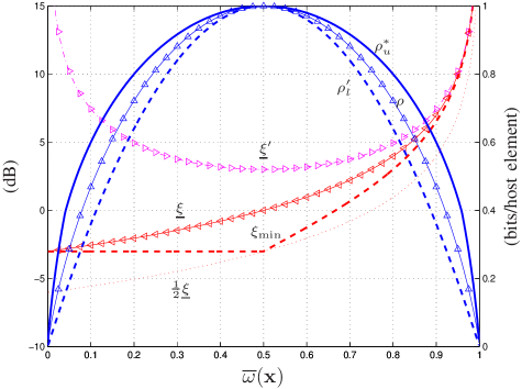
Figure 4: Performance of unpartitioned permutation coding for a host with support $\mathcal{V}=\{0,1\}$ and $n=10^{6}$ as a function of its Hamming weight per symbol. Lines are theoretical results and symbols are empirical measurements. Rate units are on the right-hand side of the plot, whereas distortion units are on the left-hand side; $\rho_{u}^{*}=\min(\rho_{u}^{\prime},\rho_{u}^{\prime\prime})$.

The information-carrying vector $\mathbf{y}=e(\mathbf{x},m)$ is then produced as described in Sections VI and IV-B. In every case it is verified that $\mathbf{y}$ preserves the histogram of $\mathbf{x}$, and that the decoder retrieves the message without error, i.e., $d(\mathbf{y})=m$. The following empirical amounts are computed from $\mathbf{w}=\mathbf{y}-\mathbf{x}$: $\xi_{\textrm{emp}}=\|\mathbf{x}\|^{2}/\|\mathbf{w}\|^{2}$ (empirical host to watermark power ratio), $\xi_{\textrm{emp}}^{\prime}=n(2^{b}-1)^{2}/\|\mathbf{w}\|^{2}$ (empirical peak host to watermark power ratio), $\nu_{\textrm{emp}}=(1/n)\sum_{i=1}^{n}\mathbbold{1}_{\{w_{i}\neq 0\}}$ (empirical degree of host change) and $\varepsilon_{\textrm{emp}}=\rho_{\textrm{emp}}/\nu_{\textrm{emp}}$ bits/host element change (empirical embedding efficiency).

The results in Figure 4 are for unpartitioned permutation coding in the binary Hamming case. As discussed in Section V-E, in this case the asymptotic rate-distortion performance only depends on the normalized Hamming weight of the host, and consequently it is particularly easy to visualize. In the figure, the lower rate-distortion bound is the asymptotic result $\rho_{l}^{\prime}\doteq 2\overline{\nu}$, which is tighter than $\rho_{l}$ because from (27) we have that $\overline{\nu}\leq 1/2$ for a binary host. The upper bound shown is the minimum of (45) and (46). The theoretical rates match the empirical rates accurately, just because $r$ is large and the bounds (67) are asymptotically tight. It is more interesting to see that the empirical distortion results —which correspond to single watermarks (i.e., they are one-shot results and not averages)— accurately match the theoretical predictions involving averages, that is, $\underline{\xi}$ and $\underline{\xi}^{\prime}$. We showed in Section V-A2 that this asymptotic behavior of the embedding distortion of permutation coding for large $n$ is a consequence of the law of large numbers. Also see that, as discussed in Section V-A3, $\xi_{\mathrm{min}}\geq\underline{\xi}/2$.

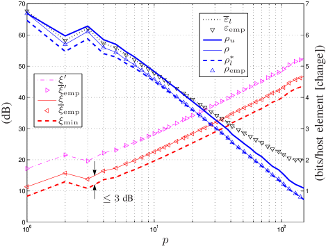
Figure 5: Performance of partitioned permutation coding for a quantized Gaussian host with $n=10^{6}$ as a function of the number of partitions, for the sequence of support partitionings $\{\mathcal{\widetilde{U}}_{q}^{p}\}$. Rate and efficiency units are on the right-hand side of the plot, whereas distortion units are on the left-hand side; $\rho_{l}^{*}=\max(\rho_{l},\rho_{l}^{\prime})$.

We verify next the results for partitioned permutation coding, using a host $\mathbf{x}$ drawn from a Gaussian distribution with mean $128$ and standard deviation $25$, and quantized to $\mathcal{V}=\{0,1,\ldots,2^{b}-1\}$ ($b=8$). The sequence of support partitionings $\{\mathcal{\widetilde{U}}_{q}^{p}\}$ discussed in Section VI-B1 is used to obtain the results in Figure 5. The rate-distortion bound (30) is now key to the achieved performance, whereas (31) is too loose and not shown. Like in the previous figure, we observe a close match between empirical measurements for one-shot experiments and their corresponding averages. This is also true for the match between the empirical embedding efficiency and the lower bound on $\overline{\varepsilon}$. It can be verified that, as discussed in Section VI inequalities (22) and (39) still hold. Finally, the most important feature in Figure 5 is the narrow nearly constant gap $\rho_{u}-\rho_{\text{emp}}$ throughout, which is roughly the same as the gap $\rho_{u}-\rho_{l}^{*}$ between the rate-distortion bounds.

VIII Concluding Remarks

We have given a solution to the fundamental problem of asymptotically optimum perfect universal steganography of finite memoryless sources with a passive warden. We have shown that Slepian’s Variant I permutation codes are central to this problem, and that they can be efficiently implemented by means of adaptive arithmetic coding. This reflects in practice the duality between perfect steganography and lossless compression. We have also studied the embedding distortion of permutation coding, and extended the problem above to include a distortion constraint. The method that we have proposed for the constrained scenario (partitioned permutation coding) performs close to an unattainable upper bound on the rate-distortion function of the problem.

In the same way that optimum lossless source coding of memoryless signals is at the core of compression methods for real-world signals, we expect that optimum perfect steganography of memoryless signals will find its place at the core of future steganographic methods for real-world host signals. Possible approaches include the use of decorrelating integer-to-integer transforms, or decorrelation through predictive techniques such as prediction by partial matching [34], prior to the application of permutation coding. Inevitably, steganography will no longer be perfect when the memoryless assumption becomes only an approximation, but the aforementioned approaches have the virtue of decoupling the steganography problem from the decorrelation problem. To conclude, we should also note that the duality between steganography and source coding also means that the distortion-constrained algorithm we have presented may be of interest in the dual problem of lossless source coding with side information at the decoder (i.e., distributed source coding).

Appendix A Appendix

In this appendix we obtain two expectations of matrix functions of a random variable $\mathit{\Pi}$ uniformly distributed over the ensemble of all permutation matrices, i.e., $\Pr\{\mathit{\Pi}=\Pi_{\boldsymbol{\sigma}}\}=1/n!$ for all ${\boldsymbol{\sigma}}\in\mathcal{S}_{n}$. Firstly, we wish to calculate

$$\mathop{\textrm{E}}\{\mathit{\Pi}\} = \frac{1}{n!}\sum_{\boldsymbol{\sigma}\in\mathcal{S}_{n}}\Pi_{\boldsymbol{\sigma}}.$$ (68)

In order to evaluate (68) consider the number of $n\times n$ permutation matrices which have a one at any given entry. This is equivalent to fixing the corresponding row, and therefore there are $(n-1)!$ possibilities for the remaining $n-1$ rows. Since this holds for any entry, the summation on the right equals $(n-1)!\,\mathbf{1}\mathbf{1}^{t}$, and so we have that

$$\mathop{\textrm{E}}\{\mathit{\Pi}\}=\frac{1}{n}\,\mathbf{1}\mathbf{1}^{t}.$$ (69)

Also see that, if we assume $\Pr\{\mathit{\Pi}=\Pi_{\boldsymbol{\sigma}}\}=1/r$ for all ${\boldsymbol{\sigma}}\in\mathcal{S}_{\mathbf{x}}$, then the average vector $\mathop{\textrm{E}}\{\mathit{\Pi}\mathbf{x}\}$ can be obtained using (69) by observing that

$$\frac{1}{r}\sum_{\boldsymbol{\sigma}\in\mathcal{S}_{\mathbf{x}}}\Pi_{\boldsymbol{\sigma}}\mathbf{x}=\frac{1}{n!}\sum_{\boldsymbol{\sigma}\in\mathcal{S}_{n}}\Pi_{\boldsymbol{\sigma}}\mathbf{x},$$ (70)

which holds because the second sum contains the same summands as the first one, but each repeated $h_{1}!h_{2}!\cdots h_{q}!$ times.

Next we wish to compute

$$\mathop{\textrm{E}}\left\{\mathit{\Pi}\mathbf{x}\mathbf{x}^{t}\mathit{\Pi}^{t}\right\} = \frac{1}{n!}\sum_{\boldsymbol{\sigma}\in\mathcal{S}_{n}}\Pi_{\boldsymbol{\sigma}}\mathbf{x}\mathbf{x}^{t}\Pi_{\boldsymbol{\sigma}}^{t},$$ (71)

for some arbitrary vector $\mathbf{x}$. This average is a particular case of the general formula given by Daniels in [35, equation (4.9)]:

$$\mathop{\textrm{E}}\left\{\mathit{\Pi}\mathbf{x}\mathbf{x}^{t}\mathit{\Pi}^{t}\right\}=a\,\mathrm{I}+b\,\mathbf{1}\mathbf{1}^{t},$$

with $b=\left((\mathbf{x}^{t}\mathbf{1})^{2}-\|\mathbf{x}\|^{2}\right)/(n(n-1))$ and $a+b=(1/n)\|\mathbf{x}\|^{2}$.

Finally observe that average (71) is the same if we replace $n!$ and $\mathcal{S}_{n}$ by $r$ and $\mathcal{S}_{\mathbf{x}}$, for the same reason that makes expression (70) true.

Félix Balado (M’03) graduated with an M.Eng. in Telecommunications Engineering from the University of Vigo (Spain) in 1996, and received a Ph.D. from the same institution in 2003 for his work in digital data hiding. He is currently a lecturer in University College Dublin (Ireland). His research interests lie in the areas of signal processing, digital communications, and bioinformatics.

David Haughton received a Ph.D. from University College Dublin (Ireland) in 2014, for his work in the area of information embedding in DNA. He is currently a senior data scientist in the Centre for Applied Data Analytics Research in Dublin (Ireland). His research background is in signal processing, bioinformatics and steganography, and his current research interest lies in big data analytics.

References

- [1] P. Moulin and R. Koetter, “Data-hiding codes,” Proc. IEEE, vol. 93, pp. 2083–2127, December 2005.
- [2] R. Anderson and F. Petitcolas, “On the limits of steganography,” IEEE J. Select. Areas Commun., vol. 4, pp. 474–481, May 1998.
- [3] C. Cachin, “An information-theoretic model for steganography,” in Procs. of the 2nd Int. Workshop on Information Hiding, ser. LNCS, vol. 1525. Portland, USA: Springer-Verlag, April 1998, pp. 306–318.
- [4] P. Sallee, “Model-based steganography,” in Procs. of the 2nd Int. Workshop on Digital Watermarking (IWDW), Seoul, Korea, October 2003, pp. 154–167.
- [5] P. Comesaña and F. Pérez-González, “On the capacity of stegosystems,” in Procs. of the 9th ACM Workshop on Multimedia & Security, Dallas, USA, September 2007, pp. 15–24.
- [6] Y. Wang and P. Moulin, “Perfectly secure steganography: Capacity, error exponents, and code constructions,” IEEE Trans. on Inf. Theory, vol. 54, no. 6, pp. 2706–2722, June 2008.
- [7] D. Slepian, “Permutation modulation,” Procs. of the IEEE, vol. 53, no. 3, pp. 228–236, Mar. 1965.
- [8] B. Ryabko and D. Ryabko, “Asymptotically optimal perfect steganographic systems,” Problems of Information Transmission, vol. 45, no. 2, pp. 184–190, February 2009.
- [9] S. Verdú, “Teaching lossless data compression,” IEEE Information Theory Society Newsletter, vol. 61, no. 1, pp. 18–19, April 2011.
- [10] M. H. Costa, “Writing on dirty paper,” IEEE Trans. on Information Theory, vol. 29, no. 3, pp. 439–441, May 1983.
- [11] N. Provos, “Defending against statistical steganalysis,” in Procs. of the 10th USENIX Security Symposium, Washington D.C., USA, August 2001, pp. 323–335.
- [12] E. Franz, “Steganography preserving statistical properties,” in Information Hiding, ser. Lecture Notes in Computer Science, F. Petitcolas, Ed. Springer, 2003, vol. 2578, pp. 278–294.
- [13] M. Kumar and R. Newman, “J3: High payload histogram neutral JPEG steganography,” in 8th Annual Int. Conf. on Privacy, Security and Trust (PST), Otawa, Canada, August 2010, pp. 46–53.
- [14] G. Luo and K. Subbalakshmi, “Zero Kullback-Leibler divergence image data hiding,” in IEEE Global Telecommunications Conf. (GLOBECOM), Houston, USA, December 2011, pp. 1–5.
- [15] B. Ryabko, “Fast enumeration of combinatorial objects,” Diskretnaya Mathematika, vol. 10, no. 2, pp. 101–119, 1998.
- [16] T. Mittelholzer, “An information-theoretic approach to steganography and watermarking,” in Procs. of the 3rd Int. Information Hiding Workshop, ser. LNCS, vol. 1768. Dresden, Germany: Springer-Verlag, October 1999, pp. 1–16.
- [17] T. Berger, F. Jelinek, and J. Wolf, “Permutation codes for sources,” IEEE Trans. Inf. Theory, vol. 18, no. 1, pp. 160–169, Jan. 1972.
- [18] T. M. Cover and J. A. Thomas, Elements of Information Theory, 2nd ed. John Wiley & Sons, 2006.
- [19] R. C. Pasco, “Source coding algorithms for fast data compression,” Ph.D. dissertation, Stanford University, May 1976.
- [20] J. Rissanen, “Generalized Kraft inequality and arithmetic coding,” IBM J. Res. Dev., vol. 20, no. 198, 1976.
- [21] J. Cleary and I. Witten, “A comparison of enumerative and adaptive codes,” IEEE Trans. Inf. Theory, vol. 30, no. 2, pp. 306–315, March 1984.
- [22] J. Rissanen, “Arithmetic codings as number representations,” Acta Polytech. Scand. Math, vol. 31, pp. 44–51, Dec. 1979.
- [23] G. H. Hardy, J. E. Littlewood, and G. Pólya, Inequalities. Cambridge, at the University Press, 1934.
- [24] A. G. Djackov, “On a search model of false coins,” in Topics in Information Theory, ser. Colloquia Mathematica Societatis János Bolyai, I. Csiszár and P. Elias, Eds. Budapest, Hungary: North Holland Publishing Co., 1977, vol. 16, pp. 163–170.
- [25] J. L. Massey, “On the entropy of integer-valued random variables,” in Procs. of Int. Workshop on Information Theory, Beijing, China, July 1988, pp. C1.2–C1.4.
- [26] P. Harremoës and F. Topsøe, “Inequalities between entropy and index of coincidence derived from information diagrams,” IEEE Trans. Inf. Theory, vol. 47, no. 7, pp. 2944–2960, November 2001.
- [27] A. Westfeld, “F5 – A steganographic algorithm,” in Procs. of the 4th Int. Information Hiding Workshop, ser. LNCS, vol. 2137. Springer-Verlag, 2001, pp. 289–302.
- [28] P. Montmort, Essay d’Analyse sur les Jeux de Hazard, Paris, 1708.
- [29] G. Cohen, “A nonconstructive upper bound on covering radius,” IEEE Trans. on Information Theory, vol. 29, no. 3, pp. 352–353, May 1983.
- [30] T. Sharp, “An implementation of key-based digital signal steganography,” in Procs. of the 4th Information Hiding Workshop, ser. LNCS, vol. 2137. Springer-Verlag, 2001, pp. 13–26.
- [31] S. I. Gel’fand and M. S. Pinsker, “Coding for channel with random parameters,” Problems of Control and Information Theory, vol. 9, no. 1, pp. 19–31, 1980.
- [32] R. J. Barron, B. Chen, and G. W. Wornell, “The duality between information embedding and source coding with side information and some applications,” IEEE Trans. Inf. Theory, vol. 49, no. 5, pp. 1159–1180, May 2003.
- [33] H. Robbins, “A remark on Stirling’s formula,” The American Mathematical Monthly, vol. 62, no. 1, pp. 26–29, January 1955.
- [34] J. Cleary and I. Witten, “Data compression using adaptive coding and partial string matching,” IEEE Trans. Commun., vol. 32, no. 4, pp. 396–402, Apr 1984.
- [35] H. E. Daniels, “Processes generating permutation expansions,” Biometrika, vol. 49, no. 1/2, pp. 139–149, June 1962.