Equilibration of a quantum field in de Sitter space-time

Andreas Albrecht ajalbrecht@ucdavis.edu University of California at Davis, Department of Physics, One Shields Ave, Davis CA 95616 USA    R. Holman rh4a@andrew.cmu.edu Physics Department, Carnegie Mellon University, Pittsburgh PA 15213 USA    Benoit J. Richard bjrichard@ucdavis.edu University of California at Davis, Department of Physics, One Shields Avenue, Davis CA 95616 USA
Abstract

We address the following question: To what extent can a quantum field tell if it has been placed in de Sitter space? Our approach is to use the techniques of non-equilibrium quantum field theory to compute the time evolution of a state which starts off in flat space for (conformal) times η<η0𝜂subscript𝜂0\eta<\eta_{0}, and then evolves in a de Sitter background turned on instantaneously at η=η0𝜂subscript𝜂0\eta=\eta_{0}. We find that the answer depends on what quantities one examines. We study a range of them, all based on two-point correlation functions, and analyze which ones approach the standard Bunch-Davies values over time. The outcome of this analysis suggests that the nature of the equilibration process in this system is similar to that in more familiar systems.

pacs:
98.80.Qc, 11.25.Wx

I Introduction

De Sitter space is widely accepted as a probable early-universe cosmological solution, as it describes the state of the universe during inflation. Provided our universe possesses a completely stable positive cosmological constant, it should also asymptotically approach de Sitter space at late times111Such an idea is at the heart of de Sitter Equilibrium, an alternative to eternal inflation as an initial conditions independent cosmological framework Albrecht and Sorbo (2004); Albrecht (2009), but the motivation for this paper is broader than this..

The standard lore of de Sitter space is that it acts as a heat bath, in such a way that an Unruh-deWitt detector for a quantum field in a de Sitter background will register a thermal spectrum for the number of particles in a given momentum mode (Birrell and Davies (1982) and references therein). But how does this happen? If de Sitter space is past and future eternal and the state is de Sitter invariant, then it should not come as a surprise that the Green’s functions of the quantum field embedded in this background should partake of its thermal behavior as evidenced by the periodicity in imaginary time inherent in the metric Gibbons and Hawking (1977). However, suppose we start the de Sitter evolution at an initial time, as might happen in inflation, say, and further assume that we start the field in a state that is not de Sitter invariant. What happens next?

We address this question here in a particular scheme which is chosen to be relevant to the question and also technically tractable. Consider the situation where, for conformal times η<η0𝜂subscript𝜂0\eta<\eta_{0}, the background geometry is that of Minkowski flat space-time, and a minimally coupled free field is taken to be in the free field vacuum state of the flat space Hamiltonian. Then at η=η0𝜂subscript𝜂0\eta=\eta_{0}, the background is changed to become de Sitter space with an expansion rate H𝐻H so that the Gibbons-Hawking temperature is TdeS=H2πsubscript𝑇deS𝐻2𝜋T_{\rm de\ S}=\frac{H}{2\pi}. Since we are only considering free field theory in a time-dependent background, we can solve the functional Schrödinger equation for the wave functional describing the state of the field explicitly, and use this wave functional to understand to what extent does this state approximate the “thermal” Bunch-Davies (BD) state Bunch and Davies (1978) (extending the work on the corresponding modes by Schomblond and Spindel Schomblond and Spindel (1976)), by analyzing ratios of various correlators and momentum-energy tensors, evaluated in our vacuum state to the quantities considered in the BD vacuum state.

This issue is not only of conceptual relevance, but could have observational consequences as well. The state of the field prior to inflation need not be one that matches on smoothly to the BD state at the onset of inflation, and if the number of e-folds is close to the minimum it is not an outlandish thought that some remnants of this pre-inflationary state might have survived to imprint themselves on the CMB and/or large scale structure. Conversely, given how well the power spectrum of CMB fluctuations has been measured Bennett et al. (2012); Ade et al (2013), and how closely this spectrum follows what would have been expected from the assumptions of an initial BD state, we can use this data and our calculation to constrain the space of allowed initial states for inflationary fluctuations.

It is worth noting that the question we are asking can be recast as: to what extent are there no-hair theorems for the quantum state of a test field in de Sitter space? There has been some prior work in this direction, starting from the seminal work of Ford and Vilenkin Vilenkin and Ford (1982) as well as the more recent one of Anderson, Eaker, Habib, and Molina-París Anderson et al. (2000). In both cases, an attractor behavior was found for sufficiently well-behaved states. Related issues were also addressed in Fischler et al. (2014a), Fischler et al. (2014b), Singh et al. (2013a), and Singh et al. (2013b). Our viewpoint is somewhat different here; we don’t know what the state of the field is prior to inflation but, regardless, it should be reasonable to ask what the evolution of that state is after inflation begins. Then we can ask to what extent the BD behavior is generic at late times during inflation.

In the next section we set up the initial value problem for the Schrödinger wave functional with the flat space initial conditions described above. We then use that wave functional to compute two-point functions in our state. Since we have a free field theory, that state will be a gaussian, and thus fully described by the three correlation functions: ΦkΦkdelimited-⟨⟩subscriptΦ𝑘subscriptΦ𝑘\langle\Phi_{\vec{k}}\Phi_{-\vec{k}}\rangle, ΠkΠkdelimited-⟨⟩subscriptΠ𝑘subscriptΠ𝑘\langle\Pi_{\vec{k}}\Pi_{-\vec{k}}\rangle, and ΠkΦk+ΦkΠkdelimited-⟨⟩subscriptΠ𝑘subscriptΦ𝑘subscriptΦ𝑘subscriptΠ𝑘\langle\Pi_{\vec{k}}\Phi_{-\vec{k}}+\Phi_{\vec{k}}\Pi_{-\vec{k}}\rangle. Additionally, we study observables such as the expectation value of the stress-energy tensor of this state. Section III is devoted to numerical results and the analysis of ratios of two-point functions, and stress-energy tensors, evaluated in both our state and the BD states. We end with a discussion of our results as well as some further directions to take in addressing the issues dealt with here. Overall our vacuum state approaches the BD state, when considering coarse-grained collections of modes clearly within the horizon.

II Wave Functional, Mode Equation, and Correlation Functions

II.1 Finding the Schrödinger wave functional

As discussed in the introduction, we consider a test scalar field embedded in an FRW space-time that transitions between a constant scale factor for conformal times ηη0𝜂subscript𝜂0\eta\leq\eta_{0} to a de Sitter scale factor for η>η0𝜂subscript𝜂0\eta>\eta_{0}. We assume that such a space-time is generated by an appropriate stress-energy tensor via the Einstein equations, but do not concern ourselves further with how this background geometry is obtained.

If Φ(x,η)Φ𝑥𝜂\Phi(\vec{x},\eta) denotes the scalar field in question, the action we use is

S=12d4xa4(η)[1a2(η)(Φ2(Φ)2)m2Φ2],𝑆12superscript𝑑4𝑥superscript𝑎4𝜂delimited-[]1superscript𝑎2𝜂superscriptΦ2superscriptΦ2superscript𝑚2superscriptΦ2S=\frac{1}{2}\int d^{4}xa^{4}(\eta)\left[\frac{1}{a^{2}(\eta)}\left(\Phi^{\prime 2}-(\nabla\Phi)^{2}\right)-m^{2}\Phi^{2}\right], (1)

where a prime denotes a derivative with respect to η𝜂\eta, and m2=mΦ2+ξBRsuperscript𝑚2subscriptsuperscript𝑚2Φsubscript𝜉𝐵𝑅m^{2}=m^{2}_{\Phi}+\xi_{B}R, mΦsubscript𝑚Φm_{\Phi} referring to the mass of our field. We will take the scale factor as

a(η)={1η0Hηη01ηHη>η0𝑎𝜂cases1subscript𝜂0𝐻𝜂subscript𝜂01𝜂𝐻𝜂subscript𝜂0a(\eta)=\left\{\begin{array}[]{cc}-\frac{1}{\eta_{0}H}&\eta\leq\eta_{0}\\ -\frac{1}{\eta H}&\eta>\eta_{0}\end{array}\right. (2)

The scale factor is continuous though not differentiable at η=η0𝜂subscript𝜂0\eta=\eta_{0}. A more reasonable assumption would be that the transition is smoother than this (for an example see Vilenkin and Ford (1982)), but this will suffice for our purposes.

Instead of quantizing this theory in the usual way (i.e., by defining creation and annihilation operators acting on the Fock space of states) we will use a Schrödinger picture quantization Boyanovsky et al. (1994). Here we use eigenstates of the Schrödinger picture field operator Φ^(x)^Φ𝑥\hat{\Phi}(\vec{x}), |Φ()ketΦ|\Phi(\cdot)\rangle such that

Φ^(x)|Φ()=Φ(x)|Φ().^Φ𝑥ketΦΦ𝑥ketΦ\hat{\Phi}(\vec{x})|\Phi(\cdot)\rangle=\Phi(\vec{x})|\Phi(\cdot)\rangle. (3)

The state of the field is then represented by a wave functional Ψ[Φ();η]ΨΦ𝜂\Psi\left[\Phi(\cdot);\eta\right] (or more generally by a density matrix element ρ[Φ(),Φ~();η]𝜌Φ~Φ𝜂\rho[\Phi(\cdot),\tilde{\Phi}(\cdot);\eta]) satisfying the Schrödinger (Liouville) equation

iΨ[Φ();η]η=H^[iδδΦ(),Φ()]Ψ[Φ();η](or iρη=[H^,ρ]),𝑖ΨΦ𝜂𝜂^𝐻𝑖𝛿𝛿ΦΦΨΦ𝜂or 𝑖𝜌𝜂^𝐻𝜌i\frac{\partial\Psi[\Phi(\cdot);\eta]}{\partial\eta}=\hat{H}\left[-i\frac{\delta}{\delta\Phi(\cdot)},\Phi(\cdot)\right]\Psi[\Phi(\cdot);\eta]\quad\left(\text{or }i\frac{\partial\rho}{\partial\eta}=\left[\hat{H},\rho\right]\right), (4)

where H^^𝐻\hat{H} is the Hamiltonian operator (again in the Schrödinger picture) obtained from the action in Eq. (1). For our case this reads

H^=d3x{Π22a2(η)+12a2(η)(Φ(x))2+12m2a4(η)Φ(x)2},^𝐻superscript𝑑3𝑥superscriptΠ22superscript𝑎2𝜂12superscript𝑎2𝜂superscriptΦ𝑥212superscript𝑚2superscript𝑎4𝜂Φsuperscript𝑥2\hat{H}=\int d^{3}x\left\{\frac{\Pi^{2}}{2a^{2}(\eta)}+\frac{1}{2}a^{2}(\eta)\left(\nabla\Phi(\vec{x})\right)^{2}+\frac{1}{2}m^{2}a^{4}(\eta)\Phi(\vec{x})^{2}\right\}, (5)

with Π=a2(η)ΦΠsuperscript𝑎2𝜂superscriptΦ\Pi=a^{2}(\eta)\Phi^{\prime} being the canonically conjugate momentum to ΦΦ\Phi, represented in the usual way as Πiδ/δΦ()Π𝑖𝛿𝛿Φ\Pi\rightarrow-i\delta/\delta\Phi(\cdot) in the Schrödinger picture.

We note that the Schrödinger equation in Eq. (4) should be written using the proper time of the observer measuring the wave function. For an FRW space-time this would be the cosmic time t𝑡t. However, the use of conformal time corresponds to a canonical transformation and thus gives rise to the same physics Boyanovsky et al. (1994), as would be expected of a coordinate transformation. It will be important in our later analysis to keep in mind that t𝑡t\rightarrow\infty corresponds to η0𝜂superscript0\eta\rightarrow 0^{-}.

We will take our spatial geometry to be flat so we can expand the field in terms of Fourier components. Furthermore, we will quantize our field in a box of comoving spatial volume V𝑉V so that the Schrödinger picture field and conjugate momenta can be written as

Φ(x)=1VkΦkeikxΦ𝑥1𝑉subscript𝑘subscriptΦ𝑘superscript𝑒𝑖𝑘𝑥\displaystyle\Phi(\vec{x})=\frac{1}{\sqrt{V}}\sum_{\vec{k}}\Phi_{\vec{k}}e^{-i\vec{k}\cdot\vec{x}}
Π(x)=1VkΠkeikx,Π𝑥1𝑉subscript𝑘subscriptΠ𝑘superscript𝑒𝑖𝑘𝑥\displaystyle\Pi(\vec{x})=\frac{1}{\sqrt{V}}\sum_{\vec{k}}\Pi_{\vec{k}}e^{-i\vec{k}\cdot\vec{x}}, (6)

where the equal time commutation relations

[ΦS(x),ΠS(y)]=iδ3(xy)subscriptΦ𝑆𝑥subscriptΠ𝑆𝑦𝑖superscript𝛿3𝑥𝑦\left[\Phi_{S}(\vec{x}),\Pi_{S}(\vec{y})\right]=i\delta^{3}(\vec{x}-\vec{y}) (7)

imply [Φk,Πq]=iδk,qsubscriptΦ𝑘subscriptΠ𝑞𝑖subscript𝛿𝑘𝑞\left[\Phi_{\vec{k}},\Pi_{\vec{q}}\right]=i\delta_{\vec{k},-\vec{q}} and thus, in the Schrödinger picture, ΠqsubscriptΠ𝑞\Pi_{\vec{q}} can be represented as iδδΦq𝑖𝛿𝛿subscriptΦ𝑞-i\frac{\delta}{\delta\Phi_{\vec{-q}}}. Hence, the Hamiltonian breaks up into the sum of Hamiltonians for each mode, and we can also write the wave function as the product of wave functions for each mode:

H=kHkwith Hk=ΠkΠk2a2(η)+12a2(η)Ωk2(η)ΦkΦk,formulae-sequence𝐻subscript𝑘subscript𝐻𝑘with subscript𝐻𝑘subscriptΠ𝑘subscriptΠ𝑘2superscript𝑎2𝜂12superscript𝑎2𝜂superscriptsubscriptΩ𝑘2𝜂subscriptΦ𝑘subscriptΦ𝑘\displaystyle H=\sum_{\vec{k}}H_{\vec{k}}\quad\text{with }H_{\vec{k}}=\frac{\Pi_{\vec{k}}\Pi_{-\vec{k}}}{2a^{2}(\eta)}+\frac{1}{2}a^{2}(\eta)\Omega_{\vec{k}}^{2}(\eta)\ \Phi_{\vec{k}}\Phi_{-\vec{k}},
Ψ[{Φk},η]=kψk(Φk,η),ΨsubscriptΦ𝑘𝜂subscriptproduct𝑘subscript𝜓𝑘subscriptΦ𝑘𝜂\displaystyle\Psi[\{\Phi_{\vec{k}}\},\eta]=\prod_{\vec{k}}\psi_{\vec{k}}(\Phi_{\vec{k}},\eta),
Ωk2(η)k2+m2a2(η).superscriptsubscriptΩ𝑘2𝜂superscript𝑘2superscript𝑚2superscript𝑎2𝜂\displaystyle\Omega_{k}^{2}(\eta)\equiv k^{2}+m^{2}a^{2}(\eta). (8)

Since we have a free field theory, our ansatz for the ground-state wave functional for each mode should be Gaussian as in

ψk(Φk,η)=Nk(η)exp(12Ak(η)ΦkΦk),subscript𝜓𝑘subscriptΦ𝑘𝜂subscript𝑁𝑘𝜂12subscript𝐴𝑘𝜂subscriptΦ𝑘subscriptΦ𝑘\psi_{\vec{k}}(\Phi_{\vec{k}},\eta)=N_{\vec{k}}(\eta)\exp\left(-\frac{1}{2}A_{k}(\eta)\Phi_{\vec{k}}\Phi_{-\vec{k}}\right), (9)

where we have made use of rotational invariance to write the kernel Ak(η)subscript𝐴𝑘𝜂A_{k}(\eta) as a function of the magnitude k𝑘k of k𝑘\vec{k}. By matching powers of ΦksubscriptΦ𝑘\Phi_{\vec{k}} on either side of the Schrödinger equation for each mode we find:

iNk(η)Nk(η)=Ak(η)2a2(η)𝑖superscriptsubscript𝑁𝑘𝜂subscript𝑁𝑘𝜂subscript𝐴𝑘𝜂2superscript𝑎2𝜂\displaystyle i\frac{N_{\vec{k}}^{\prime}(\eta)}{N_{\vec{k}}(\eta)}=\frac{A_{k}(\eta)}{2a^{2}(\eta)} (10)
iAk(η)=Ak2(η)a2(η)a2(η)Ωk2(η)Ak(η0)=Ωk(η0)a2(η0)formulae-sequence𝑖superscriptsubscript𝐴𝑘𝜂superscriptsubscript𝐴𝑘2𝜂superscript𝑎2𝜂superscript𝑎2𝜂superscriptsubscriptΩ𝑘2𝜂subscript𝐴𝑘subscript𝜂0subscriptΩ𝑘subscript𝜂0superscript𝑎2subscript𝜂0\displaystyle iA_{k}^{\prime}(\eta)=\frac{A_{k}^{2}(\eta)}{a^{2}(\eta)}-a^{2}(\eta)\Omega_{k}^{2}(\eta)\quad A_{k}(\eta_{0})=\Omega_{k}(\eta_{0})a^{2}(\eta_{0})

where the primes represent conformal time derivatives, and the initial condition is found by considering the ground state wave function of a quantum mechanical harmonic oscillator with mass a2(η0)superscript𝑎2subscript𝜂0a^{2}(\eta_{0}) and frequency Ωk(η0)subscriptΩ𝑘subscript𝜂0\Omega_{k}(\eta_{0}).

II.2 Solving the mode equations

Eq. (10) is of the Ricatti form and can be converted into a second order equation of Schrödinger type via the substitution

Ak(η)=ia2(η)(ϕk(η)ϕk(η)a(η)a(η)).subscript𝐴𝑘𝜂𝑖superscript𝑎2𝜂superscriptsubscriptitalic-ϕ𝑘𝜂subscriptitalic-ϕ𝑘𝜂superscript𝑎𝜂𝑎𝜂A_{k}(\eta)=-ia^{2}(\eta)\left(\frac{\phi_{k}^{\prime}(\eta)}{\phi_{k}(\eta)}-\frac{a^{\prime}(\eta)}{a(\eta)}\right). (11)

Doing this we find

ϕk′′(η)+(Ωk2(η)a′′(η)a(η))ϕk(η)=0,ϕk(η0)=(iΩk(η0)+a(η0)a(η0))ϕk(η0).formulae-sequencesuperscriptsubscriptitalic-ϕ𝑘′′𝜂superscriptsubscriptΩ𝑘2𝜂superscript𝑎′′𝜂𝑎𝜂subscriptitalic-ϕ𝑘𝜂0superscriptsubscriptitalic-ϕ𝑘subscript𝜂0𝑖subscriptΩ𝑘subscript𝜂0superscript𝑎subscript𝜂0𝑎subscript𝜂0subscriptitalic-ϕ𝑘subscript𝜂0\phi_{k}^{\prime\prime}(\eta)+\left(\Omega_{k}^{2}(\eta)-\frac{a^{\prime\prime}(\eta)}{a(\eta)}\right)\phi_{k}(\eta)=0,\quad\phi_{k}^{\prime}(\eta_{0})=\left(i\Omega_{k}(\eta_{0})+\frac{a^{\prime}(\eta_{0})}{a(\eta_{0})}\right)\phi_{k}(\eta_{0}). (12)

The equation we start with for Ak(η)subscript𝐴𝑘𝜂A_{k}(\eta) is a first order equation and we have one initial condition for it so that there is a unique solution for Ak(η)subscript𝐴𝑘𝜂A_{k}(\eta). On the other hand, the equation for ϕk(η)subscriptitalic-ϕ𝑘𝜂\phi_{k}(\eta) is a second order one, requiring two initial conditions for a unique solution. The resolution of this dilemma can be found by noting that Aksubscript𝐴𝑘A_{k} is related to the ratio of ϕksuperscriptsubscriptitalic-ϕ𝑘\phi_{k}^{\prime} and ϕksubscriptitalic-ϕ𝑘\phi_{k}. This means that in any linear combination of the two independent solutions to Eq. (12), we can factor out an overall constant leaving only one constant to be determined. We can use this freedom to fix the (constant) Wronskian of ϕk(η)subscriptitalic-ϕ𝑘𝜂\phi_{k}(\eta) and ϕk(η)superscriptsubscriptitalic-ϕ𝑘𝜂\phi_{k}^{*}(\eta) to equal i𝑖-i. Imposing this condition then implies that ϕk(η0)=12Ωk(η0)subscriptitalic-ϕ𝑘subscript𝜂012subscriptΩ𝑘subscript𝜂0\phi_{k}(\eta_{0})=\frac{1}{\sqrt{2\Omega_{k}(\eta_{0})}}.

Eq. (12) is nothing but the mode equation for a massive, minimally coupled scalar field in de Sitter space. The solutions are well known Schomblond and Spindel (1976) and we can write

ϕk(η)=αk𝒰k(η)+βk𝒰k(η),𝒰k(η)=πη2Hν(2)(kη),formulae-sequencesubscriptitalic-ϕ𝑘𝜂subscript𝛼𝑘subscript𝒰𝑘𝜂subscript𝛽𝑘superscriptsubscript𝒰𝑘𝜂subscript𝒰𝑘𝜂𝜋𝜂2superscriptsubscript𝐻𝜈2𝑘𝜂\displaystyle\phi_{k}(\eta)=\alpha_{k}{\cal U}_{k}(\eta)+\beta_{k}{\cal U}_{k}^{*}(\eta),\quad{\cal U}_{k}(\eta)=\frac{\sqrt{-\pi\eta}}{2}H_{\nu}^{(2)}(-k\eta),
αk=i2Ωk(η0)[𝒰k(η0)+(iΩk(η0)+1η0)𝒰k(η0)],subscript𝛼𝑘𝑖2subscriptΩ𝑘subscript𝜂0delimited-[]superscriptsubscript𝒰𝑘subscript𝜂0𝑖subscriptΩ𝑘subscript𝜂01subscript𝜂0superscriptsubscript𝒰𝑘subscript𝜂0\displaystyle\alpha_{k}=\frac{i}{\sqrt{2\Omega_{k}(\eta_{0})}}\left[{\cal U}_{k}^{*\prime}(\eta_{0})+\left(-i\Omega_{k}(\eta_{0})+\frac{1}{\eta_{0}}\right){\cal U}_{k}^{*}(\eta_{0})\right], (13)
βk=i2Ωk(η0)[𝒰k(η0)+(iΩk(η0)+1η0)𝒰k(η0)],subscript𝛽𝑘𝑖2subscriptΩ𝑘subscript𝜂0delimited-[]superscriptsubscript𝒰𝑘subscript𝜂0𝑖subscriptΩ𝑘subscript𝜂01subscript𝜂0subscript𝒰𝑘subscript𝜂0\displaystyle\beta_{k}=-\frac{i}{\sqrt{2\Omega_{k}(\eta_{0})}}\left[{\cal U}_{k}^{\prime}(\eta_{0})+\left(-i\Omega_{k}(\eta_{0})+\frac{1}{\eta_{0}}\right){\cal U}_{k}(\eta_{0})\right],

where ν=94m2H2𝜈94superscript𝑚2superscript𝐻2\nu=\sqrt{\frac{9}{4}-\frac{m^{2}}{H^{2}}} and 𝒰k(η)subscript𝒰𝑘𝜂{\cal U}_{k}(\eta) is commonly referred to as the kthsuperscript𝑘𝑡k^{th} Bunch-Davies mode. It is easy to check that the Wronskian condition implies that |αk|2|βk|2=1superscriptsubscript𝛼𝑘2superscriptsubscript𝛽𝑘21|\alpha_{k}|^{2}-|\beta_{k}|^{2}=1; had we been doing Heisenberg field theory, we would infer that the modes ϕk(η)subscriptitalic-ϕ𝑘𝜂\phi_{k}(\eta) are just the Bogoliubov transforms of the BD modes. Moreover, as η0subscript𝜂0\eta_{0}\rightarrow-\infty, the form of 𝒰k(η)subscript𝒰𝑘𝜂{\cal U}_{k}(\eta) allows us to conclude:

Ωk(η0)ksubscriptΩ𝑘subscript𝜂0𝑘\displaystyle\Omega_{k}(\eta_{0})\rightarrow k
𝒰k(η0)12k,subscript𝒰𝑘subscript𝜂012𝑘\displaystyle{\cal U}_{k}(\eta_{0})\rightarrow\frac{1}{\sqrt{2k}}, (14)
𝒰k(η0)ik2,subscriptsuperscript𝒰𝑘subscript𝜂0𝑖𝑘2\displaystyle{\cal U^{\prime}}_{k}(\eta_{0})\rightarrow i\sqrt{\frac{k}{2}},

from which we can infer αk1subscript𝛼𝑘1\alpha_{k}\rightarrow 1 and βk0subscript𝛽𝑘0\beta_{k}\rightarrow 0, i.e. in this limit, we go back to an eternal inflationary patch of de Sitter space with the field state being the BD state.

The full wave function for the mode ΦksubscriptΦ𝑘\Phi_{\vec{k}} is thus given by

ψk(η)=(a2(η)π|ϕk(η)|2)14exp[i2a2(η)(ϕk(η)ϕk(η)a(η)a(η))ΦkΦk],subscript𝜓𝑘𝜂superscriptsuperscript𝑎2𝜂𝜋superscriptsubscriptitalic-ϕ𝑘𝜂214𝑖2superscript𝑎2𝜂superscriptsubscriptitalic-ϕ𝑘𝜂subscriptitalic-ϕ𝑘𝜂superscript𝑎𝜂𝑎𝜂subscriptΦ𝑘subscriptΦ𝑘\psi_{\vec{k}}(\eta)=\left(\frac{a^{2}(\eta)}{\pi\left|\phi_{k}(\eta)\right|^{2}}\right)^{\frac{1}{4}}\exp\left[\frac{i}{2}a^{2}(\eta)\left(\frac{\phi_{k}^{\prime}(\eta)}{\phi_{k}(\eta)}-\frac{a^{\prime}(\eta)}{a(\eta)}\right)\Phi_{\vec{k}}\Phi_{-\vec{k}}\right], (15)

where we should note that when computing any expectation values for quantities involving the mode ΦksubscriptΦ𝑘\Phi_{\vec{k}}, we also need to include the contribution of the wave function ψk(η)subscript𝜓𝑘𝜂\psi_{-\vec{k}}(\eta), since Φk=ΦksubscriptΦ𝑘superscriptsubscriptΦ𝑘\Phi_{-\vec{k}}=\Phi_{\vec{k}}^{*}, and ΦΦ\Phi is a real field. This is equivalent to using the square of ψk(η)subscript𝜓𝑘𝜂\psi_{\vec{k}}(\eta) in any such calculation.

Eq. (15) coupled with the mode equations (12) gives the full specification of the quantum state with the given initial conditions. We can now use this wave function to compute observables that might help us answer the question asked in the introduction: to what extent does this state “feel” de Sitter space?

II.3 Calculating relevant correlation functions

What are the useful diagnostic tools to evaluate the behavior of this state? Since the state is Gaussian, it can be fully specified by the following correlators: ΦkΦk,ΠkΠk,ΠkΦk+ΦkΠkdelimited-⟨⟩subscriptΦ𝑘subscriptΦ𝑘delimited-⟨⟩subscriptΠ𝑘subscriptΠ𝑘delimited-⟨⟩subscriptΠ𝑘subscriptΦ𝑘subscriptΦ𝑘subscriptΠ𝑘\langle\Phi_{\vec{k}}\Phi_{-\vec{k}}\rangle,\ \langle\Pi_{\vec{k}}\Pi_{-\vec{k}}\rangle,\ \langle\Pi_{\vec{k}}\Phi_{-\vec{k}}+\Phi_{\vec{k}}\Pi_{-\vec{k}}\rangle, computed below.

From (15) computing ΦkΦk(η)delimited-⟨⟩subscriptΦ𝑘subscriptΦ𝑘𝜂\langle\Phi_{\vec{k}}\Phi_{-\vec{k}}\rangle(\eta) results in

ΦkΦk(η)delimited-⟨⟩subscriptΦ𝑘subscriptΦ𝑘𝜂\displaystyle\langle\Phi_{\vec{k}}\Phi_{-\vec{k}}\rangle(\eta) =𝒟Φk|ψk(η)|2|ψk(η)|2ΦkΦkabsent𝒟subscriptΦ𝑘superscriptsubscript𝜓𝑘𝜂2superscriptsubscript𝜓𝑘𝜂2subscriptΦ𝑘subscriptΦ𝑘\displaystyle=\int{\cal D}\Phi_{\vec{k}}\left|\psi_{\vec{k}}(\eta)\right|^{2}\left|\psi_{-\vec{k}}(\eta)\right|^{2}\Phi_{\vec{k}}\Phi_{-\vec{k}}
=12AkRabsent12subscript𝐴𝑘𝑅\displaystyle=\frac{1}{2A_{kR}}
=|ϕk(η)|2a2(η).absentsuperscriptsubscriptitalic-ϕ𝑘𝜂2superscript𝑎2𝜂\displaystyle=\frac{|\phi_{k}(\eta)|^{2}}{a^{2}(\eta)}.

where AkRsubscript𝐴𝑘𝑅A_{kR} denotes the real part of the kernel Ak(η)subscript𝐴𝑘𝜂A_{k}(\eta).

The other correlators are also easy enough to compute. For ΠkΠkdelimited-⟨⟩subscriptΠ𝑘subscriptΠ𝑘\langle\Pi_{\vec{k}}\Pi_{-\vec{k}}\rangle we have

ΠkΠk(η)delimited-⟨⟩subscriptΠ𝑘subscriptΠ𝑘𝜂\displaystyle\langle\Pi_{\vec{k}}\Pi_{-\vec{k}}\rangle(\eta) =𝒟Φkψk(η)2(δ2δΦkδΦk)ψk(η)2absent𝒟subscriptΦ𝑘subscript𝜓𝑘superscript𝜂absent2superscript𝛿2𝛿subscriptΦ𝑘𝛿subscriptΦ𝑘subscript𝜓𝑘superscript𝜂2\displaystyle=\int{\cal D}\Phi_{\vec{k}}\ \psi_{\vec{k}}(\eta)^{*2}\left(-\frac{\delta^{2}}{\delta\Phi_{\vec{k}}\delta\Phi_{-\vec{k}}}\right)\psi_{-\vec{k}}(\eta)^{2}
=|Ak|22AkRabsentsuperscriptsubscript𝐴𝑘22subscript𝐴𝑘𝑅\displaystyle=\frac{\left|A_{k}\right|^{2}}{2A_{kR}}
=a4(η)|ddη(ϕk(η)a)|2.absentsuperscript𝑎4𝜂superscript𝑑𝑑𝜂subscriptitalic-ϕ𝑘𝜂𝑎2\displaystyle=a^{4}(\eta)\left|\frac{d}{d\eta}\left(\frac{\phi_{k}(\eta)}{a}\right)\right|^{2}.

Finally, we find ΠkΦk+ΦkΠkdelimited-⟨⟩subscriptΠ𝑘subscriptΦ𝑘subscriptΦ𝑘subscriptΠ𝑘\langle\Pi_{\vec{k}}\Phi_{-\vec{k}}+\Phi_{\vec{k}}\Pi_{-\vec{k}}\rangle to be given by

ΠkΦk+ΦkΠkdelimited-⟨⟩subscriptΠ𝑘subscriptΦ𝑘subscriptΦ𝑘subscriptΠ𝑘\displaystyle\langle\Pi_{\vec{k}}\Phi_{-\vec{k}}+\Phi_{\vec{k}}\Pi_{-\vec{k}}\rangle =𝒟Φkψk(η)2(iδδΦkΦkΦkiδδΦk)ψk(η)2absent𝒟subscriptΦ𝑘subscript𝜓𝑘superscript𝜂absent2𝑖𝛿𝛿subscriptΦ𝑘subscriptΦ𝑘subscriptΦ𝑘𝑖𝛿𝛿subscriptΦ𝑘subscript𝜓𝑘superscript𝜂2\displaystyle=\int{\cal D}\Phi_{\vec{k}}\ \psi_{\vec{k}}(\eta)^{*2}\left(-i\frac{\delta}{\delta\Phi_{-\vec{k}}}\Phi_{\vec{k}}-\Phi_{-\vec{k}}i\frac{\delta}{\delta\Phi_{\vec{k}}}\right)\psi_{-\vec{k}}(\eta)^{2}
=AkIAkRabsentsubscript𝐴𝑘𝐼subscript𝐴𝑘𝑅\displaystyle=-\frac{A_{kI}}{A_{kR}}
=a2(η)ddη(|ϕk(η)|2a2(η)).absentsuperscript𝑎2𝜂𝑑𝑑𝜂superscriptsubscriptitalic-ϕ𝑘𝜂2superscript𝑎2𝜂\displaystyle=a^{2}(\eta)\frac{d}{d\eta}\left(\frac{\left|\phi_{k}(\eta)\right|^{2}}{a^{2}(\eta)}\right).

We can check to see what happens to our two-point functions as a function of time. In particular, we might expect that, if de Sitter space really did act as a heat bath and an “equilibration” process truly was in effect over time, then we should see these correlators approach the standard de Sitter two-point functions. We can check this by noticing that at late times, it is only the imaginary part of the Hankel function that becomes relevant (since it is singular as η0𝜂superscript0\eta\rightarrow 0^{-}). Hence, the late-time expression of the Hankel function is

limη0Hν(2)(kη)=iΓ(ν)π(2kη)ν,subscript𝜂superscript0superscriptsubscript𝐻𝜈2𝑘𝜂𝑖Γ𝜈𝜋superscript2𝑘𝜂𝜈\lim_{\eta\to 0^{-}}H_{\nu}^{(2)}(k\eta)=i\frac{\Gamma(\nu)}{\pi}\left(\frac{2}{-k\eta}\right)^{\nu},

so that, as kη𝑘𝜂k\eta approaches 0superscript00^{-} for finite k𝑘k, we can use this form in our two-point functions to find:

ΦkΦk4ν1H2Γ2(ν)π|αkβk|2(η)3(kη)2ν,delimited-⟨⟩subscriptΦ𝑘subscriptΦ𝑘superscript4𝜈1superscript𝐻2superscriptΓ2𝜈𝜋superscriptsubscript𝛼𝑘subscript𝛽𝑘2superscript𝜂3superscript𝑘𝜂2𝜈\displaystyle\left\langle\Phi_{\vec{k}}\Phi_{-\vec{k}}\right\rangle\rightarrow 4^{\nu-1}\frac{H^{2}\Gamma^{2}(\nu)}{\pi}\left|\alpha_{k}-\beta_{k}\right|^{2}(-\eta)^{3}(-k\eta)^{-2\nu},
ΠkΠk4ν3|αkβk|2πH2(η)3(kη)2ν[(kη)2Γ(ν1)+(64ν)Γ(ν)]2,delimited-⟨⟩subscriptΠ𝑘subscriptΠ𝑘superscript4𝜈3superscriptsubscript𝛼𝑘subscript𝛽𝑘2𝜋superscript𝐻2superscript𝜂3superscript𝑘𝜂2𝜈superscriptdelimited-[]superscript𝑘𝜂2Γ𝜈164𝜈Γ𝜈2\displaystyle\left\langle\Pi_{\vec{k}}\Pi_{-\vec{k}}\right\rangle\rightarrow 4^{\nu-3}\frac{\left|\alpha_{k}-\beta_{k}\right|^{2}}{\pi H^{2}}(-\eta)^{-3}(-k\eta)^{-2\nu}\left[(k\eta)^{2}\Gamma(\nu-1)+(6-4\nu)\Gamma(\nu)\right]^{2}, (19)
ΦkΠk+ΠkΦk4ν32|αkβk|2π(kη)2νΓ(ν)[(kη)2Γ(ν1)+(64ν)Γ(ν)].delimited-⟨⟩subscriptΦ𝑘subscriptΠ𝑘subscriptΠ𝑘subscriptΦ𝑘superscript4𝜈32superscriptsubscript𝛼𝑘subscript𝛽𝑘2𝜋superscript𝑘𝜂2𝜈Γ𝜈delimited-[]superscript𝑘𝜂2Γ𝜈164𝜈Γ𝜈\displaystyle\left\langle\Phi_{\vec{k}}\Pi_{-\vec{k}}+\Pi_{-\vec{k}}\Phi_{\vec{k}}\right\rangle\rightarrow-4^{\nu-\frac{3}{2}}\frac{\left|\alpha_{k}-\beta_{k}\right|^{2}}{\pi}(-k\eta)^{-2\nu}\Gamma(\nu)\left[(k\eta)^{2}\Gamma(\nu-1)+(6-4\nu)\Gamma(\nu)\right].

From (II.2), we can compute |αkβk|2superscriptsubscript𝛼𝑘subscript𝛽𝑘2\left|\alpha_{k}-\beta_{k}\right|^{2} as

|αkβk|2=2Ωk(η0)[((𝒰k(η0)+1η0𝒰k(η0)))2+Ωk2(η0)((𝒰k(η0)))2].superscriptsubscript𝛼𝑘subscript𝛽𝑘22subscriptΩ𝑘subscript𝜂0delimited-[]superscriptsuperscriptsubscript𝒰𝑘subscript𝜂01subscript𝜂0subscript𝒰𝑘subscript𝜂02superscriptsubscriptΩ𝑘2subscript𝜂0superscriptsubscript𝒰𝑘subscript𝜂02\left|\alpha_{k}-\beta_{k}\right|^{2}=\frac{2}{\Omega_{k}(\eta_{0})}\left[\left(\Re\left({\cal U}_{k}^{\prime}(\eta_{0})+\frac{1}{\eta_{0}}{\cal U}_{k}(\eta_{0})\right)\right)^{2}+\Omega_{k}^{2}(\eta_{0})\left(\Re\left({\cal U}_{k}(\eta_{0})\right)\right)^{2}\right]. (20)

At first glance, focusing our attention on ΦkΦkdelimited-⟨⟩subscriptΦ𝑘subscriptΦ𝑘\left\langle\Phi_{\vec{k}}\Phi_{-\vec{k}}\right\rangle, Eq. (II.3) tells us that, even at late times, information about the initial state as encoded in the coefficients αksubscript𝛼𝑘\alpha_{k} and βksubscript𝛽𝑘\beta_{k} is not lost, at least not in the two-point function. This should not be surprising since unitary evolution always preserves information about the initial state as long as the state is viewed in a sufficiently fine-grained manner. It is only through coarse-graining that a process of equilibration (should it occur) will be revealed. In this paper we will consider coarse-graining that is expressed by looking at quantities averaged over a range of k𝑘k modes.

We can be more explicit about Eq. (20) in the massless, minimally coupled case where ν=32𝜈32\nu=\frac{3}{2} (this was also treated in Anderson et al. (2000)). In this case,

𝒰k(η)=eikη2k(1+ikη),Ωk(η0)=k,formulae-sequencesubscript𝒰𝑘𝜂superscript𝑒𝑖𝑘𝜂2𝑘1𝑖𝑘𝜂subscriptΩ𝑘subscript𝜂0𝑘{\cal U}_{k}(\eta)=-\frac{e^{ik\eta}}{\sqrt{2k}}\left(1+\frac{i}{k\eta}\right),\quad\Omega_{k}(\eta_{0})=k, (21)

and

|αkβk|2=1sin2kη0kη0+sin2kη0(kη0)2.superscriptsubscript𝛼𝑘subscript𝛽𝑘212𝑘subscript𝜂0𝑘subscript𝜂0superscript2𝑘subscript𝜂0superscript𝑘subscript𝜂02\left|\alpha_{k}-\beta_{k}\right|^{2}=1-\frac{\sin 2k\eta_{0}}{k\eta_{0}}+\frac{\sin^{2}k\eta_{0}}{\left(k\eta_{0}\right)^{2}}. (22)

For kη01much-greater-than𝑘subscript𝜂01-k\eta_{0}\gg 1, this modulating factor tends towards 111.

The two-point functions are studied in further detail in section III, after substituting q=kη0𝑞𝑘subscript𝜂0q=-k\eta_{0} in the mode equation, and performing proper rescalings of our quantities by appropriate powers of η0subscript𝜂0-\eta_{0}.

II.4 The stress-energy tensor

With the previous two-point functions in hand, we can study the equilibration of our mode with respect to the BD mode. Moreover, we can calculate relevant quantities such as the stress-energy tensor and in particular the energy density T00delimited-⟨⟩subscriptsuperscript𝑇00\left\langle T^{0}_{\phantom{b}0}\right\rangle.

We need to compute the expectation value of the stress-energy tensor in a particular state corresponding to the density matrix ρ(η)𝜌𝜂\rho(\eta). The momentum-energy tensor in operator form is

Tμν=subscript𝑇𝜇𝜈absent\displaystyle T_{\mu\nu}= (12ξB)μΦνΦ+(2ξB12)gμνgαβαβΦ+gμνV(Φ)12subscript𝜉𝐵subscript𝜇Φsubscript𝜈Φ2subscript𝜉𝐵12subscript𝑔𝜇𝜈superscript𝑔𝛼𝛽subscript𝛼subscript𝛽Φsubscript𝑔𝜇𝜈𝑉Φ\displaystyle\left(1-2\xi_{B}\right)\nabla_{\mu}\Phi\nabla_{\nu}\Phi+\left(2\xi_{B}-\frac{1}{2}\right)g_{\mu\nu}g^{\alpha\beta}\nabla_{\alpha}\nabla_{\beta}\Phi+g_{\mu\nu}V(\Phi)
ξBΦ2(Rμν12gμνR)+2ξBΦ(gμνμν)Φ.subscript𝜉𝐵superscriptΦ2subscript𝑅𝜇𝜈12subscript𝑔𝜇𝜈𝑅2subscript𝜉𝐵Φsubscript𝑔𝜇𝜈subscript𝜇subscript𝜈Φ\displaystyle-\xi_{B}\Phi^{2}\left(R_{\mu\nu}-\frac{1}{2}g_{\mu\nu}R\right)+2\xi_{B}\Phi(g_{\mu\nu}\Box-\nabla_{\mu}\nabla_{\nu})\Phi.

Thus, in a de Sitter background,

T00=delimited-⟨⟩subscriptsuperscript𝑇00absent\displaystyle\left\langle T^{0}_{\phantom{b}0}\right\rangle= Φ22a2+12a2(14ξB)(Φ)2+V(Φ)ξBG00Φ2+2ξBΦ[3aa3Φ1a22Φ],delimited-⟨⟩superscriptΦ22superscript𝑎212superscript𝑎214subscript𝜉𝐵superscriptΦ2𝑉Φsubscript𝜉𝐵subscriptsuperscript𝐺00superscriptΦ22subscript𝜉𝐵Φdelimited-[]3superscript𝑎superscript𝑎3superscriptΦ1superscript𝑎2superscript2Φ\displaystyle\left\langle\frac{\Phi^{\prime 2}}{2a^{2}}+\frac{1}{2a^{2}}(1-4\xi_{B})(\nabla\Phi)^{2}+V(\Phi)-\xi_{B}G^{0}_{\phantom{b}0}\Phi^{2}+2\xi_{B}\Phi\left[3\frac{a^{\prime}}{a^{3}}\Phi^{\prime}-\frac{1}{a^{2}}\nabla^{2}\Phi\right]\right\rangle, (23)

where Gνμ=Rνμ12δνμRsubscriptsuperscript𝐺𝜇𝜈subscriptsuperscript𝑅𝜇𝜈12subscriptsuperscript𝛿𝜇𝜈𝑅G^{\mu}_{\phantom{b}\nu}=R^{\mu}_{\phantom{b}\nu}-\frac{1}{2}\delta^{\mu}_{\phantom{b}\nu}R is the Einstein tensor. ρ(η)𝜌𝜂\rho(\eta) is written in terms of the Fourier components of the fluctuation fields. Hence, T00subscriptsuperscript𝑇00T^{0}_{\phantom{b}0} also needs to be expanded in terms of such fluctuations. Additionally, we have π=Φa2𝜋superscriptΦsuperscript𝑎2\pi=\frac{\Phi^{\prime}}{a^{2}} and need to hermitianize ΦΦΦsuperscriptΦ\Phi\Phi^{\prime} so that ΦΦΦsuperscriptΦ\Phi\Phi^{\prime} goes to 12a2(Φπ~+π~Φ)12superscript𝑎2Φ~𝜋~𝜋Φ\frac{1}{2a^{2}}(\Phi\tilde{\pi}+\tilde{\pi}\Phi). Therefore, combining the previous results with Eq. (23), one obtains

T00=d3k(2π)3delimited-⟨⟩subscriptsuperscript𝑇00superscript𝑑3𝑘superscript2𝜋3\displaystyle\left\langle T^{0}_{\phantom{b}0}\right\rangle=\int\frac{d^{3}k}{(2\pi)^{3}} [12a6ΠkΠk+(12a2(k2+a2V′′(Φ))ξBG00)ΦkΦk\displaystyle\Bigg{[}\frac{1}{2a^{6}}\left\langle\Pi_{\vec{k}}\Pi_{-\vec{k}}\right\rangle+\left(\frac{1}{2a^{2}}(k^{2}+a^{2}V^{\prime\prime}(\Phi))-\xi_{B}G^{0}_{\phantom{b}0}\right)\left\langle\Phi_{\vec{k}}\Phi_{-\vec{k}}\right\rangle
+3ξBaa5ΦkΠk+ΠkΦk],\displaystyle+3\xi_{B}\frac{a^{\prime}}{a^{5}}\left\langle\Phi_{\vec{k}}\Pi_{-\vec{k}}+\Pi_{\vec{k}}\Phi_{-\vec{k}}\right\rangle\Bigg{]}, (24)

where in our case, a=1ηH𝑎1𝜂𝐻a=-\frac{1}{\eta H}, V′′(Φ)=m2,m2H2=94ν2formulae-sequencesuperscript𝑉′′Φsuperscript𝑚2superscript𝑚2superscript𝐻294superscript𝜈2V^{\prime\prime}(\Phi)=m^{2},\frac{m^{2}}{H^{2}}=\frac{9}{4}-\nu^{2}, and G00=3H2subscriptsuperscript𝐺003superscript𝐻2G^{0}_{\phantom{b}0}=-3H^{2}. Because of the divergences notably appearing in ΠkΠkdelimited-⟨⟩subscriptΠ𝑘subscriptΠ𝑘\left\langle\Pi_{\vec{k}}\Pi_{-\vec{k}}\right\rangle and ΦkΠk+ΠkΦkdelimited-⟨⟩subscriptΦ𝑘subscriptΠ𝑘subscriptΠ𝑘subscriptΦ𝑘\left\langle\Phi_{\vec{k}}\Pi_{-\vec{k}}+\Pi_{\vec{k}}\Phi_{-\vec{k}}\right\rangle, the previous integration is not straight forward, even in the massless minimally coupled case. A more in depth analysis of Eq. (II.4) will be presented in the next section.

III Numerical Work

III.1 Numerical approach

Now that we have calculated all the relevant correlation functions involving our state and used those to compute the pertinent observables, we turn to a numerical analysis of these quantities.

Before doing this, however, a rescaling of our mode equations, fields ϕksubscriptitalic-ϕ𝑘\phi_{k} and corresponding momenta ΠksubscriptΠ𝑘\Pi_{k} should be performed. Time will be measured in units of η0subscript𝜂0\eta_{0}, ΦkΦkdelimited-⟨⟩subscriptΦ𝑘subscriptΦ𝑘\langle\Phi_{\vec{k}}\Phi_{-\vec{k}}\rangle in units of (η0H)2superscriptsubscript𝜂0𝐻2(\eta_{0}H)^{2} and ΠkΠkdelimited-⟨⟩subscriptΠ𝑘subscriptΠ𝑘\langle\Pi_{\vec{k}}\Pi_{-\vec{k}}\rangle in units of (η0H)2superscriptsubscript𝜂0𝐻2(\eta_{0}H)^{-2}. Rescale the momenta by η0subscript𝜂0\eta_{0} and the modes by η0subscript𝜂0\sqrt{-\eta_{0}}, and let q=kη0𝑞𝑘subscript𝜂0q=-k\eta_{0} and let x=1ηη0𝑥1𝜂subscript𝜂0x=1-\frac{\eta}{\eta_{0}} represent our new “time” variable. Since we are only interested in conformal times η[η0,0)𝜂subscript𝜂00\eta\in[\eta_{0},0), we have x[0,1)𝑥01x\in[0,1). A given mode labeled by the comoving wavenumber k𝑘k crosses the de Sitter horizon when kη=1𝑘𝜂1k\eta=-1, which corresponds to x=11q𝑥11𝑞x=1-\frac{1}{q}.

Then the BD mode and mode equations (12) respectively become

𝒰q(x)=π(1x)2Hν(2)(q(1x)),subscript𝒰𝑞𝑥𝜋1𝑥2subscriptsuperscript𝐻2𝜈𝑞1𝑥{\cal U}_{q}(x)=\frac{\sqrt{\pi(1-x)}}{2}H^{(2)}_{\nu}\left(q(1-x)\right), (25)

and

ϕq′′(x)+(q2+14ν2(1x)2)ϕq(x)=0,superscriptsubscriptitalic-ϕ𝑞′′𝑥superscript𝑞214superscript𝜈2superscript1𝑥2subscriptitalic-ϕ𝑞𝑥0\phi_{q}^{\prime\prime}(x)+\left(q^{2}+\frac{\frac{1}{4}-\nu^{2}}{(1-x)^{2}}\right)\phi_{q}(x)=0, (26)

where a prime now denotes a derivative with respect to x𝑥x. Notice that, going from Eq. (12) to Eq. (26), we made the substitution m2H2=94ν2superscript𝑚2superscript𝐻294superscript𝜈2\frac{m^{2}}{H^{2}}=\frac{9}{4}-\nu^{2}. The initial conditions previously defined now give

ϕq(0)=12(q2+94ν2)14 and ϕq(0)=[i(q2+94ν2)12+1]ϕq(0).subscriptitalic-ϕ𝑞012superscriptsuperscript𝑞294superscript𝜈214 and superscriptsubscriptitalic-ϕ𝑞0delimited-[]𝑖superscriptsuperscript𝑞294superscript𝜈2121subscriptitalic-ϕ𝑞0\phi_{q}(0)=\frac{1}{\sqrt{2}\left(q^{2}+\frac{9}{4}-\nu^{2}\right)^{\frac{1}{4}}}\text{\hskip 10.0pt and \hskip 10.0pt}\phi_{q}^{\prime}(0)=\left[i\left(q^{2}+\frac{9}{4}-\nu^{2}\right)^{\frac{1}{2}}+1\right]\phi_{q}(0). (27)

The measure of the equilibration of our state to the BD state will be quantified by the approach of the corresponding correlators to the standard BD ones. We will examine this approach both mode by mode as well as in terms of momentum integrated quantities. For simplicity, we focus on the massless, minimally coupled case below.

III.2 Correlators

III.2.1 Single mode case

We consider ratios of the form ΦqΦq(Mode)ΦqΦq(BD)superscriptdelimited-⟨⟩subscriptΦ𝑞subscriptΦ𝑞𝑀𝑜𝑑𝑒superscriptdelimited-⟨⟩subscriptΦ𝑞subscriptΦ𝑞𝐵𝐷\frac{\left\langle\Phi_{\vec{q}}\Phi_{-\vec{q}}\right\rangle^{(Mode)}}{\left\langle\Phi_{\vec{q}}\Phi_{-\vec{q}}\right\rangle^{(BD)}}, ΠqΠq(Mode)ΠqΠq(BD)superscriptdelimited-⟨⟩subscriptΠ𝑞subscriptΠ𝑞𝑀𝑜𝑑𝑒superscriptdelimited-⟨⟩subscriptΠ𝑞subscriptΠ𝑞𝐵𝐷\frac{\left\langle\Pi_{\vec{q}}\Pi_{-\vec{q}}\right\rangle^{(Mode)}}{\left\langle\Pi_{\vec{q}}\Pi_{-\vec{q}}\right\rangle^{(BD)}},and ΦqΠq+ΠqΦq(Mode)ΦqΠq+ΠqΦq(BD)superscriptdelimited-⟨⟩subscriptΦ𝑞subscriptΠ𝑞subscriptΠ𝑞subscriptΦ𝑞𝑀𝑜𝑑𝑒superscriptdelimited-⟨⟩subscriptΦ𝑞subscriptΠ𝑞subscriptΠ𝑞subscriptΦ𝑞𝐵𝐷\frac{\left\langle\Phi_{\vec{q}}\Pi_{-\vec{q}}+\Pi_{\vec{q}}\Phi_{-\vec{q}}\right\rangle^{(Mode)}}{\left\langle\Phi_{\vec{q}}\Pi_{-\vec{q}}+\Pi_{\vec{q}}\Phi_{-\vec{q}}\right\rangle^{(BD)}}, where (Mode)𝑀𝑜𝑑𝑒(Mode) stands for a correlation function evaluated in our ansatz and (BD)𝐵𝐷(BD) for the same quantity examined in the Bunch-Davies state. Below are plots of all such ratios.

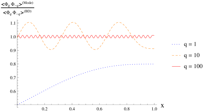
Fig. 1 shows ΦqΦq(Mode)ΦqΦq(BD)superscriptdelimited-⟨⟩subscriptΦ𝑞subscriptΦ𝑞𝑀𝑜𝑑𝑒superscriptdelimited-⟨⟩subscriptΦ𝑞subscriptΦ𝑞𝐵𝐷\frac{\left\langle\Phi_{\vec{q}}\Phi_{-\vec{q}}\right\rangle^{(Mode)}}{\left\langle\Phi_{\vec{q}}\Phi_{-\vec{q}}\right\rangle^{(BD)}} for q=1,10𝑞110q=1,10, and 100. For q=1𝑞1q=1, corresponding to a mode that is crossing the horizon at η=η0𝜂subscript𝜂0\eta=\eta_{0}, the ratio seems to settle well below unity, increasing monotonically until it plateaus for larger x𝑥x values, meaning that no equilibrium between ΦqΦq(Mode)superscriptdelimited-⟨⟩subscriptΦ𝑞subscriptΦ𝑞𝑀𝑜𝑑𝑒\left\langle\Phi_{\vec{q}}\Phi_{-\vec{q}}\right\rangle^{(Mode)} and ΦqΦq(BD)superscriptdelimited-⟨⟩subscriptΦ𝑞subscriptΦ𝑞𝐵𝐷\left\langle\Phi_{\vec{q}}\Phi_{-\vec{q}}\right\rangle^{(BD)} is reached. This is not surprising. Indeed, since all modes for which q[0,1]𝑞01q\in[0,1] are essentially frozen we should not expect anything dynamical to happen to their matching correlation functions. Thus it seems clear that for modes crossing the horizon or outside of it, information about the initial state is never lost.

As q𝑞q increases to 10 or even 100, ΦqΦq(Mode)ΦqΦq(BD)superscriptdelimited-⟨⟩subscriptΦ𝑞subscriptΦ𝑞𝑀𝑜𝑑𝑒superscriptdelimited-⟨⟩subscriptΦ𝑞subscriptΦ𝑞𝐵𝐷\frac{\left\langle\Phi_{\vec{q}}\Phi_{-\vec{q}}\right\rangle^{(Mode)}}{\left\langle\Phi_{\vec{q}}\Phi_{-\vec{q}}\right\rangle^{(BD)}} is characterized by an undamped oscillatory behavior about 111 with higher q𝑞q’s having smaller amplitudes. The absence of damping is due to the fact that taking a ratio of ΦqΦqdelimited-⟨⟩subscriptΦ𝑞subscriptΦ𝑞\left\langle\Phi_{\vec{q}}\Phi_{-\vec{q}}\right\rangle in different states erases the contributions of the scale factors, as can be seen from Eq. (II.3), hence the red-shifting of the modes due to the expansion of the universe is removed. Additionally, since our state can be viewed as a Bogoliubov transform of the BD state, |ϕq(x)|2superscriptsubscriptitalic-ϕ𝑞𝑥2|\phi_{q}(x)|^{2} just oscillates about |𝒰q(x)|2superscriptsubscript𝒰𝑞𝑥2|{\cal U}_{q}(x)|^{2} with constant amplitude. Given the form of ΦqΦqdelimited-⟨⟩subscriptΦ𝑞subscriptΦ𝑞\left\langle\Phi_{\vec{q}}\Phi_{-\vec{q}}\right\rangle the same should occur between ΦqΦq(Mode)superscriptdelimited-⟨⟩subscriptΦ𝑞subscriptΦ𝑞𝑀𝑜𝑑𝑒\left\langle\Phi_{\vec{q}}\Phi_{-\vec{q}}\right\rangle^{(Mode)} and ΦqΦq(BD)superscriptdelimited-⟨⟩subscriptΦ𝑞subscriptΦ𝑞𝐵𝐷\left\langle\Phi_{\vec{q}}\Phi_{-\vec{q}}\right\rangle^{(BD)}.

Refer to caption
Figure 1: The ratioΦqΦq(Mode)ΦqΦq(BD)superscriptdelimited-⟨⟩subscriptΦ𝑞subscriptΦ𝑞𝑀𝑜𝑑𝑒superscriptdelimited-⟨⟩subscriptΦ𝑞subscriptΦ𝑞𝐵𝐷\frac{\left\langle\Phi_{\vec{q}}\Phi_{-\vec{q}}\right\rangle^{(Mode)}}{\left\langle\Phi_{\vec{q}}\Phi_{-\vec{q}}\right\rangle^{(BD)}} for q=1,10,𝑞110q=1,10, and 100100100. For q=1𝑞1q=1 (dotted line) the ratio clearly does not asymptote to 111, while for q=10𝑞10q=10 and q=100𝑞100q=100 (dashed and solid lines, respectively) it oscillates about 111 without any damping, but with amplitude decreasing with increasing q𝑞q values. Such fine-grained curves do not observe equilibration.

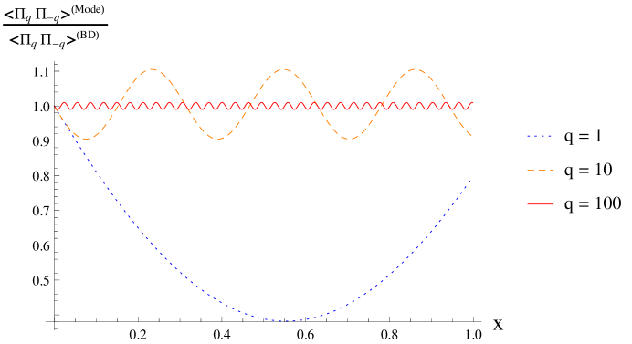
The ratio ΠqΠq(Mode)ΠqΠq(BD)superscriptdelimited-⟨⟩subscriptΠ𝑞subscriptΠ𝑞𝑀𝑜𝑑𝑒superscriptdelimited-⟨⟩subscriptΠ𝑞subscriptΠ𝑞𝐵𝐷\frac{\left\langle\Pi_{\vec{q}}\Pi_{-\vec{q}}\right\rangle^{(Mode)}}{\left\langle\Pi_{\vec{q}}\Pi_{-\vec{q}}\right\rangle^{(BD)}} in Fig. 2, presents similarities with Fig. 1 for q=10𝑞10q=10 and q=100𝑞100q=100, namely the ratio corresponding to such modes is oscillatory about an equilibrium value of 111 and undamped. Moreover for q=1𝑞1q=1, no approach to unity is observed.

Refer to caption
Figure 2: The ratio ΠqΠq(Mode)ΠqΠq(BD)superscriptdelimited-⟨⟩subscriptΠ𝑞subscriptΠ𝑞𝑀𝑜𝑑𝑒superscriptdelimited-⟨⟩subscriptΠ𝑞subscriptΠ𝑞𝐵𝐷\frac{\left\langle\Pi_{\vec{q}}\Pi_{-\vec{q}}\right\rangle^{(Mode)}}{\left\langle\Pi_{\vec{q}}\Pi_{-\vec{q}}\right\rangle^{(BD)}} for q=1,10𝑞110q=1,10, and 100. Similarly to what was observed in Fig. 1, it appears the ratio evaluated at q=1𝑞1q=1 does not approach 111, while ΠqΠq(Mode)ΠqΠq(BD)superscriptdelimited-⟨⟩subscriptΠ𝑞subscriptΠ𝑞𝑀𝑜𝑑𝑒superscriptdelimited-⟨⟩subscriptΠ𝑞subscriptΠ𝑞𝐵𝐷\frac{\left\langle\Pi_{\vec{q}}\Pi_{-\vec{q}}\right\rangle^{(Mode)}}{\left\langle\Pi_{\vec{q}}\Pi_{-\vec{q}}\right\rangle^{(BD)}} taken for q=10𝑞10q=10 or q=100𝑞100q=100 oscillates without damping about 111, with an amplitude that decreases as q𝑞q becomes higher. As in Fig. 1 no signs of equilibration are found.

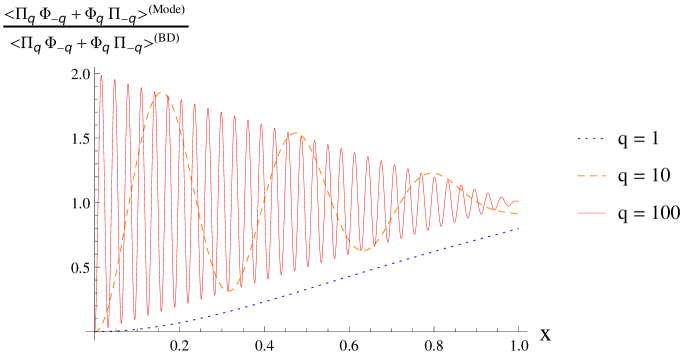
The last ratio of correlators, ΦqΠq+ΠqΦq(Mode)ΦqΠq+ΠqΦq(BD)superscriptdelimited-⟨⟩subscriptΦ𝑞subscriptΠ𝑞subscriptΠ𝑞subscriptΦ𝑞𝑀𝑜𝑑𝑒superscriptdelimited-⟨⟩subscriptΦ𝑞subscriptΠ𝑞subscriptΠ𝑞subscriptΦ𝑞𝐵𝐷\frac{\left\langle\Phi_{\vec{q}}\Pi_{-\vec{q}}+\Pi_{\vec{q}}\Phi_{-\vec{q}}\right\rangle^{(Mode)}}{\left\langle\Phi_{\vec{q}}\Pi_{-\vec{q}}+\Pi_{\vec{q}}\Phi_{-\vec{q}}\right\rangle^{(BD)}}, is shown in Fig. 3. When q=1𝑞1q=1, this quantity appears to grow monotonically for all x𝑥x, corroborating the absence of equilibrium for such corresponding modes. The striking feature of Fig. 3, manifesting itself when compared to Fig. 1 and 2, is that the ratios tend to oscillate about 111 for q>1𝑞1q>1, but now with an amplitude that diminishes as a function of time. The size of the oscillations is now damped linearly, while being constant in the first two plots. Such a disparity is due to the presence of scale factors in (II.3) that do not cancel upon taking a quotient of two-point functions evaluated in different states.
Refer to caption
Figure 3: The ratio ΠqΦq+ΦqΠq(Mode)ΠqΦq+ΦqΠq(BD)superscriptdelimited-⟨⟩subscriptΠ𝑞subscriptΦ𝑞subscriptΦ𝑞subscriptΠ𝑞𝑀𝑜𝑑𝑒superscriptdelimited-⟨⟩subscriptΠ𝑞subscriptΦ𝑞subscriptΦ𝑞subscriptΠ𝑞𝐵𝐷\frac{\left\langle\Pi_{\vec{q}}\Phi_{-\vec{q}}+\Phi_{\vec{q}}\Pi_{-\vec{q}}\right\rangle^{(Mode)}}{\left\langle\Pi_{\vec{q}}\Phi_{-\vec{q}}+\Phi_{\vec{q}}\Pi_{-\vec{q}}\right\rangle^{(BD)}} for q=1,10𝑞110q=1,10, and 100100100. Similar conclusions to the ones in Fig. 1 and 2 can be made, namely, the higher the q𝑞q-mode the smaller the amplitude of oscillations. However, contrary to the previous two figures, the ratios corresponding to q=10𝑞10q=10 and 100100100 oscillate about 111 with amplitude decreasing linearly.

Despite the described differences found when comparing Fig. 1, 2, and 3, we argue that one can draw similar conclusions regarding the lack of equilibration. It is not surprising that correlation functions for modes crossing, near crossing, or outside the horizon do not exhibit equilibration, as such modes freeze out. Moreover the oscillatory behavior shown for higher q𝑞q modes in Fig. 1 and 2 also does not reflect equilibration. At first glance, the curves in Fig. 3 seem to indicate an approach to the BD mode, since all curves approach unity over time. However, x1𝑥1x\rightarrow 1 corresponds to t+𝑡t\rightarrow+\infty for cosmic time t𝑡t. We feel the slowness of the approach to unity of the curves in Fig. 3 leaves us unconvinced that this quantity should be regarded as equilibrating. The q=1𝑞1q=1 and q=10𝑞10q=10 curves clearly do not actually reach unity as x1𝑥1x\rightarrow 1, and the same is true of the q=100𝑞100q=100 curve, although this is harder to see from the plot.

The lack of equilibration of the two-point functions for single modes is hardly the final word. After all one cannot learn about the equilibration of a box of gas by following a single energy eigenstate of the microscopic system, no matter how strongly the equilibration is realized overall. We next consider correlation functions averaged over a range of q𝑞q’s, as a way to represent coarse-graining. Although our setup is rather formal, we believe these averaged quantities bring us closer to representing realistic observables.

III.2.2 Quantities averaged over modes

We integrated all our two-point functions over finite ranges of q𝑞q: [1,3]13[1,3], [3,9]39[3,9], and [10,20]1020[10,20]. Such domains in q𝑞q have been chosen to demonstrate the difference between modes that sit inside the horizon (with large wavelengths for q[3,9]𝑞39q\in[3,9] or q𝑞q an order of magnitude away from horizon-crossing for q[10,30]𝑞1030q\in[10,30]) and those that are traversing or near the horizon. We have found that the general behaviors can be identified without including even higher values of q𝑞q. Our ratios then become ΦqΦq[qmin,qmax](Mode)ΦqΦq[qmin,qmax](BD)subscriptsuperscriptdelimited-⟨⟩subscriptΦ𝑞subscriptΦ𝑞𝑀𝑜𝑑𝑒subscript𝑞𝑚𝑖𝑛subscript𝑞𝑚𝑎𝑥subscriptsuperscriptdelimited-⟨⟩subscriptΦ𝑞subscriptΦ𝑞𝐵𝐷subscript𝑞𝑚𝑖𝑛subscript𝑞𝑚𝑎𝑥\frac{\left\langle\Phi_{\vec{q}}\Phi_{-\vec{q}}\right\rangle^{(Mode)}_{[q_{min},q_{max}]}}{\left\langle\Phi_{\vec{q}}\Phi_{-\vec{q}}\right\rangle^{(BD)}_{[q_{min},q_{max}]}}, ΠqΠq[qmin,qmax](Mode)ΠqΠq[qmin,qmax](BD)subscriptsuperscriptdelimited-⟨⟩subscriptΠ𝑞subscriptΠ𝑞𝑀𝑜𝑑𝑒subscript𝑞𝑚𝑖𝑛subscript𝑞𝑚𝑎𝑥subscriptsuperscriptdelimited-⟨⟩subscriptΠ𝑞subscriptΠ𝑞𝐵𝐷subscript𝑞𝑚𝑖𝑛subscript𝑞𝑚𝑎𝑥\frac{\left\langle\Pi_{\vec{q}}\Pi_{-\vec{q}}\right\rangle^{(Mode)}_{[q_{min},q_{max}]}}{\left\langle\Pi_{\vec{q}}\Pi_{-\vec{q}}\right\rangle^{(BD)}_{[q_{min},q_{max}]}},and ΦqΠq+ΠqΦq[qmin,qmax](Mode)ΦqΠq+ΠqΦq[qmin,qmax](BD),subscriptsuperscriptdelimited-⟨⟩subscriptΦ𝑞subscriptΠ𝑞subscriptΠ𝑞subscriptΦ𝑞𝑀𝑜𝑑𝑒subscript𝑞𝑚𝑖𝑛subscript𝑞𝑚𝑎𝑥subscriptsuperscriptdelimited-⟨⟩subscriptΦ𝑞subscriptΠ𝑞subscriptΠ𝑞subscriptΦ𝑞𝐵𝐷subscript𝑞𝑚𝑖𝑛subscript𝑞𝑚𝑎𝑥\frac{\left\langle\Phi_{\vec{q}}\Pi_{-\vec{q}}+\Pi_{\vec{q}}\Phi_{-\vec{q}}\right\rangle^{(Mode)}_{[q_{min},q_{max}]}}{\left\langle\Phi_{\vec{q}}\Pi_{-\vec{q}}+\Pi_{\vec{q}}\Phi_{-\vec{q}}\right\rangle^{(BD)}_{[q_{min},q_{max}]}}, where qminsubscript𝑞𝑚𝑖𝑛q_{min} is our lower limit of integration and qmaxsubscript𝑞𝑚𝑎𝑥q_{max} our upper limit.

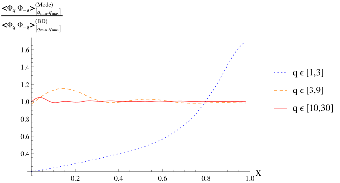
As shown in Fig. 4, integrating ΦqΦq[qmin,qmax](Mode)subscriptsuperscriptdelimited-⟨⟩subscriptΦ𝑞subscriptΦ𝑞𝑀𝑜𝑑𝑒subscript𝑞𝑚𝑖𝑛subscript𝑞𝑚𝑎𝑥\left\langle\Phi_{\vec{q}}\Phi_{-\vec{q}}\right\rangle^{(Mode)}_{[q_{min},q_{max}]} and ΦqΦq[qmin,qmax](BD)subscriptsuperscriptdelimited-⟨⟩subscriptΦ𝑞subscriptΦ𝑞𝐵𝐷subscript𝑞𝑚𝑖𝑛subscript𝑞𝑚𝑎𝑥\left\langle\Phi_{\vec{q}}\Phi_{-\vec{q}}\right\rangle^{(BD)}_{[q_{min},q_{max}]} over q𝑞q introduces damping in the ratio of the two for mode ranges well within the horizon, while averaging over the near-horizon-crossing range (q[1,3]𝑞13q\in[1,3]) does not. For the former modes, the ratios oscillate about 111 but a damping occurs over time such that the two-point functions eventually asymptote to 111. For q[10,30]𝑞1030q\in[10,30], the ratio clearly becomes 111, i.e, equilibration of ΦqΦq[qmin,qmax](Mode)subscriptsuperscriptdelimited-⟨⟩subscriptΦ𝑞subscriptΦ𝑞𝑀𝑜𝑑𝑒subscript𝑞𝑚𝑖𝑛subscript𝑞𝑚𝑎𝑥\left\langle\Phi_{\vec{q}}\Phi_{-\vec{q}}\right\rangle^{(Mode)}_{[q_{min},q_{max}]} with ΦqΦq[qmin,qmax](BD)subscriptsuperscriptdelimited-⟨⟩subscriptΦ𝑞subscriptΦ𝑞𝐵𝐷subscript𝑞𝑚𝑖𝑛subscript𝑞𝑚𝑎𝑥\left\langle\Phi_{\vec{q}}\Phi_{-\vec{q}}\right\rangle^{(BD)}_{[q_{min},q_{max}]} is reached. Looking at higher q𝑞q-modes, we observed that the higher the q𝑞q-domain the earlier the equilibration, since such modes have smaller amplitudes. Comparing with Fig. 1, we can infer that the damping is due to the integration over q𝑞q-modes. Hence we may conclude that, from the perspective of the field correlation functions, equilibrium is attained for sets of modes that start well inside the horizon, with q𝑞q of order 101010 and beyond.

Refer to caption
Figure 4: The ratio ΦqΦq[qmin,qmax](Mode)ΦqΦq[qmin,qmax](BD)subscriptsuperscriptdelimited-⟨⟩subscriptΦ𝑞subscriptΦ𝑞𝑀𝑜𝑑𝑒subscript𝑞𝑚𝑖𝑛subscript𝑞𝑚𝑎𝑥subscriptsuperscriptdelimited-⟨⟩subscriptΦ𝑞subscriptΦ𝑞𝐵𝐷subscript𝑞𝑚𝑖𝑛subscript𝑞𝑚𝑎𝑥\frac{\left\langle\Phi_{\vec{q}}\Phi_{-\vec{q}}\right\rangle^{(Mode)}_{[q_{min},q_{max}]}}{\left\langle\Phi_{\vec{q}}\Phi_{-\vec{q}}\right\rangle^{(BD)}_{[q_{min},q_{max}]}} integrated for q[1,3]𝑞13q\in[1,3], q[3,9]𝑞39q\in[3,9], and q[10,30]𝑞1030q\in[10,30]. For qmin=1subscript𝑞𝑚𝑖𝑛1q_{min}=1 and qmax=3subscript𝑞𝑚𝑎𝑥3q_{max}=3 (dotted line) the ratio clearly deviates from 111, corroborating the fact that modes near horizon-exit and beyond, do not equilibrate. For other domains [qmin,qmax]subscript𝑞𝑚𝑖𝑛subscript𝑞𝑚𝑎𝑥[q_{min},q_{max}] (dashed and solid lines) ΦqΦq[qmin,qmax](Mode)ΦqΦq[qmin,qmax](BD)subscriptsuperscriptdelimited-⟨⟩subscriptΦ𝑞subscriptΦ𝑞𝑀𝑜𝑑𝑒subscript𝑞𝑚𝑖𝑛subscript𝑞𝑚𝑎𝑥subscriptsuperscriptdelimited-⟨⟩subscriptΦ𝑞subscriptΦ𝑞𝐵𝐷subscript𝑞𝑚𝑖𝑛subscript𝑞𝑚𝑎𝑥\frac{\left\langle\Phi_{\vec{q}}\Phi_{-\vec{q}}\right\rangle^{(Mode)}_{[q_{min},q_{max}]}}{\left\langle\Phi_{\vec{q}}\Phi_{-\vec{q}}\right\rangle^{(BD)}_{[q_{min},q_{max}]}} oscillates about 111 with a clear damping over time.

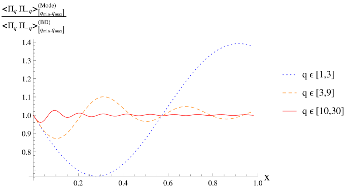
We may draw similar conclusions from Fig. 5 as in Fig. 4. For q[3,9]𝑞39q\in[3,9] and q[10,30]𝑞1030q\in[10,30], ΠqΠq[qmin,qmax](Mode)ΠqΠq[qmin,qmax](BD)subscriptsuperscriptdelimited-⟨⟩subscriptΠ𝑞subscriptΠ𝑞𝑀𝑜𝑑𝑒subscript𝑞𝑚𝑖𝑛subscript𝑞𝑚𝑎𝑥subscriptsuperscriptdelimited-⟨⟩subscriptΠ𝑞subscriptΠ𝑞𝐵𝐷subscript𝑞𝑚𝑖𝑛subscript𝑞𝑚𝑎𝑥\frac{\left\langle\Pi_{\vec{q}}\Pi_{-\vec{q}}\right\rangle^{(Mode)}_{[q_{min},q_{max}]}}{\left\langle\Pi_{\vec{q}}\Pi_{-\vec{q}}\right\rangle^{(BD)}_{[q_{min},q_{max}]}} appears oscillatory about the equilibrium position and damped. For the former domain, the ratio does not exactly achieve equilibrium but approaches it. It clearly hits 111 for q[10,30]𝑞1030q\in[10,30]. For qmin=1subscript𝑞𝑚𝑖𝑛1q_{min}=1, no equilibration occurs. Therefore, we may conclude that modes such that q𝑞q is of order 101010 and beyond equilibrate, from the point of view of the momentum correlator.
Refer to caption
Figure 5: The ratio ΠqΠq[qmin,qmax](Mode)ΠqΠq[qmin,qmax](BD)subscriptsuperscriptdelimited-⟨⟩subscriptΠ𝑞subscriptΠ𝑞𝑀𝑜𝑑𝑒subscript𝑞𝑚𝑖𝑛subscript𝑞𝑚𝑎𝑥subscriptsuperscriptdelimited-⟨⟩subscriptΠ𝑞subscriptΠ𝑞𝐵𝐷subscript𝑞𝑚𝑖𝑛subscript𝑞𝑚𝑎𝑥\frac{\left\langle\Pi_{\vec{q}}\Pi_{-\vec{q}}\right\rangle^{(Mode)}_{[q_{min},q_{max}]}}{\left\langle\Pi_{\vec{q}}\Pi_{-\vec{q}}\right\rangle^{(BD)}_{[q_{min},q_{max}]}} integrated for q[1,3]𝑞13q\in[1,3], q[3,9]𝑞39q\in[3,9], and q[10,30]𝑞1030q\in[10,30]. For qmin=1subscript𝑞𝑚𝑖𝑛1q_{min}=1 and qmax=3subscript𝑞𝑚𝑎𝑥3q_{max}=3 (dotted line) the ratio oscillates about 111 without damping, while for other ranges [qmin,qmax]subscript𝑞𝑚𝑖𝑛subscript𝑞𝑚𝑎𝑥[q_{min},q_{max}], the ratio damps out close to 111. For q[10,30]𝑞1030q\in[10,30] (solid line), it clearly achieves 111 for higher x𝑥x-values. In other words coarse-graining ΠqΠq[qmin,qmax](Mode)ΠqΠq[qmin,qmax](BD)subscriptsuperscriptdelimited-⟨⟩subscriptΠ𝑞subscriptΠ𝑞𝑀𝑜𝑑𝑒subscript𝑞𝑚𝑖𝑛subscript𝑞𝑚𝑎𝑥subscriptsuperscriptdelimited-⟨⟩subscriptΠ𝑞subscriptΠ𝑞𝐵𝐷subscript𝑞𝑚𝑖𝑛subscript𝑞𝑚𝑎𝑥\frac{\left\langle\Pi_{\vec{q}}\Pi_{-\vec{q}}\right\rangle^{(Mode)}_{[q_{min},q_{max}]}}{\left\langle\Pi_{\vec{q}}\Pi_{-\vec{q}}\right\rangle^{(BD)}_{[q_{min},q_{max}]}} over such modes results in equilibration of the numerator and denominator.

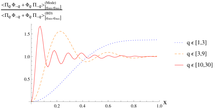
In Fig. 6, we observe a slight difference in the behavior of the lowest q𝑞q-range modes. For q[1,3]𝑞13q\in[1,3], ΦqΠq+ΠqΦq[qmin,qmax](Mode)ΦqΠq+ΠqΦq[qmin,qmax](BD)subscriptsuperscriptdelimited-⟨⟩subscriptΦ𝑞subscriptΠ𝑞subscriptΠ𝑞subscriptΦ𝑞𝑀𝑜𝑑𝑒subscript𝑞𝑚𝑖𝑛subscript𝑞𝑚𝑎𝑥subscriptsuperscriptdelimited-⟨⟩subscriptΦ𝑞subscriptΠ𝑞subscriptΠ𝑞subscriptΦ𝑞𝐵𝐷subscript𝑞𝑚𝑖𝑛subscript𝑞𝑚𝑎𝑥\frac{\left\langle\Phi_{\vec{q}}\Pi_{-\vec{q}}+\Pi_{\vec{q}}\Phi_{-\vec{q}}\right\rangle^{(Mode)}_{[q_{min},q_{max}]}}{\left\langle\Phi_{\vec{q}}\Pi_{-\vec{q}}+\Pi_{\vec{q}}\Phi_{-\vec{q}}\right\rangle^{(BD)}_{[q_{min},q_{max}]}} appears to plateau for x0.7𝑥0.7x\geq 0.7. Nevertheless no approach to unity can be found. This again proves that modes which are crossing or near-crossing the horizon do not equilibrate. Plots generated after integrating for q[3,9]𝑞39q\in[3,9], and q[10,30]𝑞1030q\in[10,30], show the same trends as in Fig. 4 and 5. Such modes approach (for qmin=3subscript𝑞𝑚𝑖𝑛3q_{min}=3) equilibrium or equilibrate (qmin=10subscript𝑞𝑚𝑖𝑛10q_{min}=10 and higher).

Refer to caption
Figure 6: The ratio ΦqΠq+ΠqΦq[qmin,qmax](Mode)ΦqΠq+ΠqΦq[qmin,qmax](BD)subscriptsuperscriptdelimited-⟨⟩subscriptΦ𝑞subscriptΠ𝑞subscriptΠ𝑞subscriptΦ𝑞𝑀𝑜𝑑𝑒subscript𝑞𝑚𝑖𝑛subscript𝑞𝑚𝑎𝑥subscriptsuperscriptdelimited-⟨⟩subscriptΦ𝑞subscriptΠ𝑞subscriptΠ𝑞subscriptΦ𝑞𝐵𝐷subscript𝑞𝑚𝑖𝑛subscript𝑞𝑚𝑎𝑥\frac{\left\langle\Phi_{\vec{q}}\Pi_{-\vec{q}}+\Pi_{\vec{q}}\Phi_{-\vec{q}}\right\rangle^{(Mode)}_{[q_{min},q_{max}]}}{\left\langle\Phi_{\vec{q}}\Pi_{-\vec{q}}+\Pi_{\vec{q}}\Phi_{-\vec{q}}\right\rangle^{(BD)}_{[q_{min},q_{max}]}} integrated for q[1,3]𝑞13q\in[1,3], q[3,9]𝑞39q\in[3,9], and q[10,30]𝑞1030q\in[10,30]. For the first domain of q𝑞q (dotted line), ΦqΠq+ΠqΦq[qmin,qmax](Mode)subscriptsuperscriptdelimited-⟨⟩subscriptΦ𝑞subscriptΠ𝑞subscriptΠ𝑞subscriptΦ𝑞𝑀𝑜𝑑𝑒subscript𝑞𝑚𝑖𝑛subscript𝑞𝑚𝑎𝑥\left\langle\Phi_{\vec{q}}\Pi_{-\vec{q}}+\Pi_{\vec{q}}\Phi_{-\vec{q}}\right\rangle^{(Mode)}_{[q_{min},q_{max}]} never equilibrates to ΦqΠq+ΠqΦq[qmin,qmax](BD)subscriptsuperscriptdelimited-⟨⟩subscriptΦ𝑞subscriptΠ𝑞subscriptΠ𝑞subscriptΦ𝑞𝐵𝐷subscript𝑞𝑚𝑖𝑛subscript𝑞𝑚𝑎𝑥\left\langle\Phi_{\vec{q}}\Pi_{-\vec{q}}+\Pi_{\vec{q}}\Phi_{-\vec{q}}\right\rangle^{(BD)}_{[q_{min},q_{max}]}. For qmin=3subscript𝑞𝑚𝑖𝑛3q_{min}=3 or 101010, the ratio is damped over time, and equilibrium is reached for q𝑞q-modes of order and greater than 101010.

In summary, when we ask whether the correlation functions of our state and the BD state approach one other, the answer seems to be that it depends on which modes are being considered. For those that remain well inside the horizon, we see the tendency of our state to approach the BD one, while for low q𝑞q-modes, this does not occur.

III.3 Stress-energy tensor

In terms of our variables x𝑥x and q𝑞q, Eq. (II.4) in the massless minimally coupled case becomes

T00=d3q(2π)3[(1x)62ΠqΠq+(1x)22q2ΦqΦq].delimited-⟨⟩subscriptsuperscript𝑇00superscript𝑑3𝑞superscript2𝜋3delimited-[]superscript1𝑥62delimited-⟨⟩subscriptΠ𝑞subscriptΠ𝑞superscript1𝑥22superscript𝑞2delimited-⟨⟩subscriptΦ𝑞subscriptΦ𝑞\left\langle T^{0}_{\phantom{b}0}\right\rangle=\int\frac{d^{3}q}{(2\pi)^{3}}\left[\frac{(1-x)^{6}}{2}\left\langle\Pi_{\vec{q}}\Pi_{-\vec{q}}\right\rangle+\frac{(1-x)^{2}}{2}q^{2}\left\langle\Phi_{\vec{q}}\Phi_{-\vec{q}}\right\rangle\right]. (28)

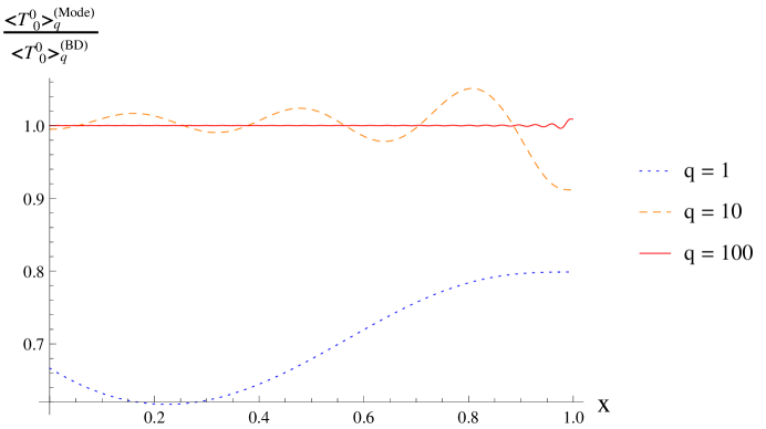
Let T00qsubscriptdelimited-⟨⟩subscriptsuperscript𝑇00𝑞\left\langle T^{0}_{\phantom{b}0}\right\rangle_{q} be the integrand of Eq. (28). Fig. 7 represents T00q(Mode)T00q(BD)superscriptsubscriptdelimited-⟨⟩subscriptsuperscript𝑇00𝑞𝑀𝑜𝑑𝑒superscriptsubscriptdelimited-⟨⟩subscriptsuperscript𝑇00𝑞𝐵𝐷\frac{\left\langle T^{0}_{\phantom{b}0}\right\rangle_{q}^{(Mode)}}{\left\langle T^{0}_{\phantom{b}0}\right\rangle_{q}^{(BD)}} for q=1,10𝑞110q=1,10 and 100. As seen when analyzing two-point functions, the ratio settles away from 111 when q=1𝑞1q=1 and exhibits an oscillatory behavior about 1 for the other q𝑞q-modes. However, contrary to our previous observations, the oscillations are characterized by an amplitude that increases as a function of x𝑥x. This is rather puzzling. Indeed, as discussed in section III.2, our state should be fully described by the two-point functions. T00qsubscriptdelimited-⟨⟩subscriptsuperscript𝑇00𝑞\left\langle T^{0}_{\phantom{b}0}\right\rangle_{q} itself is a function of two of them, in the massless and minimally coupled case. Thus we should expect to draw the same conclusions as in III.2. Note, however, that our conclusions about equilibration as perceived from the correlators originated after integrating them over q𝑞q. This suggests that we should adopt the same approach here.
Refer to caption
Figure 7: The ratio T00q(Mode)T00q(BD)superscriptsubscriptdelimited-⟨⟩subscriptsuperscript𝑇00𝑞𝑀𝑜𝑑𝑒superscriptsubscriptdelimited-⟨⟩subscriptsuperscript𝑇00𝑞𝐵𝐷\frac{\left\langle T^{0}_{\hskip 5.0pt0}\right\rangle_{q}^{(Mode)}}{\left\langle T^{0}_{\hskip 5.0pt0}\right\rangle_{q}^{(BD)}}for q=1𝑞1q=1, q=10𝑞10q=10 and q=100𝑞100q=100. For q=1𝑞1q=1, the ratio settles down well below the equilibrium position, while for q=10𝑞10q=10 and 100100100, it oscillates with increasing amplitude about 111. None of the curves present equilibration, similar to what was observed for other fine-grained quantities.
Refer to caption
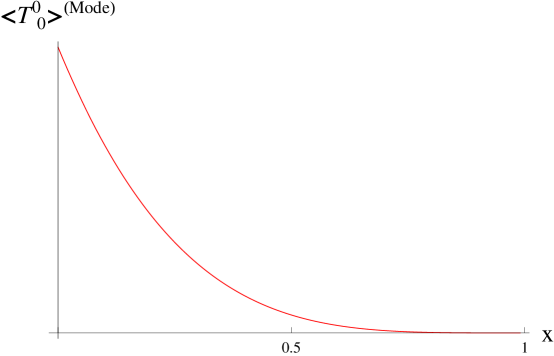
Figure 8: The stress-energy tensor T00[qmin,qmax](Mode)subscriptsuperscriptdelimited-⟨⟩subscriptsuperscript𝑇00𝑀𝑜𝑑𝑒subscript𝑞𝑚𝑖𝑛subscript𝑞𝑚𝑎𝑥\left\langle T^{0}_{\hskip 5.0pt0}\right\rangle^{(Mode)}_{[q_{min},q_{max}]} corresponding to T00q(Mode)superscriptsubscriptdelimited-⟨⟩subscriptsuperscript𝑇00𝑞𝑀𝑜𝑑𝑒\left\langle T^{0}_{\hskip 5.0pt0}\right\rangle_{q}^{(Mode)} integrated between q=1𝑞1q=1 and q=50𝑞50q=50. The expectation value monotonically approaches 00 as x𝑥x increases.

In Fig. 8 one can observe T00q(Mode)superscriptsubscriptdelimited-⟨⟩subscriptsuperscript𝑇00𝑞𝑀𝑜𝑑𝑒\left\langle T^{0}_{\phantom{b}0}\right\rangle_{q}^{(Mode)} integrated between q=1𝑞1q=1 and q=50𝑞50q=50. Let us label it T00[qmin,qmax](Mode)subscriptsuperscriptdelimited-⟨⟩subscriptsuperscript𝑇00𝑀𝑜𝑑𝑒subscript𝑞𝑚𝑖𝑛subscript𝑞𝑚𝑎𝑥\left\langle T^{0}_{\phantom{b}0}\right\rangle^{(Mode)}_{[q_{min},q_{max}]}. The distinctive feature of the plot is the fact that the integrated expectation value of the stress-energy tensor decreases monotonically as a function of x𝑥x, and eventually reaches 00. Given that ΦqΦqdelimited-⟨⟩subscriptΦ𝑞subscriptΦ𝑞\left\langle\Phi_{\vec{q}}\Phi_{-\vec{q}}\right\rangle falls off as a function of x𝑥x, and so does 1x1𝑥1-x (representing the scale factor in our rescaled equations) for x[0,1)𝑥01x\in[0,1), such a behavior makes sense from the point of view of those quantities. The correlator ΠqΠqdelimited-⟨⟩subscriptΠ𝑞subscriptΠ𝑞\left\langle\Pi_{\vec{q}}\Pi_{-\vec{q}}\right\rangle, however, rises as a function of x𝑥x. Since it does so as (1x)2superscript1𝑥2(1-x)^{-2}, the presence of (1x)6superscript1𝑥6(1-x)^{6} in front of ΠqΠqdelimited-⟨⟩subscriptΠ𝑞subscriptΠ𝑞\left\langle\Pi_{\vec{q}}\Pi_{-\vec{q}}\right\rangle in Eq. (28) is responsible for an overall decrease. In other words, the expansion of the universe takes care of any diverging behavior in ΠqΠqdelimited-⟨⟩subscriptΠ𝑞subscriptΠ𝑞\left\langle\Pi_{\vec{q}}\Pi_{-\vec{q}}\right\rangle. Looking at T00qsubscriptdelimited-⟨⟩subscriptsuperscript𝑇00𝑞\left\langle T^{0}_{\phantom{b}0}\right\rangle_{q} q𝑞q-mode per q𝑞q-mode the same declining trend was found, regardless of the chosen vacuum state. Equilibrium however was so far considered from the point of view of ratios of functions evaluated in our state to those evaluated in the Bunch-Davies state.
Refer to caption
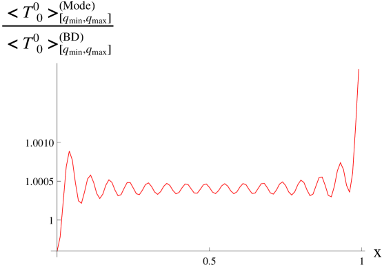
Figure 9: The ratio T00[qmin,qmax](Mode)T00[qmin,qmax](BD)subscriptsuperscriptdelimited-⟨⟩subscriptsuperscript𝑇00𝑀𝑜𝑑𝑒subscript𝑞𝑚𝑖𝑛subscript𝑞𝑚𝑎𝑥subscriptsuperscriptdelimited-⟨⟩subscriptsuperscript𝑇00𝐵𝐷subscript𝑞𝑚𝑖𝑛subscript𝑞𝑚𝑎𝑥\frac{\left\langle T^{0}_{\hskip 5.0pt0}\right\rangle^{(Mode)}_{[q_{min},q_{max}]}}{\left\langle T^{0}_{\hskip 5.0pt0}\right\rangle^{(BD)}_{[q_{min},q_{max}]}} obtained using qmin=1subscript𝑞𝑚𝑖𝑛1q_{min}=1 and qmax=50subscript𝑞𝑚𝑎𝑥50q_{max}=50 as our limits of integration. The ratio seems to oscillate about 1.00041.00041.0004 with an amplitude that decreases up to x=0.5𝑥0.5x=0.5 but keeps increasing afterward.

The quantity T00[qmin,qmax](Mode)T00[qmin,qmax](BD)subscriptsuperscriptdelimited-⟨⟩subscriptsuperscript𝑇00𝑀𝑜𝑑𝑒subscript𝑞𝑚𝑖𝑛subscript𝑞𝑚𝑎𝑥subscriptsuperscriptdelimited-⟨⟩subscriptsuperscript𝑇00𝐵𝐷subscript𝑞𝑚𝑖𝑛subscript𝑞𝑚𝑎𝑥\frac{\left\langle T^{0}_{\phantom{b}0}\right\rangle^{(Mode)}_{[q_{min},q_{max}]}}{\left\langle T^{0}_{\phantom{b}0}\right\rangle^{(BD)}_{[q_{min},q_{max}]}} is plotted in Fig. 9. Again, the limits of integration were chosen to be qmin=1subscript𝑞𝑚𝑖𝑛1q_{min}=1 and qmax=50subscript𝑞𝑚𝑎𝑥50q_{max}=50. The ratio appears to oscillate with damping until about x=0.5𝑥0.5x=0.5, but the amplitude of oscillations keeps increasing afterwards until very late times. This is quite unexpected as, from the point of view of the two-point functions, the ratios appeared damped monotonically with increasing x𝑥x values, after coarse-graining.

One could now ask why we used such low limits of integration. Using higher limits resulted in jaggedness in the plots coming from the higher frequency modes in the integral, which are difficult to integrate numerically. Since we are dealing with Hankel functions, themselves highly oscillatory, it is not astonishing that numerical integrators will have difficulty handling them. The fact that a lower step size in x𝑥x modified the observed jaggedness backs this hypothesis up.

Smaller steps in x𝑥x however means greater computing time. Analyzing plots with qmax>50subscript𝑞𝑚𝑎𝑥50q_{max}>50 revealed that the equilibrium position of oscillations in T00[qmin,qmax](Mode)T00[qmin,qmax](BD)subscriptsuperscriptdelimited-⟨⟩subscriptsuperscript𝑇00𝑀𝑜𝑑𝑒subscript𝑞𝑚𝑖𝑛subscript𝑞𝑚𝑎𝑥subscriptsuperscriptdelimited-⟨⟩subscriptsuperscript𝑇00𝐵𝐷subscript𝑞𝑚𝑖𝑛subscript𝑞𝑚𝑎𝑥\frac{\left\langle T^{0}_{\phantom{b}0}\right\rangle^{(Mode)}_{[q_{min},q_{max}]}}{\left\langle T^{0}_{\phantom{b}0}\right\rangle^{(BD)}_{[q_{min},q_{max}]}} would decrease to become closer to 111. Given the problems encountered after integrating numerically, we chose to call upon Riemann sums of T00qsubscriptdelimited-⟨⟩subscriptsuperscript𝑇00𝑞\left\langle T^{0}_{\phantom{b}0}\right\rangle_{q} instead of integrals. A step size in q𝑞q of order unity seemed appropriate and sufficient to draw our conclusions.

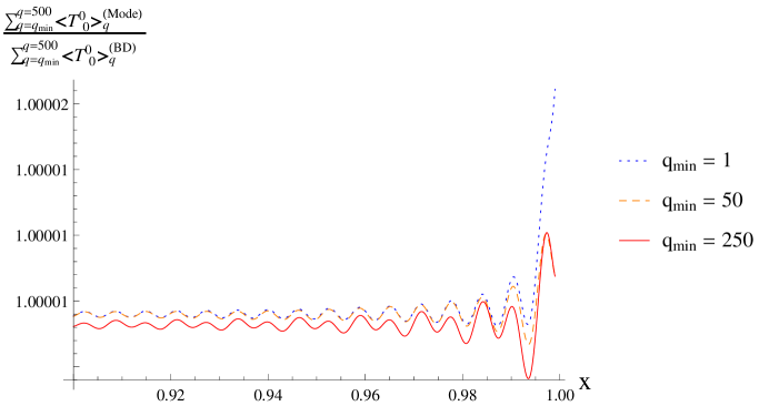
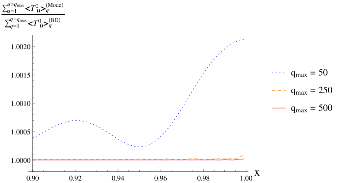
Fig. 10 shows q=1qmaxT00q(Mode)q=1qmaxT00q(BD)superscriptsubscript𝑞1subscript𝑞𝑚𝑎𝑥superscriptsubscriptdelimited-⟨⟩subscriptsuperscript𝑇00𝑞𝑀𝑜𝑑𝑒superscriptsubscript𝑞1subscript𝑞𝑚𝑎𝑥superscriptsubscriptdelimited-⟨⟩subscriptsuperscript𝑇00𝑞𝐵𝐷\frac{\sum\limits_{q=1}^{q_{max}}\left\langle T^{0}_{\phantom{b}0}\right\rangle_{q}^{(Mode)}}{\sum\limits_{q=1}^{q_{max}}\left\langle T^{0}_{\phantom{b}0}\right\rangle_{q}^{(BD)}} for qmax=50,subscript𝑞𝑚𝑎𝑥50q_{max}=50, 250, and 500 focusing on late times (x[0.900,0.999]𝑥0.9000.999x\in[0.900,0.999]). From the plots one can infer that the higher the qmaxsubscript𝑞𝑚𝑎𝑥q_{max} the lower the amplitude of oscillations of our ratio. Additionally, the equilibrium position of the latter gets arbitrarily near 1 as qmaxsubscript𝑞𝑚𝑎𝑥q_{max} increases. For a value qmax=500subscript𝑞𝑚𝑎𝑥500q_{max}=500, the ratio appears to remain at 1, up to 5 digits. This corroborates the fact that some equilibration process occurs as long as q𝑞q-modes of order 100 and more are included. One last important characteristic that can be found in the figure, is the fact that the quotient does not seem to diverge at very late times but flattens out.
Refer to caption
Figure 10: The quantity q=1qmaxT00q(Mode)q=1qmaxT00q(BD)superscriptsubscript𝑞1subscript𝑞𝑚𝑎𝑥superscriptsubscriptdelimited-⟨⟩subscriptsuperscript𝑇00𝑞𝑀𝑜𝑑𝑒superscriptsubscript𝑞1subscript𝑞𝑚𝑎𝑥superscriptsubscriptdelimited-⟨⟩subscriptsuperscript𝑇00𝑞𝐵𝐷\frac{\sum\limits_{q=1}^{q_{max}}\left\langle T^{0}_{\hskip 5.0pt0}\right\rangle_{q}^{(Mode)}}{\sum\limits_{q=1}^{q_{max}}\left\langle T^{0}_{\hskip 5.0pt0}\right\rangle_{q}^{(BD)}} for qmax=50subscript𝑞𝑚𝑎𝑥50q_{max}=50, 250, and 500, for x[0.900,0.999]𝑥0.9000.999x\in[0.900,0.999]. Higher qmaxsubscript𝑞𝑚𝑎𝑥q_{max} values correspond to lower amplitude of oscillations of the quotient, and an equilibrium position closer to 1. For qmax=500subscript𝑞𝑚𝑎𝑥500q_{max}=500, the ratio is indistinguishable from 1 up to four decimal places.

Another path to consider is changing our lower limit qminsubscript𝑞𝑚𝑖𝑛q_{min} in the integration, qmin=1subscript𝑞𝑚𝑖𝑛1q_{min}=1 corresponding to modes exiting the horizon. As seen in III.2 correlators characterizing such modes behave much differently than those for higher q𝑞q values. Fig. 11 shows q=qmin500T00q(Mode)q=qmin500T00q(BD)superscriptsubscript𝑞subscript𝑞𝑚𝑖𝑛500superscriptsubscriptdelimited-⟨⟩subscriptsuperscript𝑇00𝑞𝑀𝑜𝑑𝑒superscriptsubscript𝑞subscript𝑞𝑚𝑖𝑛500superscriptsubscriptdelimited-⟨⟩subscriptsuperscript𝑇00𝑞𝐵𝐷\frac{\sum\limits_{q=q_{min}}^{500}\left\langle T^{0}_{\phantom{b}0}\right\rangle_{q}^{(Mode)}}{\sum\limits_{q=q_{min}}^{500}\left\langle T^{0}_{\phantom{b}0}\right\rangle_{q}^{(BD)}} for qmin=1subscript𝑞𝑚𝑖𝑛1q_{min}=1, 50, and 250. Similar conclusions as the ones obtained in Fig. 10 can be drawn (except from the perspective of qminsubscript𝑞𝑚𝑖𝑛q_{min}), namely the higher the value of qminsubscript𝑞𝑚𝑖𝑛q_{min}, the closer the central value about which oscillations occur is to unity. Also, the amplitude decreases with higher qminsubscript𝑞𝑚𝑖𝑛q_{min}’s.

Refer to caption
Figure 11: The ratio q=qmin500T00q(Mode)q=qmin500T00q(BD)superscriptsubscript𝑞subscript𝑞𝑚𝑖𝑛500superscriptsubscriptdelimited-⟨⟩subscriptsuperscript𝑇00𝑞𝑀𝑜𝑑𝑒superscriptsubscript𝑞subscript𝑞𝑚𝑖𝑛500superscriptsubscriptdelimited-⟨⟩subscriptsuperscript𝑇00𝑞𝐵𝐷\frac{\sum\limits_{q=q_{min}}^{500}\left\langle T^{0}_{\hskip 5.0pt0}\right\rangle_{q}^{(Mode)}}{\sum\limits_{q=q_{min}}^{500}\left\langle T^{0}_{\hskip 5.0pt0}\right\rangle_{q}^{(BD)}} for qmin=1subscript𝑞𝑚𝑖𝑛1q_{min}=1, 50, and 250, for x[0.900,0.999]𝑥0.9000.999x\in[0.900,0.999]. The equilibrium position of the quotients and their amplitude of oscillations go down as qminsubscript𝑞𝑚𝑖𝑛q_{min} rises.

The stress-energy tensor seemed at first to be telling us a slightly different story about the equilibration of our state. However, focusing on the late time behavior of T00[qmin,qmax](Mode)T00[qmin,qmax](BD)subscriptsuperscriptdelimited-⟨⟩subscriptsuperscript𝑇00𝑀𝑜𝑑𝑒subscript𝑞𝑚𝑖𝑛subscript𝑞𝑚𝑎𝑥subscriptsuperscriptdelimited-⟨⟩subscriptsuperscript𝑇00𝐵𝐷subscript𝑞𝑚𝑖𝑛subscript𝑞𝑚𝑎𝑥\frac{\left\langle T^{0}_{\phantom{b}0}\right\rangle^{(Mode)}_{[q_{min},q_{max}]}}{\left\langle T^{0}_{\phantom{b}0}\right\rangle^{(BD)}_{[q_{min},q_{max}]}}, and/or changing the domain of q𝑞q-values to sum over, allows us to reconcile the conclusions coming from our different quantities. Indeed, lower q𝑞q-modes (of order unity) cross the horizon at earlier values of x𝑥x and have a much larger amplitude of oscillations as compared to the modes with q𝑞q-values that are one or more orders of magnitude higher.

Our relatively low values of qmaxsubscript𝑞𝑚𝑎𝑥q_{max} means any disparity from equilibrium would become mostly washed out by increasing qmaxsubscript𝑞𝑚𝑎𝑥q_{max} by a factor of 10 and using proper integration techniques. Nevertheless one should still expect the late time increase to be observed with increasing precision, even though it would decrease in amplitude. A reasonable explanation lies in the horizon-exit of the modes at different times. Such modes are still accounted for in our sums at late times, responsible for the seemingly anomalous rise of T00[qmin,qmax](Mode)T00[qmin,qmax](BD)subscriptsuperscriptdelimited-⟨⟩subscriptsuperscript𝑇00𝑀𝑜𝑑𝑒subscript𝑞𝑚𝑖𝑛subscript𝑞𝑚𝑎𝑥subscriptsuperscriptdelimited-⟨⟩subscriptsuperscript𝑇00𝐵𝐷subscript𝑞𝑚𝑖𝑛subscript𝑞𝑚𝑎𝑥\frac{\left\langle T^{0}_{\phantom{b}0}\right\rangle^{(Mode)}_{[q_{min},q_{max}]}}{\left\langle T^{0}_{\phantom{b}0}\right\rangle^{(BD)}_{[q_{min},q_{max}]}}. Hence, the effects observed in Fig. 9 should be attributed to the limit in precision, the bounds in q𝑞q of our numerical calculation, and horizon-crossing effects.

IV Conclusions

To check for the approach to equilibrium for any given system, said system has to be disturbed from the putative equilibrium state. Then, its relaxation, or lack thereof back to the original state can be studied. This is what we did here: we disturbed de Sitter space by attaching to it a flat space segment for conformal times ηη0𝜂subscript𝜂0\eta\leq\eta_{0}, and considered what happened to the quantum state of a test scalar field in this geometry. The claim being tested is that this state should relax to the “thermal” Bunch-Davies state.

The simplicity of the system allowed us to fully characterize the state by its various two-point functions and we used the ratios of these two-point functions in the disturbed state to their values in the BD state as our diagnostics of equilibration. We also used the stress-energy tensor as a check on whether our state evolved to the BD one.

What we found was that if we considered these quantities mode by mode there was no evidence of equilibration. Coarse-grained quantities (integrated over a range of q𝑞q-modes) did show evidence of equilibration in cases where the modes were well within the horizon. It seems that the importance of coarse-graining in our analysis here is no different than it is in more familiar equilibrating systems. Integrating our quantities over momentum modes that remained inside a horizon defined by η0subscript𝜂0\eta_{0}, we saw that they did equilibrate, and the smaller the wavelengths of our modes, the earlier the equilibration. Particular attention was given to the analysis of the momentum-energy tensor which, initially, presented disparities when compared to the other observables. The range of horizon-exit times of our modes, the necessity to restrict our domain in q𝑞q-space, and a finite precision in our numerical integrations accounted for such differences.

While our results corroborate the attractor behavior of the Bunch-Davies state, no notion of thermality was discussed. The Bunch-Davies state however is considered thermal Birrell and Davies (1982), upon calculation of how an Unruh-DeWitt detector responds when the field is placed in such a state. Such ambiguity will be investigated and hopefully alleviated in future work (Albrecht et al. (2014)) in which we address the thermality of our state, after developing a different way to calculate the response rate of an Unruh-DeWitt detector.

Acknowledgements.
We thank McCullen Sandora for useful discussions. R. H. was supported in part by the Department of Energy under grant DE-FG03-91-ER40682 as well as the John Templeton Foundation. He also thanks the Department of Physics at UC Davis for hospitality while this work was in progress. A. A. and B. R. were supported in part by DOE Grants DE-FG02-91ER40674 and DE-FG03- 91ER40674 and the National Science Foundation under Grant No. PHY11-25915.

References

  • Albrecht and Sorbo (2004) A. Albrecht and L. Sorbo, Phys. Rev. D 70, 063528 (2004), eprint arXiv:hep-th/0405270.
  • Albrecht (2009) A. Albrecht, J. Phys. Conf. Ser. 174, 012006 (2009), eprint arXiv:0906.1047 [gr-qc].
  • Birrell and Davies (1982) N. D. Birrell and P. C. W. Davies, Quantum Fields in curved space (Cambridge University Press, 1982).
  • Gibbons and Hawking (1977) G. W. Gibbons and S. W. Hawking, Phys. Rev. D 15, 2752 (1977).
  • Bunch and Davies (1978) T. Bunch and P. Davies, Proc. Roy. Soc. Lond. A 360, 117 (1978).
  • Schomblond and Spindel (1976) C. Schomblond and P. Spindel, Ann. Inst. Henri Poincaré Phys. Theor. 25, 67 (1976).
  • Bennett et al. (2012) C. L. Bennett et al., arXiv:astro-ph/1212.5225 (2012).
  • Ade et al (2013) P. A. R. Ade et al, arXiv:astro-ph/1303.5075 (2013).
  • Vilenkin and Ford (1982) A. Vilenkin and L. H. Ford, Phys. Rev. D 26, 1231 (1982).
  • Anderson et al. (2000) P. R. Anderson, W. Eaker, S. Habib, C. Molina-París, and E. Mottola, Phys. Rev. D 62, 124019 (2000), eprint arXiv:gr-qc/0005102.
  • Fischler et al. (2014a) W. Fischler, S. Kundu, and J. F. Pedraza, JHEP 0714, 021 (2014a), eprint arXiv:1311.5519 [hep-th].
  • Fischler et al. (2014b) W. Fischler, P. H. Nguyen, J. F. Pedraza, and W. Tangarife, JHEP 0814, 028 (2014b), eprint arXiv:1404.0347 [hep-th].
  • Singh et al. (2013a) S. Singh, C. Ganguly, and T. Padmanabhan, Phys. Rev. D 87, 104004 (2013a), eprint arXiv:1302.7177 [gr-qc].
  • Singh et al. (2013b) S. Singh, S. K. Modak, and T. Padmanabhan, Phys. Rev. D 88, 125020 (2013b), eprint arXiv:1308.4976 [gr-qc].
  • Boyanovsky et al. (1994) D. Boyanovsky, H. J. de Vega, and R. Holman, Phys. Rev. D 49, 2769 (1994), eprint arXiv:hep-ph/9310319.
  • Albrecht et al. (2014) A. Albrecht, B. J. Richard, and R. Holman, Work in progress (2014).