Leading order finite size effects with spins
for inspiralling compact binaries

Abstract

The leading order finite size effects due to spin, namely that of the cubic and quartic in spin interactions, are derived for the first time for generic compact binaries via the effective field theory for gravitating spinning objects. These corrections enter at the third and a half and fourth post-Newtonian orders, respectively, for rapidly rotating compact objects. Hence, we complete the leading order finite size effects with spin up to the fourth post-Newtonian accuracy. We arrive at this by augmenting the point particle effective action with new higher dimensional nonminimal coupling worldline operators, involving higher-order derivatives of the gravitational field, and introducing new Wilson coefficients, corresponding to constants, which describe the octupole and hexadecapole deformations of the object due to spin. These Wilson coefficients are fixed to unity in the black hole case. The nonminimal coupling worldline operators enter the action with the electric and magnetic components of the Weyl tensor of even and odd parity, coupled to even and odd worldline spin tensors, respectively. Moreover, the non relativistic gravitational field decomposition, which we employ, demonstrates a coupling hierarchy of the gravito-magnetic vector and the Newtonian scalar, to the odd and even in spin operators, respectively, which extends that of minimal coupling. This observation is useful for the construction of the Feynman diagrams, and provides an instructive analogy between the leading order spin-orbit and cubic in spin interactions, and between the leading order quadratic and quartic in spin interactions.

1 Introduction

Second-generation ground-based interferometers, such as Advanced LIGO LIGO , Advanced Virgo Virgo , and KAGRA Kagra , will start to operate in the next few years, making the anticipated direct detection of gravitational waves (GWs) a realistic prospect. Among the most promising sources in the accessible frequency band of such experiments are inspiralling binaries of compact objects, which can be treated analytically in terms of the post-Newtonian (PN) approximation of General Relativity Blanchet:2013haa . It turns out that even relative high order corrections beyond Newtonian gravity, such as the fourth PN (4PN) order, are crucial to obtain a successful detection from such sources, and furthermore to gain information about the inner structure of the constituents of the binary Yagi:2013baa . Moreover, such objects are expected to have large spins McClintock:2011zq , thus PN corrections involving spins should be completed to similar high orders as in the non spinning case, which was recently completed to 4PN order Damour:2014jta .

In particular, finite size effects involving spins should also be taken into account in order to obtain the required 4PN accuracy. The leading order (LO) finite size spin effects at the quadrupole level, i.e. of the LO spin-squared interaction, were first derived for black holes in D'Eath:1975vw ; Thorne:1984mz . Generic quadrupoles, required to describe neutron stars of different masses, were included already in Barker:1975ae , and the proportionality of the quadrupole to spin-squared was introduced in Poisson:1997ha . The LO spin-squared interaction enters already at the 2PN order for rapidly rotating generic compact objects. Yet, the next-to-leading order (NLO) spin-squared interaction at 3PN order was treated much later in the following series of works Porto:2008jj ; Steinhoff:2008ji ; Hergt:2008jn ; Hergt:2010pa . Finally, the LO cubic and quartic in spin interaction Hamiltonians for black hole binaries were computed in parts in Hergt:2007ha ; Hergt:2008jn . These corrections enter formally at the 2PN order, and for rapidly rotating compact objects at the 3.5PN and 4PN orders, respectively. However, these results were found to be incomplete in the test particle limit for the quartic in spin sector Steinhoff:2012rw .

In this work we derive for the first time the LO cubic and quartic in spin interaction potentials for generic compact binaries via the Effective Field Theory (EFT) for gravitating spinning objects Levi:2015msa . Hence, we complete the LO finite size effects with spin up to the 4PN accuracy. The novel self-contained EFT approach for the binary inspiral problem was introduced in Goldberger:2004jt ; Goldberger:2007hy , and an extension to spinning objects was first approached in Porto:2005ac . The EFT approach provides a systematic methodology to construct the action to arbitrary high accuracy in terms of local operators ordered by their relevance and their Wilson coefficients, which is invaluable for the obtainment of finite size effects. Moreover, the EFT approach also applies the efficient standard tools of Quantum Field Theory, such as Feynman diagrams. Indeed, we arrive at our results by augmenting the point particle action with new higher dimensional nonminimal coupling worldline operators, involving higher-order derivatives of the field, and introducing new Wilson coefficients, namely here spin-induced polarization coefficients, corresponding to constants, which describe the octupole and hexadecapole deformations of the object due to spin Levi:2015msa . These Wilson coefficients are fixed to unity in the black hole case. The nonminimal coupling worldline operators enter the action with the electric and magnetic components of the Weyl tensor of even and odd parity, coupled to even and odd worldline spin tensors, respectively.

Moreover, another advantageous practice in the EFT approach is the use of the non relativistic gravitational (NRG) fields, which were introduced in Kol:2007bc . The NRG decomposition of spacetime is essentially a reduction over the time dimension, and therefore it is the sensible decomposition for the PN limit Kol:2010ze . Indeed, the NRG field decomposition, which we employ, demonstrates a coupling hierarchy of the gravito-magnetic vector and the Newtonian scalar to the odd and even in spin operators, respectively, which extends that of minimal coupling, as was illustrated for the spin interactions in Levi:2008nh ; Levi:2010zu ; Levi:2011eq . This observation is very useful for the construction of the Feynman diagrams, and provides an instructive analogy between the LO spin-orbit and cubic in spin interactions, and between the LO quadratic and quartic in spin interactions.

The outline of the paper is as follows. In section 2 we review and present the new ingredients in the EFT formulation for finite size effects with spins to the order required in this work Levi:2015msa . In section 3 we derive the complete LO cubic in spin interaction potential for generic compact objects through the evaluation of the relevant Feynman diagrams, and we compare to the ADM Hamiltonian result for a black hole binary. In section 4 we similarly derive the complete LO quartic in spin interaction potential for generic compact objects, and we correct the corresponding ADM Hamiltonian result for the black hole binary case. Finally, in section 5 we summarize our main conclusions.

Throughout this paper we use $c\equiv 1$, $\eta_{\mu\nu}\equiv\text{Diag}[1,-1,-1,-1]$, and the convention for the Riemann tensor is $R^{\mu}{}_{\nu\alpha\beta}\equiv\partial_{\alpha}\Gamma^{\mu}_{\nu\beta}-\partial_{\beta}\Gamma^{\mu}_{\nu\alpha}+\Gamma^{\mu}_{\lambda\alpha}\Gamma^{\lambda}_{\nu\beta}-\Gamma^{\mu}_{\lambda\beta}\Gamma^{\lambda}_{\nu\alpha}$. Greek letters denote indices in the global coordinate frame. Spatial tensor indices are denoted with lowercase Latin letters from the middle of the alphabet, whereas uppercase ones denote particle labels. The scalar triple product appears here with no brackets, i.e. $\vec{a}\times\vec{b}\cdot\vec{c}\equiv(\vec{a}\times\vec{b})\cdot\vec{c}$.

2 Spin-induced finite size effects via the effective field theory for spin

In this section we present the effective action, that removes the scale of the compact objects in the EFT approach, and augment the point particle action, as required in order to take into account finite size effects with spins. For the construction of the spin-induced nonminimal couplings we follow the EFT for spin in Levi:2015msa , where an equivalent approach for generic tidal interactions is found in Bini:2012gu . For the Feynman rules we employ here the NRG fields Kol:2007bc ; Kol:2010ze , which continue to play a central role in the construction of the Feynman diagrams also in spin interactions, as will be seen in the next sections. Thus, their central role in spin interactions extends beyond the minimal coupling case, which was illustrated in Levi:2008nh ; Levi:2010zu ; Levi:2011eq .

We recall that the effective action, describing the binary system, is given by

$$S=S_{\text{g}}+\sum_{I=1}^{2}S_{\text{(I)pp}},$$ (1)

where $S_{\text{g}}$ is the pure gravitational action, and $S_{\text{(I)pp}}$ is the worldline point particle action for each of the two particles in the binary. The gravitational action is the usual Einstein-Hilbert action plus a gauge-fixing term, which we choose as the fully harmonic gauge, such that we have

$$S_{\text{g}}=S_{\text{EH}}+S_{\text{GF}}=-\frac{1}{16\pi G}\int d^{4}x\sqrt{g}\,R+\frac{1}{32\pi G}\int d^{4}x\sqrt{g}\,g_{\mu\nu}\Gamma^{\mu}\Gamma^{\nu},$$ (2)

where $\Gamma^{\mu}\equiv\Gamma^{\mu}_{\rho\sigma}g^{\rho\sigma}$.

In terms of the NRG fields $\phi$, $A_{i}$, $\gamma_{ij}\equiv\delta_{ij}+\sigma_{ij}$, the metric reads

$$g_{\mu\nu} =\left(\begin{array}[]{cc}e^{2\phi}&\quad-e^{2\phi}A_{j}\\ -e^{2\phi}A_{i}&\quad-e^{-2\phi}\gamma_{ij}+e^{2\phi}A_{i}A_{j}\end{array}\right) \simeq\left(\begin{array}[]{cc}1+2\phi&\quad-A_{j}\\ -A_{i}&\quad-\delta_{ij}+2\phi\delta_{ij}\end{array}\right),$$ (7)

where we have written the approximation in the weak field limit up to linear order in the fields as required in this work.

The NRG scalar and vector field propagators in the harmonic gauge are given by

$$\parbox{51.21495pt}{\includegraphics[scale={0.6}]{frg1.eps}}= \langle{~{}\phi(x_{1})}~{}~{}{\phi(x_{2})~{}}\rangle=~{}~{}~{}~{}4\pi G~{}~{}~{}\int\frac{d^{d}\vec{k}}{\left(2\pi\right)^{d}}\frac{e^{i\vec{k}\cdot\left(\vec{x}_{1}-\vec{x}_{2}\right)}}{k^{2}}~{}\delta(t_{1}-t_{2}),$$ (8)

$$\parbox{51.21495pt}{\includegraphics[scale={0.6}]{frg2.eps}}= \langle{A_{i}(x_{1})}~{}{A_{j}(x_{2})}\rangle=-16\pi G~{}\delta_{ij}\int\frac{d^{d}\vec{k}}{\left(2\pi\right)^{d}}\frac{e^{i\vec{k}\cdot\left(\vec{x}_{1}-\vec{x}_{2}\right)}}{k^{2}}~{}\delta(t_{1}-t_{2}).$$ (9)

Next, we recall that the minimal coupling part of the point particle action of each of the particles with spins Hanson:1974qy ; Bailey:1975fe ; Porto:2005ac ; Levi:2010zu is given by

$$S_{\text{pp}}= \int d\lambda\left[-m\sqrt{u^{2}}-\frac{1}{2}S_{\mu\nu}\Omega^{\mu\nu}\right],$$ (10)

where $\lambda$ is the affine parameter, $u^{\mu}\equiv dx^{\mu}/d\lambda$ is the 4-velocity, and $\Omega^{\mu\nu}$, $S_{\mu\nu}$ are the angular velocity and spin tensors of the particle, respectively Levi:2015msa . Considering this point particle action in eq. (1), the LO monopole-monopole interaction, namely the Newtonian interaction, which involves no spin, and the LO dipole-monopole interaction, namely the linear in spin LO spin-orbit interaction, are derived. These are obtained using the following Feynman rules we present, which are also those required to the order that we are considering in this work. Here we follow the same gauge choices and conventions as in Levi:2015msa , see section 5.3 there.

For the one-graviton couplings to the worldline mass, we have

$$\parbox{34.1433pt}{\includegraphics[scale={0.6}]{frm1.eps}}= -m\int dt~{}\phi,$$ (11)

$$\parbox{34.1433pt}{\includegraphics[scale={0.6}]{frm2.eps}}= ~{}m\int dt~{}A_{i}v^{i},$$ (12)

where the heavy solid lines represent the worldlines, and the spherical black blobs represent the masses on the worldline.

The Feynman rules for the one-graviton couplings to the worldline spin are:

$$\parbox{34.1433pt}{\includegraphics[scale={0.6}]{frs1.eps}}= \frac{1}{2}\int dt\,\,\left[\epsilon_{ijk}S_{k}\partial_{i}A_{j}\right],$$ (13)

$$\parbox{34.1433pt}{\includegraphics[scale={0.6}]{frs2.eps}}= 2\int dt\,\,\left[\epsilon_{ijk}S_{k}v^{i}\partial_{j}\phi\right],$$ (14)

where $\epsilon_{ijk}$ is the 3-dimensional Levi-Civita symbol, such that $S_{ij}=\epsilon_{ijk}S_{k}$, and the oval gray blobs represent the spins on the worldline. Note that the Feynman rules here contain only spatial components of the spin tensor, since the rotational gauge fixing is applied at the level of the point particle action, and thus the unphysical degrees of freedom of spin are already eliminated. Our rotational variables are ultimately fixed to the canonical gauge Levi:2015msa .

In order to take into account finite size effects with spins the point particle action should be extended beyond minimal coupling, see section 4 of Levi:2015msa for the complete treatment. Higher dimensional operators are introduced into the action, constructed with the Riemann tensor, which for a vacuum solution field is equivalent to the Weyl tensor, using its even and odd parity components. $E_{\mu\nu}$ is the electric component of the Weyl tensor, namely

$$E_{\mu\nu}\equiv R_{\mu\alpha\nu\beta}u^{\alpha}u^{\beta},$$ (15)

and $B_{\mu\nu}$ is the magnetic component of the Weyl tensor, that is

$$B_{\mu\nu}\equiv\frac{1}{2}\epsilon_{\alpha\beta\gamma\mu}R^{\alpha\beta}_{\quad\delta\nu}u^{\gamma}u^{\delta},$$ (16)

where $\epsilon_{\alpha\beta\gamma\mu}$ is the Levi-Civita tensor. The LO PN finite size effects are due to spin-induced multipoles, for which only linear in curvature operators should be considered.

These higher order operators are constructed according to the symmetries of the effective action Levi:2015msa . The crucial symmetries to consider for the construction of nonminimal couplings are parity invariance, and SO(3) invariance of the body-fixed triad, where we start with a timelike basis vector, satisfying $e_{[0]}{}^{\mu}=u^{\mu}/\sqrt{u^{2}}$, which amounts to a covariant gauge condition for the worldline tetrad. We also recall here that permanent multipole moments, beside mass and spin, are assumed to vanish, and that parity violation can be neglected for macroscopic compact objects in general relativity. The building blocks of these higher order operators are then spin-induced multipoles and curvature components with covariant derivatives, which are considered in the body-fixed frame, where they form irreducible representations of SO(3). Due to parity invariance the tensors, which contain the even-parity electric and odd-parity magnetic curvature components, should be contracted with an even and odd number of the spin vector, respectively, of an equal tensor rank, where the spin vector $S^{\mu}$ is defined here by

$$S^{\mu}\equiv\frac{1}{2}\epsilon_{\alpha\beta\gamma\mu}S^{\alpha\beta}\frac{u^{\gamma}}{\sqrt{u^{2}}}.$$ (17)

Finally, these nonminimal couplings carry Wilson coefficients, which encode the internal structure of the object.

For the LO spin-squared finite size effects the nonminimal coupling operator, which is added to the action Levi:2015msa , is given by

$$L_{\text{ES}^{2}}= -\frac{C_{\text{ES}^{2}}}{2m}\frac{E_{\mu\nu}}{\sqrt{u^{2}}}S^{\mu}S^{\nu}.$$ (18)

$C_{\text{ES}^{2}}$ is the Wilson coefficient Porto:2008jj , corresponding to the quadrupole deformation of the object due to spin, which was introduced in Poisson:1997ha , where the proportionality factor was called $a$. The spin-squared operator presented in eq. (18) is equivalent to that in Porto:2008jj , as the building blocks of the spin-induced nonminimal couplings, considered in the body-fixed frame, are traceless and orthogonal to the 4-velocity Levi:2015msa .

Considering this addition to the point particle action in eq. (10) and eq. (1), the LO quadrupole-monopole interaction, that is the LO spin-squared interaction, is derived, using the following Feynman rules we present, required to the order that we are considering in this work. The Feynman rules for the one-graviton couplings to the worldline spin-squared are given by

$$\parbox{34.1433pt}{\includegraphics[scale={0.6}]{frsqphi.eps}}= \int dt\,\,\left[\frac{C_{\text{ES}^{2}}}{2m}\left(S^{i}S^{j}\partial_{i}\partial_{j}\phi-S^{2}\partial_{i}\partial_{i}\phi\right)\right],$$ (19)

$$\parbox{34.1433pt}{\includegraphics[scale={0.6}]{frsqA.eps}}= \int dt\,\,\left[-\frac{C_{\text{ES}^{2}}}{2m}\left(S^{i}S^{j}\left(\partial_{i}\partial_{j}A_{l}v^{l}-\partial_{i}\partial_{l}A_{j}v^{l}-\partial_{i}\partial_{t}A_{j}\right)\right.\right.$$

$$\qquad\qquad\qquad\left.\left.-S^{2}\left(\partial_{i}\partial_{i}A_{k}v^{k}-\partial_{i}\partial_{k}A_{i}v^{k}-\partial_{i}\partial_{t}A_{i}\right)\right)\right],$$ (20)

where the square black boxes represent the $ES^{2}$ spin-squared operators on the worldlines. Note that in spite of naive power counting only the first terms in eqs. (19), (2), actually contribute here at LO. Using the leading coupling of the spin-squared to the Newtonian scalar in eq. (19), contracted with the corresponding leading mass coupling in eq. (11), we obtain the single Feynman diagram, which makes up the well-known LO spin-squared interaction Barker:1975ae ; Poisson:1997ha , shown in figure 1.

Figure 1: LO spin-squared interaction Feynman diagram. This diagram should be included together with its mirror image. This is a quadrupole-monopole interaction. Note the analogy with the Newtonian interaction.

The value of the Feynman diagram for the LO spin-squared interaction is given by

$$\text{Fig.~{}1}= \frac{1}{2}C_{1\text{(ES${}^{2}$)}}\frac{Gm_{2}}{m_{1}r^{3}}\left[S_{1}^{2}-3\left(\vec{S}_{1}\cdot\vec{n}\right)^{2}\right],$$ (21)

where $\vec{r}\equiv\vec{x}_{1}-\vec{x}_{2}$, $r\equiv\sqrt{{\vec{r}}^{2}}$, $\vec{n}\equiv\vec{r}/r$, and the LO spin-squared potential just equals $V_{\text{S${}_{1}^{2}$}}^{\text{LO}}=-\text{Fig.~{}1}$. Notice that this is a purely Newtonian effect, and that the worldline spin-squared acts just like a generic mass quadrupole.

In this work we want to complete the LO octupole and hexadecapole levels in the spins, since these contribute up to the 4PN accuracy for rapidly rotating compact objects. For that, the point particle action should be extended to LO cubic and quartic order in the spin Levi:2015msa .

The cubic in spin operator, that should be added here Levi:2015msa , is given by

$$L_{\text{BS}^{3}}= -\frac{C_{\text{BS}^{3}}}{6m^{2}}\frac{D_{\lambda}B_{\mu\nu}}{\sqrt{u^{2}}}S^{\mu}S^{\nu}S^{\lambda},$$ (22)

where $D_{\lambda}$ denotes the covariant derivative. We have introduced here $C_{\text{BS}^{3}}$, which is the Wilson coefficient, or constant describing the octupole deformation due to spin.

The Feynman rules for the one-graviton couplings to the worldline cubic spin are then given by

$$\parbox{34.1433pt}{\includegraphics[scale={0.6}]{frs3A.eps}}= \int dt\,\,\left[-\frac{C_{\text{BS}^{3}}}{12m^{2}}S^{i}S^{j}\epsilon_{klm}S^{m}\partial_{i}\partial_{j}\partial_{k}A_{l}\right],$$ (23)

$$\parbox{34.1433pt}{\includegraphics[scale={0.6}]{frs3phi.eps}}= \int dt\,\,\left[\frac{C_{\text{BS}^{3}}}{3m^{2}}S^{i}S^{j}\epsilon_{klm}S^{m}\partial_{i}\partial_{j}\partial_{k}\phi\,v^{l}\right],$$ (24)

where the rectangular gray boxes represent the $BS^{3}$ cubic spin operators on the worldlines. Here we have only included terms, which contribute at this order. Note that here it is the gravito-magnetic vector, which is the leading one in the hierarchy of coupling in the magnetic component of the Weyl tensor in the worldline cubic spin operator.

The quartic in spin operator, that should be added here Levi:2015msa , is given by

$$L_{\text{ES}^{4}}=\frac{C_{\text{ES}^{4}}}{24m^{3}}\frac{D_{\kappa}D_{\lambda}E_{\mu\nu}}{\sqrt{u^{2}}}S^{\mu}S^{\nu}S^{\lambda}S^{\kappa}.$$ (25)

We have introduced here $C_{\text{ES}^{4}}$, which is the Wilson coefficient, or constant describing the hexadecapole deformation due to spin.

Then, the Feynman rule for the one-graviton coupling to the worldline quartic spin is given by

$$\parbox{34.1433pt}{\includegraphics[scale={0.6}]{frs4phi.eps}}= \int dt\,\,\left[-\frac{C_{\text{ES}^{4}}}{24m^{3}}S^{i}S^{j}S^{k}S^{l}\partial_{i}\partial_{j}\partial_{k}\partial_{l}\phi\right],$$ (26)

where the crossed black box represents the $ES^{4}$ quartic spin operator on the worldline. Here again we have omitted terms, which actually only contribute beyond LO. Note that here it is again the Newtonian scalar, which is the leading one in the hierarchy of coupling in the electric component of the Weyl tensor in the worldline quartic spin operator.

3 Leading order cubic in spin interaction

The LO cubic and quartic in spin interaction Hamiltonians for the black hole binary case were approached in parts in Hergt:2007ha ; Hergt:2008jn . These corrections enter formally at the 2PN order, and at the 3.5PN and 4PN orders, respectively, for rapidly rotating compact objects. In this section and the next we derive these interaction potentials for any generic compact binary from the EFT for spin Levi:2015msa , where we construct these complete interactions in a direct and instructive manner.

3.1 Feynman diagrams

The cubic in spin interaction contains two kinds of interaction: a quadrupole-dipole interaction, and an octupole-monopole one. Each of these two interactions is analogous to the LO spin-orbit interaction, which is a dipole-monopole interaction. The correspondence is between even and odd parity multipole moments of the spin, such that the quadrupole and octupole moments correspond to the monopole (mass) and dipole (spin), respectively. We recall from figure 1 in section IV of Levi:2010zu , that the LO spin-orbit interaction contains two contributing Feynman diagrams, mediated by one-graviton exchanges of the gravito-magnetic vector and the Newtonian scalar of the NRG fields. Therefore, we expect to have here four contributing Feynman diagrams, two for each of the two kinds of interaction, that make up the cubic in spin interaction.

Indeed, the four contributing Feynman diagrams can be seen here in figure 2, where on the left diagrams (a) and (b), we have the quadrupole-dipole interaction, and on the right diagrams (c) and (d), we have the octupole-monopole interaction. These diagrams are obtained by the following contractions: in figure 2(a) the LO worldline spin coupling to the gravito-magnetic vector from eq. (13) is contracted with the corresponding quadrupole coupling in eq. (2); in figure 2(b) we contract the LO worldline spin quadrupole coupling to the Newtonian scalar from eq. (19) with the corresponding spin coupling in eq. (14); in figure 2(c) the LO worldline spin octupole coupling to the gravito-magnetic vector from eq. (23) is contracted with the corresponding mass coupling in eq. (12); finally, in figure 2(d) the LO worldline mass coupling to the Newtonian scalar from eq. (11) is contracted with the corresponding spin octupole coupling in eq. (24).

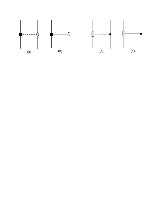
Figure 2: LO cubic in spin interaction Feynman diagrams. These diagrams should be included together with their mirror images. On the left pair we have the quadrupole-dipole interaction, and on the right pair we have the octupole-monopole one. Note the analogy of each pair with the LO spin-orbit interaction in figure 1 of Levi:2010zu .

Hence, the values of the Feynman diagrams of the LO cubic in spin interaction are given by the following:

$$\text{Fig.~{}2(a)}= -3\frac{C_{1\text{(ES${}^{2}$)}}G}{m_{1}r^{4}}\left[S_{1}^{2}\,\vec{S}_{2}\cdot\vec{n}\times\vec{v}_{1}+2\vec{S}_{1}\cdot\vec{n}\,\vec{S}_{2}\cdot\vec{S}_{1}\times\vec{v}_{1}-5\left(\vec{S}_{1}\cdot\vec{n}\right)^{2}\vec{S}_{2}\cdot\vec{n}\times\vec{v}_{1}\right]$$

$$-3\frac{C_{1\text{(ES${}^{2}$)}}G}{m_{1}r^{3}}\left[\dot{\vec{S}}_{1}\cdot\vec{n}\,\vec{n}\cdot\vec{S}_{1}\times\vec{S}_{2}+\vec{S}_{1}\cdot\vec{n}\,\vec{n}\cdot\dot{\vec{S}}_{1}\times\vec{S}_{2}\right],$$ (27)

$$\text{Fig.~{}2(b)}= \,3\frac{C_{1\text{(ES${}^{2}$)}}G}{m_{1}r^{4}}\left[S_{1}^{2}\,\vec{S}_{2}\cdot\vec{n}\times\vec{v}_{2}+2\vec{S}_{1}\cdot\vec{n}\,\vec{S}_{2}\cdot\vec{S}_{1}\times\vec{v}_{2}-5\left(\vec{S}_{1}\cdot\vec{n}\right)^{2}\vec{S}_{2}\cdot\vec{n}\times\vec{v}_{2}\right],$$ (28)

$$\text{Fig.~{}2(c)}= \,C_{1\text{(BS${}^{3}$)}}\frac{Gm_{2}}{m_{1}^{2}r^{4}}\vec{S}_{1}\cdot\vec{n}\times\vec{v}_{2}\left[S_{1}^{2}-5\left(\vec{S}_{1}\cdot\vec{n}\right)^{2}\right],$$ (29)

$$\text{Fig.~{}2(d)}= -C_{1\text{(BS${}^{3}$)}}\frac{Gm_{2}}{m_{1}^{2}r^{4}}\vec{S}_{1}\cdot\vec{n}\times\vec{v}_{1}\left[S_{1}^{2}-5\left(\vec{S}_{1}\cdot\vec{n}\right)^{2}\right].$$ (30)

The evaluation of the diagrams here is straightforward. Yet, note that the value of diagram 2(b) depends on the choice of the spin gauge. Following Levi:2015msa , after the covariant gauge is first inserted, and spin gauge freedom is incorporated in the action, an extra term from minimal coupling is added Levi:2015msa , and is expected to supplement the potential here.

3.2 Effective potential and Hamiltonian

As we noted in the end of the previous section, we recall that we have an addition from the extra minimal coupling term of Levi:2015msa , coming from the incorporation of spin gauge freedom in the rotational minimal coupling term, which enters already at the LO spin-orbit sector. This addition contributes here only the kinematic piece, similar to that noted in eq. (72) of Levi:2010zu , given by

$$L_{\text{SSS(extra)}}^{\text{LO}}=\frac{1}{2}\vec{S}_{1}\cdot\vec{v}_{1}\times\vec{a}_{1}+1\leftrightarrow 2,$$ (31)

and is acceleration dependent. We proceed then to eliminate the acceleration in this extra piece by making a redefinition of the position variables $\Delta\vec{x}_{I}$, as explained in Levi:2015msa , according to

$$\vec{x}_{1}\rightarrow\vec{x}_{1}+\frac{1}{2m_{1}}\vec{S}_{1}\times\vec{v}_{1},$$ (32)

and similarly for particle 2 with $1\leftrightarrow 2$. As explained in Damour:1990jh ; Levi:2014sba the linear shift in the position variables, corresponds to a substitution of the relevant EOM. Here these arise from the LO quadratic in spin sectors, and are given by

$$m_{1}\vec{a}_{1\text{(SS)}}= -\frac{3}{2}C_{1\text{(ES${}^{2}$)}}\frac{Gm_{2}}{m_{1}r^{4}}\left[\left(S_{1}^{2}-5\left(\vec{S}_{1}\cdot\vec{n}\right)^{2}\right)\vec{n}+2\vec{S}_{1}\cdot\vec{n}\vec{S}_{1}\right]+1\leftrightarrow 2$$

$$-\frac{3G}{r^{4}}\left[\left(\vec{S}_{1}\cdot\vec{S}_{2}-5\vec{S}_{1}\cdot\vec{n}\vec{S}_{2}\cdot\vec{n}\right)\vec{n}+\vec{S}_{1}\cdot\vec{n}\vec{S}_{2}+\vec{S}_{2}\cdot\vec{n}\vec{S}_{1}\right].$$ (33)

We obtain then the following addition:

$$L_{\text{SSS(extra)}}^{\text{LO}}= \frac{3}{4}C_{1\text{(ES${}^{2}$)}}\frac{Gm_{2}}{m_{1}^{2}r^{4}}\left[\left(\vec{S}_{1}\cdot\vec{n}\times\vec{v}_{1}-\frac{m_{1}}{m_{2}}\vec{S}_{2}\cdot\vec{n}\times\vec{v}_{2}\right)\left(S_{1}^{2}-5\left(\vec{S}_{1}\cdot\vec{n}\right)^{2}\right)\right.$$

$$\left.-2\frac{m_{1}}{m_{2}}\vec{S}_{1}\cdot\vec{n}\vec{S}_{2}\cdot\vec{S}_{1}\times\vec{v}_{2}\right]+\frac{3}{2}\frac{G}{m_{1}r^{4}}\left[\left(\vec{S}_{1}\cdot\vec{S}_{2}-5\vec{S}_{1}\cdot\vec{n}\vec{S}_{2}\cdot\vec{n}\right)\vec{S}_{1}\cdot\vec{n}\times\vec{v}_{1}\right.$$

$$\left.-\vec{S}_{1}\cdot\vec{n}\vec{S}_{2}\cdot\vec{S}_{1}\times\vec{v}_{1}\right]+1\leftrightarrow 2.$$ (34)

Moreover, we note that the value of diagram 2(a) in eq. (27) contains higher order time derivatives of spin, of which a generic rigorous treatment was shown in Levi:2014sba . According to this treatment a redefinition of the spin is required to remove its higher order time derivative, which amounts here to the insertion of the relevant EOM of the spin. Here these are the LO Newtonian EOM of the spin, given by

$$\dot{S}^{i}=0,$$ (35)

hence this insertion removes the terms with time derivative of the spin from eq. (27).

Summing all diagrams in figure 2, with the extra addition in eq. (3.2), and the insertion of eq. (35), we get the following effective potential for the complete LO cubic in spin interaction:

$$V_{\text{SSS}}^{\text{LO}}= C_{1\text{(BS${}^{3}$)}}\frac{Gm_{2}}{m_{1}^{2}r^{4}}\left(\vec{S}_{1}\cdot\vec{n}\times\vec{v}_{1}-\vec{S}_{1}\cdot\vec{n}\times\vec{v}_{2}\right)\left(S_{1}^{2}-5\left(\vec{S}_{1}\cdot\vec{n}\right)^{2}\right)$$

$$+3\frac{C_{1\text{(ES${}^{2}$)}}G}{m_{1}r^{4}}\left[\left(S_{1}^{2}\,\vec{S}_{2}\cdot\vec{n}\times\vec{v}_{1}+2\vec{S}_{1}\cdot\vec{n}\,\vec{S}_{2}\cdot\vec{S}_{1}\times\vec{v}_{1}-5\left(\vec{S}_{1}\cdot\vec{n}\right)^{2}\vec{S}_{2}\cdot\vec{n}\times\vec{v}_{1}\right)\right.$$

$$\qquad\qquad\quad-\left(S_{1}^{2}\,\vec{S}_{2}\cdot\vec{n}\times\vec{v}_{2}+2\vec{S}_{1}\cdot\vec{n}\,\vec{S}_{2}\cdot\vec{S}_{1}\times\vec{v}_{2}-5\left(\vec{S}_{1}\cdot\vec{n}\right)^{2}\vec{S}_{2}\cdot\vec{n}\times\vec{v}_{2}\right)$$

$$\left.-\frac{1}{4}\left[\left(\frac{m_{2}}{m_{1}}\vec{S}_{1}\cdot\vec{n}\times\vec{v}_{1}-\vec{S}_{2}\cdot\vec{n}\times\vec{v}_{2}\right)\left(S_{1}^{2}-5\left(\vec{S}_{1}\cdot\vec{n}\right)^{2}\right)-2\vec{S}_{1}\cdot\vec{n}\vec{S}_{2}\cdot\vec{S}_{1}\times\vec{v}_{2}\right]\right]$$

$$-\frac{3}{2}\frac{G}{m_{1}r^{4}}\left[\left(\vec{S}_{1}\cdot\vec{S}_{2}-5\vec{S}_{1}\cdot\vec{n}\vec{S}_{2}\cdot\vec{n}\right)\vec{S}_{1}\cdot\vec{n}\times\vec{v}_{1}-\vec{S}_{1}\cdot\vec{n}\vec{S}_{2}\cdot\vec{S}_{1}\times\vec{v}_{1}\right]$$

$$+1\longleftrightarrow 2.$$ (36)

The new Wilson coefficient $C_{\text{BS${}^{3}$}}$ should be fixed in the black hole case. It is convenient to normalize it to unity for black holes. The binding energy can be used for a gauge invariant matching of all the Wilson coefficients encountered in this work. A comparison of the gauge invariant binding energy, derived from our potential, with the one for a test-particle in the Kerr geometry Steinhoff:2012rw , leads to $C_{\text{BS${}^{3}$}}=1$ for black holes. At the same time, this provides a check of our result against the small mass ratio case. It should be stressed that this matching procedure is based on the gauge invariant binding energy, and does not rely on a specific gauge dependent form of the metric. We also note here the Geroch-Hansen mass multipoles $M_{l}$, and flux multipoles $S_{l}$, for black holes, given by Hansen:1974zz ; Ryan:1995wh

$$M_{l}+iS_{l}=M(ia)^{l}.$$ (37)

Yet, the Geroch-Hansen multipoles must be related to the Wilson coefficients by a matching calculation.

We would like to compare our effective potential to the ADM Hamiltonian results for a black hole binary (BHB) derived in parts in Hergt:2007ha ; Hergt:2008jn . Collecting the pieces from eq. (144) in Hergt:2007ha , and eqs. (7.1), (7.2) in Hergt:2008jn (notice that eq. (2.13) in Hergt:2008jn has a typo), we obtain

$$H_{\text{SSS(BHB)}}^{\text{LO}} =\frac{G}{m_{1}^{2}r^{4}}\left[\frac{3}{2}\left(\vec{S}_{1}^{2}\,\vec{S}_{2}\cdot\vec{n}\times\vec{p}_{1}+\vec{S}_{1}\cdot\vec{n}\,\vec{S}_{2}\cdot\vec{S}_{1}\times\vec{p}_{1}-5\left(\vec{S}_{1}\cdot\vec{n}\right)^{2}\vec{S}_{2}\cdot\vec{n}\times\vec{p}_{1}\right.\right.$$

$$\qquad\qquad\quad+\vec{n}\cdot\vec{S}_{1}\times\vec{S}_{2}\left(\vec{S}_{1}\cdot\vec{p}_{1}-5\vec{S}_{1}\cdot\vec{n}\,\vec{p}_{1}\cdot\vec{n}\right)$$

$$\qquad\quad-\frac{3m_{1}}{2m_{2}}\left(\vec{S}_{1}^{2}\,\vec{S}_{2}\cdot\vec{n}\times\vec{p}_{2}+2\vec{S}_{1}\cdot\vec{n}\,\vec{S}_{2}\cdot\vec{S}_{1}\times\vec{p}_{2}-5\left(\vec{S}_{1}\cdot\vec{n}\right)^{2}\vec{S}_{2}\cdot\vec{n}\times\vec{p}_{2}\right)\bigg{)}$$

$$\qquad\qquad\left.-\vec{S}_{1}\times\vec{n}\cdot\left(\vec{p}_{2}-\frac{m_{2}}{4m_{1}}\vec{p}_{1}\right)\left(\vec{S}_{1}^{2}-5\left(\vec{S}_{1}\cdot\vec{n}\right)^{2}\right)\right]$$

$$\quad+1\longleftrightarrow 2.$$ (38)

We recall that we already fixed the gauge of the rotational variables to the canonical one. Thus we note that the Legendre transform of the effective potentials at LO is trivial. The velocities are expressed in terms of the momenta, which at the LO level amounts to just using the Newtonian relation, i.e. $v=p/m$. Also we can set in eq. (3.2) the Wilson coefficients $C_{\text{ES${}^{2}$}}=C_{\text{BS${}^{3}$}}=1$ for the black hole case.

Then we find for the difference between the LO cubic in spin potentials for the BHB case, $\Delta V_{\text{SSS(BHB)}}\equiv V_{\text{SSS(BHB)}}^{\text{ADM}}-V_{\text{SSS(BHB)}}^{\text{EFT}}$, which originates in our potential from diagrams 2(a), 2(b), and the extra addition, that it vanishes by virtue of the following vector identity, valid for 4 arbitrary vectors $\vec{A}_{a}$ (with label index $a$) in 3 dimensions:

$$N_{i}\equiv\frac{1}{3!}\epsilon_{abcd}\,\epsilon^{jkl}A^{a}_{i}A^{b}_{j}A^{c}_{k}A^{d}_{l}\equiv 0,$$ (39)

namely $\vec{N}$ is a null vector . Explicitly this reads

$$\vec{N}[\vec{A}_{a}]\equiv\vec{A}_{1}\;\,\vec{A}_{2}\cdot\vec{A}_{3}\times\vec{A}_{4}-\vec{A}_{2}\;\,\vec{A}_{3}\cdot\vec{A}_{4}\times\vec{A}_{1}+\vec{A}_{3}\;\,\vec{A}_{4}\cdot\vec{A}_{1}\times\vec{A}_{2}-\vec{A}_{4}\;\,\vec{A}_{1}\cdot\vec{A}_{2}\times\vec{A}_{3}\equiv\vec{0}.$$ (40)

More specifically, we have for the difference

$$\Delta V_{\text{SSS(BHB)}}= -\frac{3}{2}\frac{G}{m_{1}r^{4}}\left(\vec{S}_{1}-5\vec{S}_{1}\cdot\vec{n}\,\vec{n}\right)\cdot\vec{N}[\vec{n},\vec{v}_{1},\vec{S}_{1},\vec{S}_{2}]+1\leftrightarrow 2\equiv 0.$$ (41)

Therefore, our potential in eq. (3.2) agrees with the result in eq. (3.2) from Hergt:2007ha ; Hergt:2008jn for the case of binary black holes. One can also use this comparison to conclude that indeed $C_{\text{BS${}^{3}$}}=1$ for black holes.

4 Leading order quartic in spin interaction

4.1 Feynman diagrams

The quartic in spin interaction contains three kinds of interaction: a quadrupole-quadrupole interaction, an octupole-dipole one, and a hexadecapole-monopole one. The octupole-dipole interaction is analogous to the LO spin1-spin2, which is a dipole-dipole interaction, and as we noted the octupole moment corresponds to the dipole due to its odd parity. Then, the quadrupole-quadrupole and hexadecapole-monopole interactions are analogous each to the LO spin-squared interaction, which is a quadrupole-monopole interaction as we noted in section 2, since the quadrupole and hexadecapole moments correspond to the monopole due to their even parity. We recall from figure 1 in Levi:2008nh , that the LO spin1-spin2 interaction contains a single Feynman diagram, mediated by a one-graviton exchange of the gravito-magnetic vector. Moreover, we saw in figure 1 in section 2 here, that the LO spin-squared interaction also contains a single Feynman diagram mediated by a one-graviton exchange of the Newtonian scalar. Therefore, all in all we expect to have here three contributing Feynman diagrams, one for each of the three kinds of interaction, that make up the quartic in spin interaction.

Indeed, the three contributing Feynman diagrams are shown here in figure 3, where on the left and right diagrams, (a) and (c), we have the quadrupole-quadrupole and hexadecapole-monopole interactions, and on the middle diagram, (b), we have the octupole-dipole interaction. These diagrams are obtained by the following contractions: in figure 3(a) the LO worldline spin quadrupole coupling to the Newtonian scalar from eq. (19) is contracted with itself; in figure 3(b) we contract the LO worldline spin octupole coupling to the gravito-magnetic vector from eq. (23) with the LO spin coupling in eq. (13); finally, in figure 3(c) the LO worldline spin hexadecapole coupling to the Newtonian scalar from eq. (26) is contracted with the LO mass coupling in eq. (11).

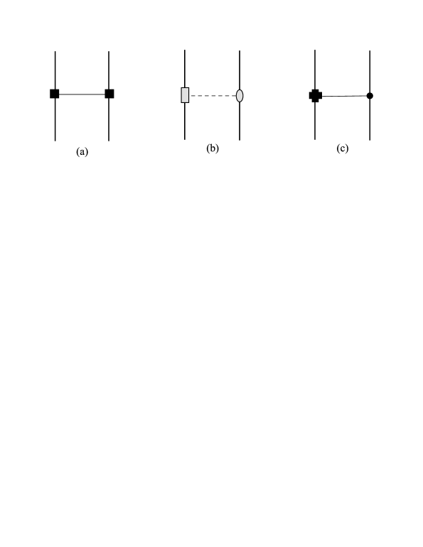
Figure 3: LO quartic in spin interaction Feynman diagrams. Diagrams b and c here should be included together with their mirror images. On the left and right we have the quadrupole-quadrupole and hexadecapole-monopole interactions, each of which is analogous to the LO spin-squared interaction in figure 1 here. On the middle we have the octupole-dipole interaction analogous to the LO spin1-spin2 interaction in figure 1 of Levi:2008nh .

Hence, the values of the Feynman diagrams of the LO quartic in spin interaction are given by the following:

$$\text{Fig.~{}3(a)}= \frac{3}{4}C_{1\text{(ES${}^{2}$)}}C_{2(\text{ES${}^{2}$)}}\frac{G}{m_{1}m_{2}r^{5}}\left[S_{1}^{2}S_{2}^{2}+2\left(\vec{S}_{1}\cdot\vec{S}_{2}\right)^{2}-5\left(S_{1}^{2}\left(\vec{S}_{2}\cdot\vec{n}\right)^{2}\right.\right.$$

$$\qquad\qquad\qquad\left.\left.+S_{2}^{2}\left(\vec{S}_{1}\cdot\vec{n}\right)^{2}+4\vec{S}_{1}\cdot\vec{S}_{2}\,\vec{S}_{1}\cdot\vec{n}\,\vec{S}_{2}\cdot\vec{n}-7\left(\vec{S}_{1}\cdot\vec{n}\right)^{2}\left(\vec{S}_{2}\cdot\vec{n}\right)^{2}\right)\right],$$ (42)

$$\text{Fig.~{}3(b)}= \frac{3}{2}C_{1\text{(BS${}^{3}$)}}\frac{G}{m_{1}^{2}r^{5}}\left[S_{1}^{2}\,\vec{S}_{1}\cdot\vec{S}_{2}-5S_{1}^{2}\,\vec{S}_{1}\cdot\vec{n}\,\vec{S}_{2}\cdot\vec{n}-5\vec{S}_{1}\cdot\vec{S}_{2}\left(\vec{S}_{1}\cdot\vec{n}\right)^{2}\right.$$

$$\qquad\qquad\qquad\qquad\left.+\frac{35}{3}\vec{S}_{2}\cdot\vec{n}\left(\vec{S}_{1}\cdot\vec{n}\right)^{3}\right],$$ (43)

$$\text{Fig.~{}3(c)}= \frac{3}{8}C_{1\text{(ES${}^{4}$)}}\frac{Gm_{2}}{m_{1}^{3}r^{5}}\left[S_{1}^{4}-10S_{1}^{2}\left(\vec{S}_{1}\cdot\vec{n}\right)^{2}+\frac{35}{3}\left(\vec{S}_{1}\cdot\vec{n}\right)^{4}\right].$$ (44)

Here too the evaluation of the diagrams is straightforward. Moreover, we have no additions to the effective potential.

4.2 Effective potential and Hamiltonian

Summing all diagrams in figure 3, we get the following effective potential for the complete LO quartic in spin interaction:

$$V_{\text{SSSS}}^{\text{LO}}= -\frac{3}{4}C_{1\text{(ES${}^{2}$)}}C_{2\text{(ES${}^{2}$)}}\frac{G}{m_{1}m_{2}r^{5}}\left[S_{1}^{2}S_{2}^{2}+2\left(\vec{S}_{1}\cdot\vec{S}_{2}\right)^{2}-5\left(S_{1}^{2}\left(\vec{S}_{2}\cdot\vec{n}\right)^{2}\right.\right.$$

$$\qquad\qquad\qquad\quad\left.\left.+S_{2}^{2}\left(\vec{S}_{1}\cdot\vec{n}\right)^{2}+4\vec{S}_{1}\cdot\vec{S}_{2}\,\vec{S}_{1}\cdot\vec{n}\,\vec{S}_{2}\cdot\vec{n}-7\left(\vec{S}_{1}\cdot\vec{n}\right)^{2}\left(\vec{S}_{2}\cdot\vec{n}\right)^{2}\right)\right]$$

$$-\frac{3}{2}C_{1\text{(BS${}^{3}$)}}\frac{G}{m_{1}^{2}r^{5}}\left[S_{1}^{2}\,\vec{S}_{1}\cdot\vec{S}_{2}-5S_{1}^{2}\,\vec{S}_{1}\cdot\vec{n}\,\vec{S}_{2}\cdot\vec{n}-5\vec{S}_{1}\cdot\vec{S}_{2}\left(\vec{S}_{1}\cdot\vec{n}\right)^{2}\right.$$

$$\qquad\qquad\qquad\qquad\left.+\frac{35}{3}\vec{S}_{2}\cdot\vec{n}\left(\vec{S}_{1}\cdot\vec{n}\right)^{3}\right]+1\longleftrightarrow 2$$

$$-\frac{3}{8}C_{1\text{(ES${}^{4}$)}}\frac{Gm_{2}}{m_{1}^{3}r^{5}}\left[S_{1}^{4}-10S_{1}^{2}\left(\vec{S}_{1}\cdot\vec{n}\right)^{2}+\frac{35}{3}\left(\vec{S}_{1}\cdot\vec{n}\right)^{4}\right]+1\longleftrightarrow 2.$$ (45)

Here too, for black holes the new Wilson coefficient $C_{\text{ES}^{4}}$ can be fixed from the gauge invariant binding energy in Steinhoff:2012rw , which also checks our result in the small mass ratio case. From this we find that $C_{\text{ES}^{4}}=1$ for black holes.

We proceed to compare our effective potential with the ADM Hamiltonian results for a black hole binary in Hergt:2007ha ; Hergt:2008jn . However, it was found in Steinhoff:2012rw , that the black hole binary Hamiltonian at quartic order in each of the spins, which was derived in Hergt:2008jn , must be incomplete. Indeed, at leading order the source part of the Hamilton constraint $\mathcal{H}^{\text{matter}}$ is the source of the Newtonian potential, which corresponds to the NRG scalar field $\phi$. From eq. (26) we therefore expect a contribution to the Hamilton constraint of the form:

$$\mathcal{H}^{\text{matter}}_{\text{hexadecapole}}=\frac{C_{ES^{4}}}{24m^{3}}S^{i}S^{j}S^{k}S^{l}\partial_{i}\partial_{j}\partial_{k}\partial_{l}\delta.$$ (46)

Indeed, this term was not considered in Hergt:2008jn . The resulting contribution to the Hamiltonian is identical to the value of figure 3(c) up to an overall sign. Hence, we see that the conclusions of section VI and in particular eq. (6.5) in Hergt:2008jn are incorrect.

Collecting the pieces from eqs. (124), (131) in Hergt:2007ha , and taking into account our correction to eq. (6.5) in Hergt:2008jn , that we just noted in eq. (46), coming from the hexadecapole-monopole interaction in fig. 3(c) here (for $C_{\text{ES}^{4}}=1$), we obtain the complete correct binary black hole ADM Hamiltonian:

$$H_{\text{SSSS(BHB)}}^{\text{LO}} =-\frac{3}{2}\frac{G}{m_{1}m_{2}r^{5}}\left[\frac{1}{2}\vec{S}_{1}^{2}\vec{S}_{2}^{2}+\left(\vec{S}_{1}\!\cdot\!\vec{S}_{2}\right)^{2}-\frac{5}{2}\left(\vec{S}_{1}^{2}\left(\vec{S}_{2}\!\cdot\!\vec{n}\right)^{2}+\vec{S}_{2}^{2}\left(\vec{S}_{1}\!\cdot\!\vec{n}\right)^{2}\right)\right.$$

$$\left.\qquad\qquad\qquad-10\vec{S}_{1}\!\cdot\!\vec{n}\,\vec{S}_{2}\!\cdot\!\vec{n}\left(\vec{S}_{1}\!\cdot\!\vec{S}_{2}-\frac{7}{4}\vec{S}_{1}\!\cdot\!\vec{n}\,\vec{S}_{2}\!\cdot\!\vec{n}\right)\right]$$

$$\quad-\frac{3}{2}\frac{G}{m_{1}^{2}r^{5}}\left[\vec{S}_{1}^{2}\,\vec{S}_{1}\!\cdot\!\vec{S}_{2}-5\vec{S}_{1}\!\cdot\!\vec{S}_{2}\left(\vec{S}_{1}\!\cdot\!\vec{n}\right)^{2}-5\vec{S}_{1}^{2}\,\vec{S}_{1}\!\cdot\!\vec{n}\,\vec{S}_{2}\!\cdot\!\vec{n}\right.$$

$$\qquad\qquad\qquad\qquad\quad+\frac{35}{3}\vec{S}_{2}\!\cdot\!\vec{n}\left(\vec{S}_{1}\!\cdot\!\vec{n}\right)^{3}\bigg{]}+1\longleftrightarrow 2$$

$$\quad-\frac{3Gm_{2}}{8m_{1}^{3}r^{5}}\left[S_{1}^{4}-10S_{1}^{2}\left(\vec{S}_{1}\cdot\vec{n}\right)^{2}+\frac{35}{3}\left(\vec{S}_{1}\cdot\vec{n}\right)^{4}\right]+1\longleftrightarrow 2.$$ (47)

With our correction included we then find full agreement of our result in eq. (4.2) with the black hole binary ADM Hamiltonian in eq. (4.2). Again, this comparison can also be used to fix $C_{\text{BS}^{3}}=1$ for the black hole case.

5 Conclusions

In this work we derived for the first time the complete LO cubic and quartic in spin interaction potentials for generic compact binaries via the effective field theory for gravitating spinning objects Levi:2015msa . These corrections, which enter at the 3.5PN and 4PN orders, respectively, for rapidly rotating compact objects, complete the LO finite size effects with spin up to the 4PN accuracy. In order to complete the spin dependent conservative sector to 4PN order, it remains to apply the effective field theory for gravitating spinning objects Levi:2015msa at NNLO to quadratic level in spin, which was initiated in Levi:2011eq .

We arrive at the results here by augmenting the effective action with new higher dimensional nonminimal coupling worldline operators, involving higher-order derivatives of the field, coupled to the higher-order multipole moments with spins, and introducing new Wilson coefficients, corresponding to constants, which describe the octupole and hexadecapole deformations of the object due to spin. These Wilson coefficients are fixed to unity in the black hole case via comparisons with the gauge invariant binding energy in the test particle limit and with the ADM Hamiltonian. We also see that the ADM Hamiltonian result for the quartic in spin interaction potential for a black hole binary, which was derived in Hergt:2008jn , is incorrect, and we complete this result.

It should be noted that the relation between the Wilson coefficients in this work and the multipole moments used in numerical codes, e.g. Laarakkers:1997hb ; Pappas:2012ns ; Yagi:2014bxa , and the Geroch-Hansen multipoles for black holes noted in eq. (37), should be worked out via a formal EFT matching procedure. Clearly, this involves subtleties Pappas:2012ns , and is left for future research. Yet we also note that recently, universal relations, nearly equation-of-state independent, were found between certain neutron star observables Yagi:2013bca ; Yagi:2013awa . It was demonstrated in Yagi:2014bxa , that all multipoles seem to be related in an approximately universal manner, though the accuracy of this approximation becomes worse for higher multipoles. This implies a universal relation between the coefficients $C_{ES^{2}}$, $C_{BS^{3}}$, and $C_{ES^{4}}$ in our potentials also for neutron stars. Thus, the new potentials effectively do not introduce new parameters. This is important for gravitational wave experiments, since a larger parameter space would render the parameter estimation more difficult. Instead, our potentials essentially just refine the precision of the equations of motion or of the binding energy without enlarging the parameter space.

The nonminimal coupling worldline operators enter the point particle action with the electric and magnetic components of the Weyl tensor of even and odd parity, coupled to the even and odd worldline spin tensors, respectively. Moreover, the NRG field decomposition, which we employ, demonstrates a coupling hierarchy of the gravito-magnetic vector and the Newtonian scalar to the odd and even in spin operators, respectively, which extends that of minimal coupling. Therefore the NRG fields are found to be very useful for the treatment of interactions involving spins, since they also facilitate the construction of the Feynman diagrams, and provide here instructive analogies between the LO spin-orbit and cubic in spin interactions, and between the LO quadratic and quartic in spin interactions. These analogies are based on the correspondence between the even and odd parity multipole moments with spin.

Finally, we note that we see that beyond the LO finite size effect with spin, namely the LO spin-squared interaction, which is a purely Newtonian effect, all LO finite size effects with spin are relativistic ones.

Note added.

After the preprint of this work has appeared, there appeared two related works: One work Vaidya:2014kza recovered specific pieces of the LO cubic and quartic in spin Hamiltonians from the S-matrix combined with EFT techniques; Another work Marsat:2014xea computed LO cubic in spin effects at the level of the EOM, and at the energy flux, via traditional methods. Both works found agreement with our results.

References

- (1) “LIGO webpage.” http://www.ligo.caltech.edu.
- (2) “Virgo webpage.” https://wwwcascina.virgo.infn.it.
- (3) “KAGRA webpage.” http://gwcenter.icrr.u-tokyo.ac.jp/en.
- (4) L. Blanchet, Gravitational Radiation from Post-Newtonian Sources and Inspiralling Compact Binaries, Living Rev.Rel. 17 (2014) 2, [arXiv:1310.1528].
- (5) K. Yagi and N. Yunes, Love can be Tough to Measure, Phys.Rev. D89 (2014) 021303, [arXiv:1310.8358].
- (6) J. E. McClintock, R. Narayan, S. W. Davis, L. Gou, A. Kulkarni, et al., Measuring the Spins of Accreting Black Holes, Class.Quant.Grav. 28 (2011) 114009, [arXiv:1101.0811].
- (7) T. Damour, P. Jaranowski, and G. Schäfer, Nonlocal-in-time action for the fourth post-Newtonian conservative dynamics of two-body systems, Phys.Rev. D89 (2014) 064058, [arXiv:1401.4548].
- (8) P. D. D’Eath, Interaction of two black holes in the slow-motion limit, Phys.Rev. D12 (1975) 2183–2199.
- (9) K. S. Thorne and J. B. Hartle, Laws of motion and precession for black holes and other bodies, Phys.Rev. D31 (1985) 1815–1837.
- (10) B. Barker and R. O’Connell, Gravitational Two-Body Problem with Arbitrary Masses, Spins, and Quadrupole Moments, Phys.Rev. D12 (1975) 329–335.
- (11) E. Poisson, Gravitational waves from inspiraling compact binaries: The Quadrupole moment term, Phys.Rev. D57 (1998) 5287–5290, [gr-qc/9709032].
- (12) R. A. Porto and I. Z. Rothstein, Next to Leading Order Spin(1)Spin(1) Effects in the Motion of Inspiralling Compact Binaries, Phys.Rev. D78 (2008) 044013, [arXiv:0804.0260]. [Erratum-ibid. D81 (2010) 029905].
- (13) J. Steinhoff, S. Hergt, and G. Schäfer, Spin-squared Hamiltonian of next-to-leading order gravitational interaction, Phys.Rev. D78 (2008) 101503, [arXiv:0809.2200].
- (14) S. Hergt and G. Schäfer, Higher-order-in-spin interaction Hamiltonians for binary black holes from Poincare invariance, Phys.Rev. D78 (2008) 124004, [arXiv:0809.2208].
- (15) S. Hergt, J. Steinhoff, and G. Schäfer, Reduced Hamiltonian for next-to-leading order Spin-Squared Dynamics of General Compact Binaries, Class.Quant.Grav. 27 (2010) 135007, [arXiv:1002.2093].
- (16) S. Hergt and G. Schäfer, Higher-order-in-spin interaction Hamiltonians for binary black holes from source terms of Kerr geometry in approximate ADM coordinates, Phys.Rev. D77 (2008) 104001, [arXiv:0712.1515].
- (17) J. Steinhoff and D. Puetzfeld, Influence of internal structure on the motion of test bodies in extreme mass ratio situations, Phys.Rev. D86 (2012) 044033, [arXiv:1205.3926].
- (18) M. Levi and J. Steinhoff, An effective field theory for gravitating spinning objects in the post-Newtonian scheme, arXiv:1501.04956.
- (19) W. D. Goldberger and I. Z. Rothstein, An Effective field theory of gravity for extended objects, Phys.Rev. D73 (2006) 104029, [hep-th/0409156].
- (20) W. D. Goldberger, Les Houches lectures on effective field theories and gravitational radiation, hep-ph/0701129.
- (21) R. A. Porto, Post-Newtonian corrections to the motion of spinning bodies in NRGR, Phys.Rev. D73 (2006) 104031, [gr-qc/0511061].
- (22) B. Kol and M. Smolkin, Non-Relativistic Gravitation: From Newton to Einstein and Back, Class.Quant.Grav. 25 (2008) 145011, [arXiv:0712.4116].
- (23) B. Kol, M. Levi, and M. Smolkin, Comparing space+time decompositions in the post-Newtonian limit, Class.Quant.Grav. 28 (2011) 145021, [arXiv:1011.6024].
- (24) M. Levi, Next to Leading Order gravitational Spin1-Spin2 coupling with Kaluza-Klein reduction, Phys.Rev. D82 (2010) 064029, [arXiv:0802.1508].
- (25) M. Levi, Next to Leading Order gravitational Spin-Orbit coupling in an Effective Field Theory approach, Phys.Rev. D82 (2010) 104004, [arXiv:1006.4139].
- (26) M. Levi, Binary dynamics from spin1-spin2 coupling at fourth post-Newtonian order, Phys.Rev. D85 (2012) 064043, [arXiv:1107.4322].
- (27) D. Bini, T. Damour, and G. Faye, Effective action approach to higher-order relativistic tidal interactions in binary systems and their effective one body description, Phys.Rev. D85 (2012) 124034, [arXiv:1202.3565].
- (28) A. J. Hanson and T. Regge, The Relativistic Spherical Top, Annals Phys. 87 (1974) 498.
- (29) I. Bailey and W. Israel, Lagrangian Dynamics of Spinning Particles and Polarized Media in General Relativity, Commun.Math.Phys. 42 (1975) 65–82.
- (30) T. Damour and G. Schäfer, Redefinition of position variables and the reduction of higher order Lagrangians, J.Math.Phys. 32 (1991) 127–134.
- (31) M. Levi and J. Steinhoff, Equivalence of ADM Hamiltonian and Effective Field Theory approaches at next-to-next-to-leading order spin1-spin2 coupling of binary inspirals, JCAP 1412 (2014) 003, [arXiv:1408.5762].
- (32) R. Hansen, Multipole moments of stationary space-times, J.Math.Phys. 15 (1974) 46–52.
- (33) F. Ryan, Gravitational waves from the inspiral of a compact object into a massive, axisymmetric body with arbitrary multipole moments, Phys.Rev. D52 (1995) 5707–5718.
- (34) W. G. Laarakkers and E. Poisson, Quadrupole moments of rotating neutron stars, Astrophys.J. 512 (1999) 282–287, [gr-qc/9709033].
- (35) G. Pappas and T. A. Apostolatos, Revising the multipole moments of numerical spacetimes, and its consequences, Phys.Rev.Lett. 108 (2012) 231104, [arXiv:1201.6067].
- (36) K. Yagi, K. Kyutoku, G. Pappas, N. Yunes, and T. A. Apostolatos, Effective No-Hair Relations for Neutron Stars and Quark Stars: Relativistic Results, Phys.Rev. D89 (2014) 124013, [arXiv:1403.6243].
- (37) K. Yagi and N. Yunes, I-Love-Q, Science 341 (2013) 365–368, [arXiv:1302.4499].
- (38) K. Yagi and N. Yunes, I-Love-Q Relations in Neutron Stars and their Applications to Astrophysics, Gravitational Waves and Fundamental Physics, Phys.Rev. D88 (2013) 023009, [arXiv:1303.1528].
- (39) V. Vaidya, Gravitational spin Hamiltonians from the S matrix, Phys.Rev. D91 (2015) 024017, [arXiv:1410.5348].
- (40) S. Marsat, Cubic order spin effects in the dynamics and gravitational wave energy flux of compact object binaries, arXiv:1411.4118.