Transmit without Regrets: Online Optimization in MIMO–OFDM Cognitive Radio Systems

Abstract

In this paper, we examine cognitive radio systems that evolve dynamically over time due to changing user and environmental conditions. To combine the advantages of orthogonal frequency division multiplexing (OFDM) and multiple-input, multiple-output (MIMO) technologies, we consider a MIMO–OFDM cognitive radio network where wireless users with multiple antennas communicate over several non-interfering frequency bands. As the network’s primary users (PUs) come and go in the system, the communication environment changes constantly (and, in many cases, randomly). Accordingly, the network’s unlicensed, secondary users (SUs) must adapt their transmit profiles “on the fly” in order to maximize their data rate in a rapidly evolving environment over which they have no control. In this dynamic setting, static solution concepts (such as Nash equilibrium) are no longer relevant, so we focus on dynamic transmit policies that lead to no regret: specifically, we consider policies that perform at least as well as (and typically outperform) even the best fixed transmit profile in hindsight. Drawing on the method of matrix exponential learning and online mirror descent techniques, we derive a no-regret transmit policy for the system’s SUs which relies only on local channel state information (CSI). Using this method, the system’s SUs are able to track their individually evolving optimum transmit profiles remarkably well, even under rapidly (and randomly) changing conditions. Importantly, the proposed augmented exponential learning (AXL) policy leads to no regret even if the SUs’ channel measurements are subject to arbitrarily large observation errors (the imperfect CSI case), thus ensuring the method’s robustness in the presence of uncertainties.

I Introduction

The explosive spread of Internet-enabled mobile devices has turned the radio spectrum into a scarce resource which, if not managed properly, may soon be unable to accommodate the soaring demand for wireless broadband and the ever-growing volume of data traffic and cellphone calls. Exacerbating this issue, studies by the US Federal Communications Commission (FCC) and the National Telecommunications and Information Administration (NTIA) have shown that this vital commodity is effectively squandered through underutilization and inefficient use: only $15\%$ to $85\%$ of the licensed radio spectrum is used on average, leaving ample spectral voids that could be exploited for opportunistic radio access [1, 2].

In view of the above, the emerging paradigm of cognitive radio (CR) has attracted considerable interest as a promising counter to spectrum scarcity [3, 4, 5, 6]. At its core, this paradigm is simply a two-level hierarchy between communicating users based on spectrum licensing. On the one hand, the network’s primary users have purchased spectrum rights but allow others to access it provided that their negotiated quality of service (QoS) guarantees are not violated; on the other hand, the network’s secondary users are free-riding on the licensed part of the spectrum, but they have no QoS guarantees and must conform to the constraints imposed by the PUs. In this way, by opening up the unfilled “white spaces” of the licensed spectrum to opportunistic radio access, the overall utilization of the wireless medium can be greatly increased without compromising the performance guarantees that the network’s licensed users have already paid for.

Orthogonally to the above, the seminal prediction that multiple-input and multiple-output (MIMO) technologies can lead to substantial gains in information throughput [7, 8] opens up additional ways for overcoming spectrum scarcity. In particular, by employing multiple antennas, it is possible to exploit spatial degrees of freedom in the transmission and reception of radio signals, the only physical limit being the number of antennas that can be deployed on a portable device. As a result, the existing wireless medium can accommodate greater volumes of data traffic per Hertz without requiring the reallocation (and subsequent re-regulation) of additional frequency bands.

In this paper, we combine these two approaches and focus on dynamic MIMO cognitive radio systems comprising several wireless users (primary and secondary alike) who communicate over multiple non-interfering channels. In this evolving (and unregulated) context, the intended receiver of a message has to cope with unwarranted interference from a large number of transmitters, a factor which severely limits the capacity of the wireless system in question. As a result, given that the system’s SUs cannot rely on contractual QoS guarantees to achieve their desired throughput levels, the maximization of their achievable transmission rates under the operational constraints imposed by the network’s PUs becomes a critical issue.

On that account, and given that the theoretical performance limits of MIMO systems still elude us (even in basic network models such as the interference channel), a widespread approach is to treat the interference from other users as additive colored noise and to use the mutual information for Gaussian input and noise as a unilateral performance metric [8]. However, since users cannot be assumed to have full information on the wireless system as it evolves over time (due to the arrival of new users, fluctuations in the PUs’ demand, etc.), they must optimize their signal characteristics “on the fly”, based only on locally available information. Hence, our aim is to derive a dynamic transmit policy that allows the system’s SUs to adapt to changes in the wireless medium and to track their individually optimum transmission profiles using only local (and possibly imperfect) channel state information (CSI).

This setting is fairly general and involves cognitive SUs with significant control over both spatial (MIMO) and spectral ( orthogonal frequency division multiplexing (OFDM)) degrees of freedom. To the best of our knowledge, only special cases of this problem have been considered in a CR setting. For instance, [9, 10, 11] analyzed the case where there is only one channel and the environment is static (i.e. the system’s SUs only react to each other and the PUs’ spectrum utilization is fixed); in this context, [9] characterized the best spatial covariance profile for the interacting SUs whereas [10, 11] described how to reach a Nash equilibrium in the resulting non-cooperative game. On the other hand, the authors of [12, 13, 14, 15] proposed different learning schemes for optimal channel selection in dynamic environments where the PUs’ evolving behavior cannot be anticipated by the system’s SUs, but only in the case where the SUs are equipped with a single antenna and cannot split power across subcarriers.

Extending the above considerations, our goal in this paper is to derive an adaptive transmit policy for SU rate optimization in dynamically evolving MIMO–OFDM cognitive radio networks. In this online optimization framework, the most widely used performance criterion is that of regret minimization, a concept which was first introduced by Hannan [16] and which has since given rise to a vigorous literature at the interface of optimization, statistics, game theory, and machine learning – see e.g. [17, 18] for a comprehensive survey. Specifically, in the language of game theory, the notion of (external) regret compares the agent’s cumulative payoff over time to what he would have obtained by constantly playing the same action. Accordingly, the purpose of regret minimization is to devise learning policies that lead to vanishingly small regret against any fixed action and irrespective of how the agent’s environment evolves over time.

In view of the above, we will focus on no-regret policies that perform at least as well as the asymptotically best fixed policy in terms of each user’s achievable transmission rate – despite the fact that the latter cannot be determined by the SUs when they have no means to anticipate the PUs’ behavior. In particular, motivated by the no-regret properties of the exponential weight (EW) algorithm for problems with discrete action sets [17, 19, 20, 21], we propose an augmented exponential learning (AXL) approach that can be applied to the continuous regret minimization problem at hand with minimal information requirements. A key challenge here is that any learning algorithm must respect the problem’s semidefiniteness constraints; as such, an important component of our AXL scheme is the continuous-time technique of matrix exponential learning that was recently introduced for ordinary (as opposed to online) rate optimization problems in MIMO multiple access channels [22] – and which is in turn closely related to the online mirror descent approach of [18] and the matrix regularization techniques of [23].

Of course, since the SUs’ optimal transmit profile varies over time, the notions of convergence and/or convergence speed are no longer applicable; instead, the figure of merit is the rate at which the SUs attain a no-regret state. In that respect, AXL guarantees a worst-case average regret of $\operatorname{\mathcal{O}}(T^{-1/2})$ after $T$ epochs, a bound which is well known to be tight [17, 18]. Additionally, AXL retains its no-regret properties even if the SUs’ channel measurements are subject to arbitrarily large observation errors (the imperfect CSI case), thus providing significant performance improvements over more traditional water-filling methods that are sensitive to perfect CSI. As a result, the system’s SUs are able to track their individually optimum transmit profile as it evolves over time remarkably well, even under rapidly (and randomly) changing conditions.

Paper Outline and Summary of Results

The breakdown of our paper is as follows: in Section II, we introduce our MIMO–OFDM cognitive radio network model and the notion of a no-regret transmission policy in the context of SU rate optimization. In Section III, we decompose this online rate optimization problem into two components, and we propose a no-regret algorithm for each one. Specifically, in Section III-A, we propose an adaptive power allocation policy for the problem’s OFDM component, whereas in Section III-B, we derive a dynamic signal covariance policy for the problem’s MIMO component based on matrix exponential learning. These components are fused in Section IV where we present our augmented exponential learning (AXL) method for the general MIMO-OFDM setting and we show that it leads to no regret (Theorem 1). Importantly, we also show that the AXL algorithm retains its no-regret properties even when the users only have imperfect CSI at their disposal (Theorem 2). This theoretical analysis is validated and supplemented by numerical simulations in Section V where we also examine the users’ ability to track their individually optimum transmit characteristics. To facilitate presentation, proofs and technical details have been delegated to a series of appendices at the end of the paper.

II System Model

II-A The Network Model

The cognitive radio system that we will focus on consists of a set of non-cooperative wireless MIMO users (primary and secondary alike) that communicate over several non-interfering subcarriers by means of an OFDM scheme [24, 25]. Specifically, let $\mathcal{Q}=\mathcal{P}\cup\mathcal{S}$ denote the set of the system’s users with $\mathcal{P}$ (resp. $\mathcal{S}$) representing the system’s primary (resp. secondary) users; assume further that each user $q\in\mathcal{Q}$ is equipped with $m_{q}$ transmit antennas and that the radio spectrum is partitioned into a set $\mathcal{K}=\{1,\dotsc,K\}$ of $K$ orthogonal frequency bands [24]. Then, the aggregate signal $\mathbf{y}_{k}^{s}\in\mathbb{C}^{n_{s}}$ on the $k$-th subcarrier at the intended receiver of the secondary user $s\in\mathcal{S}$ (assumed equipped with $n_{s}$ receive antennas) will be:

$$\mathbf{y}_{k}^{s}=\mathbf{H}_{k}^{ss}\mathbf{x}_{k}^{s}+\sum\nolimits_{p\in\mathcal{P}}\mathbf{H}_{k}^{ps}\mathbf{x}_{k}^{p}+\sum\nolimits_{r\in\mathcal{S},r\neq s}\mathbf{H}_{k}^{rs}\mathbf{x}_{k}^{r}+\mathbf{z}_{k}^{s},$$ (1)

where $\mathbf{x}_{k}^{q}\in\mathbb{C}^{m_{q}}$ is the transmitted message of user $q\in\mathcal{Q}$ (primary or secondary) over the $k$-th subcarrier, $\mathbf{H}_{k}^{qs}$ is the channel matrix between the $q$-th transmitter and the intended receiver of user $s$, and $\mathbf{z}_{k}^{s}\in\mathbb{C}^{n_{s}}$ is the noise in the channel, including thermal, atmospheric and other peripheral interference effects (and modeled as a non-singular, zero-mean Gaussian vector). Accordingly, if we focus for simplicity on a specific SU and drop the user index $s\in\mathcal{S}$ in (1), we obtain the signal model

$$\mathbf{y}_{k}=\mathbf{H}_{k}\mathbf{x}_{k}+\mathbf{w}_{k},$$ (2)

where $\mathbf{w}_{k}$ denotes the multi-user interference-plus-noise (MUI) over subcarrier $k\in\mathcal{K}$ at the intended receiver.

The covariance of $\mathbf{w}_{k}$ in (2) obviously changes over time due to fading, modulations in the PUs’ behavior, etc.; as a result, employing sophisticated successive interference cancellation (SIC) techniques at the receiver is highly nontrivial, especially with regards to the system’s unregulated secondary users; Instead, we will work in the single user decoding (SUD) regime where interference by other users (primary and secondary alike) is treated as additive, colored noise. In this context, the transmission rate of a user under the signal model (2) is given by the familiar expression [8, 24]:

$$\textstyle\Phi(\mathbf{P})=\sum\nolimits_{k}\big{[}\log\det\big{(}\mathbf{W}_{k}+\mathbf{H}_{k}\mathbf{P}_{k}\mathbf{H}_{k}^{{\dagger}}\big{)}-\log\det\mathbf{W}_{k}\big{]},$$ (3)

where:

1. $\mathbf{W}_{k}=\operatorname{\mathbb{E}}\big{[}\mathbf{w}_{k}\mathbf{w}_{k}^{{\dagger}}\big{]}$ is the multi-user interference-plus-noise covariance matrix over subcarrier $k$.

2. $\mathbf{P}_{k}=\operatorname{\mathbb{E}}[\mathbf{x}_{k}\mathbf{x}_{k}^{{\dagger}}]$ is the covariance matrix of the user’s transmitted signal on subcarrier $k$ and $\mathbf{P}=\operatorname{diag}(\mathbf{P}_{1},\dotsc,\mathbf{P}_{K})$ denotes the user’s transmit profile over all subcarriers. In particular, we will write for convenience:

   $$\mathbf{P}_{k}=p_{k}\mathbf{Q}_{k},$$ (4)

   where $p_{k}=\operatorname{\mathbb{E}}[\mathbf{x}_{k}^{{\dagger}}\mathbf{x}_{k}]$ denotes the user’s transmit power over subcarrier $k$ and $\mathbf{Q}_{k}=\operatorname{\mathbb{E}}\big{[}\mathbf{x}_{k}\mathbf{x}_{k}^{{\dagger}}\big{]}\big{/}\operatorname{\mathbb{E}}\big{[}\mathbf{x}_{k}^{{\dagger}}\mathbf{x}_{k}\big{]}$ is his normalized signal covariance matrix.

Hence, given that $\mathbf{W}_{k}$ may change over time due to evolving user conditions, we obtain the time-dependent objective:

$$\textstyle\Phi(\mathbf{P};t)=\sum\nolimits_{k}\log\det\big{[}\mathbf{I}+\widetilde{\mathbf{H}}_{k}(t)\,\mathbf{P}_{k}\,\widetilde{\mathbf{H}}_{k}^{{\dagger}}(t)\big{]},$$ (5)

where the effective channel matrices $\widetilde{\mathbf{H}}_{k}$ are given by

$$\widetilde{\mathbf{H}}_{k}(t)=\mathbf{W}_{k}(t)^{-1/2}\,\mathbf{H}_{k}(t),$$ (6)

and the time variable $t=1,2,\dotsc$ is assumed discrete (for instance, corresponding to the epochs of a time-slotted system).

Obviously, since we are putting no constraints on the behavior of the system’s users, the evolution of the effective channel matrices $\widetilde{\mathbf{H}}_{k}(t)$ over time can be quite arbitrary as well. Formally, we only make the following (minimal) assumptions:

1. The effective channel matrices $\widetilde{\mathbf{H}}_{k}(t)$ are bounded for all $t$.

2. The matrices $\widetilde{\mathbf{H}}_{k}(t)$ change sufficiently slowly relative to the coherence time of the channel so that the standard results of information theory [8] continue to hold.

3. SUs can obtain possibly imperfect (but otherwise unbiased) estimates for $\widetilde{\mathbf{H}}_{k}$, e.g. by measuring $\mathbf{H}_{k}$ and probing the intended receiver for the MUI covariance matrix $\mathbf{W}_{k}$.

In light of the above, and motivated by the “white-space filling” paradigm advocated (e.g. by the FCC) as a means to minimize interference by unlicensed users [2, 1, 26, 10, 27], we will consider the following constraints for the system’s SUs:

1. Bounded total transmit power:

   $$\textstyle\operatorname{tr}(\mathbf{P})=\sum\nolimits_{k}p_{k}\leq P.$$ (7a)

2. Constrained transmit power per subcarrier:

   $$\operatorname{tr}(\mathbf{P}_{k})=p_{k}\leq P_{k}.$$ (7b)

3. Null-shaping constraints:

   $$\mathbf{U}_{k}^{{\dagger}}\mathbf{P}_{k}=0,$$ (7c)

   for some tall complex matrix $\mathbf{U}_{k}$ with full column rank.

Of the constraints above, (7a) is a physical constraint on the user’s total transmit power, (7b) imposes a limit on the interference level that can be tolerated on a given subcarrier, and (7c) is a “hard”, spatial version of (7b) which guarantees that certain spatial dimensions per subcarrier are only open to licensed, primary users. In more detail, (7b) is equivalent to limiting the maximal average interference that SUs are allowed to incur on the primary transmission while the matrices $\mathbf{U}_{k}$ of (7c) are imposed by the PUs and their columns represent the spatial directions which are forbidden to SU transmission. Such constraints are well-documented in the literature and simply reflect the fact that some carriers or spatial directions per carrier are preferred by the PUs, so stricter constraints are imposed to limit interference by SUs (for a more detailed discussion, see e.g. [25, 10, 11] and references therein).

Of course, to maximize (5) in the absence of energy awareness considerations, the user must saturate his total power constraint (7a) by transmitting at the highest possible (total) power. Thus, the set of admissible transmit profiles for the rate function (5) may be expressed as:

$$\textstyle\mathcal{X}=\big{\{}\operatorname{diag}(\mathbf{P}_{1},\dotsc,\mathbf{P}_{K}):\;\mathbf{P}_{k}\in\mathbb{C}^{m_{k}\times m_{k}},\\ \textstyle\mathbf{P}_{k}\succcurlyeq 0,0\leq\operatorname{tr}(\mathbf{P}_{k})\leq P_{k}\text{ and }\sum\nolimits_{k}\operatorname{tr}(\mathbf{P}_{k})=P\big{\}},$$ (8)

where $m_{k}\equiv\operatorname{nullity}(\mathbf{U}_{k})$ is the number of spatial dimensions that are open to SUs on subcarrier $k$. Accordingly, writing $\mathbf{P}_{k}$ in the decoupled form $\mathbf{P}_{k}=p_{k}\mathbf{Q}_{k}$ as in (4), we obtain the decomposition $\mathcal{X}=\mathcal{X}_{0}\times\prod_{k}\mathcal{D}_{k}$ where

$$\textstyle\mathcal{X}_{0}=\left\{\mathbf{p}\in\mathbb{R}^{K}:\;0\leq p_{k}\leq P_{k},\,\sum\nolimits_{k}p_{k}=P\right\}$$ (9)

denotes the set of admissible power allocation vectors and

$$\mathcal{D}_{k}=\big{\{}\mathbf{Q}_{k}\in\mathbb{C}^{m_{k}\times m_{k}}:\;\mathbf{Q}_{k}\succcurlyeq 0,\operatorname{tr}(\mathbf{Q}_{k})=1\big{\}}$$ (10)

is the set of admissible normalized covariance matrices for subcarrier $k$. We thus obtain the online rate maximization problem:

maximize $$\textstyle\Phi(\mathbf{P};t)$$ (ORM)

subject to $$\begin{cases}\mathbf{P}=\operatorname{diag}(p_{1}\mathbf{Q}_{1},\dotsc,p_{K}\mathbf{Q}_{K}),\\ (p_{1},\dotsc,p_{K})\in\mathcal{X}_{0},\;\mathbf{Q}_{k}\in\mathcal{D}_{k}.\end{cases}$$

Remark 1.

In the following sections, we will need the derivatives of $\Phi$; to that end, some matrix calculus yields

$$\frac{\partial\Phi}{\partial\mathbf{P}_{k}^{\ast}}\equiv\mathbf{M}_{k}(t)=\widetilde{\mathbf{H}}_{k}^{{\dagger}}(t)\big{[}\mathbf{I}+\widetilde{\mathbf{H}}_{k}(t)\mathbf{P}_{k}\widetilde{\mathbf{H}}_{k}^{{\dagger}}(t)\big{]}^{-1}\widetilde{\mathbf{H}}_{k}(t),$$ (11)

where $\mathbf{P}_{k}^{\ast}$ denotes the complex conjugate of $\mathbf{P}_{k}$. Since the effective channel matrices $\widetilde{\mathbf{H}}_{k}(t)$ are assumed bounded for all $t$, the above shows that there exists some $M>0$ such that:

$$\|\mathbf{M}_{k}(t)\|\leq M\quad\text{for all $k\in\mathcal{K}$, $\mathbf{P}\in\mathcal{X}$, and for all $t\geq 0$.}$$ (12)

II-B Online Optimization and Regret Minimization

In our setting, there is no direct causal link between the PUs’ behavior and the choices of the SUs, so the rate function $\Phi$ may change arbitrarily over time. This leads to a “game against nature” which is played out as follows:

1. At each time slot $t=1,2\dotsc$, the agent (i.e. the focal SU) selects an action (transmit profile) $\mathbf{P}(t)\in\mathcal{X}$.

2. The agent’s payoff (transmission rate) $\Phi(\mathbf{P}(t);t)$ is determined by nature and/or the behavior of other users (via the effective channel matrices $\widetilde{\mathbf{H}}_{k}$).

3. The agent employs some decision rule (dynamic transmit policy) to pick a new transmit profile $\mathbf{P}(t+1)\in\mathcal{X}$ at stage $t+1$, and the process is repeated until transmission ends.

In this dynamic setting, static solution concepts are no longer applicable, so the most widely used optimization criterion is that of regret minimization, a long-term solution concept which was first introduced by Hannan [16] and which has since given rise to an extremely active field of research at the interface of optimization, statistics and theoretical computer science – see e.g. [17, 18] for a survey. Roughly speaking, the regret compares the payoff obtained by an agent that follows a dynamic policy to the payoff that he would have obtained by constantly choosing the same action over the entire transmission horizon. More precisely, the cumulative regret of the dynamic policy $\mathbf{P}(t)\in\mathcal{X}$ with respect to $\mathbf{P}_{0}\in\mathcal{X}$ is defined as:

$$\operatorname{Reg}_{T}(\mathbf{P}_{0})=\sum\nolimits_{t=1}^{T}\big{[}\Phi(\mathbf{P}_{0};t)-\Phi(\mathbf{P}(t);t)\big{]},$$ (13)

i.e. $\operatorname{Reg}_{T}(\mathbf{P}_{0})$ measures the cumulative transmission rate difference up to stage $T$ between a benchmark transmit profile $\mathbf{P}_{0}\in\mathcal{X}$ and the dynamic policy $\mathbf{P}(t)$. The user’s average regret then is $T^{-1}\operatorname{Reg}_{T}(\mathbf{P}_{0})$ and the goal of regret minimization is to devise a dynamic policy $\mathbf{P}(t)$ that leads to no regret, viz.

$$\limsup\limits_{T\to\infty}\frac{1}{T}\operatorname{Reg}_{T}(\mathbf{P}_{0})\leq 0,$$ (14)

for all $\mathbf{P}_{0}\in\mathcal{X}$ and irrespective of the evolution of the objective $\Phi(\cdot;t)$ over time. In other words, if we interpret $\lim_{T\to\infty}T^{-1}\sum_{t=1}^{T}\Phi(\mathbf{P}_{0};t)$ as the long-term average transmission rate of $\mathbf{P}_{0}$, (14) means that the average data rate of the dynamic transmit policy $\mathbf{P}(t)$ must be at least as good as that of any benchmark profile $\mathbf{P}_{0}\in\mathcal{X}$.

Remark 2.

Obviously, if the optimum transmit policy which maximizes (ORM) could be predicted at every stage $t=1,2,\dotsc$ in an oracle-like fashion, we would have $\operatorname{Reg}_{T}(\mathbf{P}_{0})\leq 0$ in (13) for all $\mathbf{P}_{0}\in\mathcal{X}$. Therfore, the requirement (14) is fundamental in the context of online optimization because negative regret is a key indicator of tracking the maximum of (ORM) as it evolves over time.

Remark 3.

In the machine learning literature, there exist other notions of regret (such as internal, swap or adaptive regret [28]) for studying online optimization problems in changing environment. Due to space limitations, we will focus our theoretical analysis on the external regret formulation (13) and we will rely on the numerical simulations of Section V to show how well our proposed dynamic policies track the evolving maximum of the rate maximization problem (ORM).

Remark 4.

If the channel matrices are drawn at each realization from an isotropic distribution [29], spreading power uniformly across carriers and antennas is the optimal choice when nature (including the network’s PUs) is actively choosing the worst possible channel realization for the transmitter [29]. A no-regret policy extends this “min-max” concept by ensuring that the policy’s achieved transmission rate is asymptotically as good as that of any fixed transmit profile, including obviously the uniform one as a special case where nature is actively playing against the transmitter – e.g. jamming.

III Power Allocation and Signal Covariance Optimization

To build intuition step-by-step, we will break up the online rate maximization problem (ORM) in simpler components and we will derive a no-regret transmit policy for each one based on an exponential learning principle. These policies will then be fused into an adaptive transmit policy for the full MIMO–OFDM problem in Section IV.

III-A The OFDM Component: Online Power Allocation

III-A1 A gentle start – the case $P_{k}\geq P$

For illustration purposes, we first examine the case where the power-per-channel constraints (7b) can be absorbed in the total power constraint (7a), i.e. $P_{k}\geq P$ for all $k\in\mathcal{K}$. Also, for scaling purposes, it will be more convenient to consider the normalized power variables

$$q_{k}=p_{k}/P.$$ (15)

With this in mind, if the normalized signal covariance profile $\mathbf{Q}=\operatorname{diag}(\mathbf{Q}_{1},\dotsc,\mathbf{Q}_{K})$ of the focal SU is kept fixed, we obtain the online power allocation problem:

maximize $$\textstyle\Phi(\mathbf{q};t),$$ (OPA)

subject to $$\mathbf{q}\in\Delta$$

where $\Delta=\big{\{}\mathbf{q}\in\mathbb{R}_{+}^{K}:\sum_{k=1}^{K}q_{k}=1\big{\}}$ denotes the set of feasible (normalized) power allocation profiles and we write $\Phi(\mathbf{q};t)$ to highlight the dependence of the rate function (5) on the normalized power allocation profile $\mathbf{q}\in\Delta$ (instead of $\mathbf{P}\in\mathcal{X}$).

A special case of this problem is when the user cannot split power across subcarriers and can only choose one channel on which to transmit. Essentially, this channel selection framework boils down to the famous “multi-armed bandit” problem of [30] (see e.g. [17, 18] for a review). As a result, much recent work on CR networks [13, 14, 15] has been focused on no-regret channel selection algorithms based on $Q$-learning [14] or upper confidence bound (UCB) techniques [13].

Unfortunately, these techniques are inherently discrete in nature, so it is not clear how to extend them to the continuous context of (OPA). Instead, motivated by the exponential weight algorithm introduced in [19, 20, 21] for sequence prediction, our approach consists of scoring each channel over time and then allocating power proportionally to the exponential of these scores. In particular, inspired by the analysis of [31], each channel will be scored by means of the marginal utilities:

$$v_{k}=\frac{\partial\Phi}{\partial q_{k}}=P\frac{\partial\Phi}{\partial p_{k}}=P\cdot\operatorname{tr}\big{[}\mathbf{M}_{k}\mathbf{Q}_{k}\big{]},$$ (16)

where $\mathbf{Q}_{k}\in\mathcal{D}_{k}$ is the user’s (fixed) covariance matrix and $\mathbf{M}_{k}$ is given by (11). We thus obtain the exponential learning power allocation policy:

$$y_{k}(t) =y_{k}(t-1)+v_{k}(t),$$ (XL-PA)

$$q_{k}(t+1) =\frac{\exp\big{(}\eta t^{-1/2}y_{k}(t)\big{)}}{\sum_{\ell}\exp\big{(}\eta t^{-1/2}y_{\ell}(t)\big{)}},$$

where $\eta>0$ is a learning rate parameter and the $\sqrt{t}$ factor has been included to moderate very sharp score differences.

Our first result is that (XL-PA) performs asymptotically as well as any fixed power allocation profile $\mathbf{q}_{0}\in\Delta$:

Proposition 1.

If $P_{k}\geq P$ for all $k\in\mathcal{K}$, the policy (XL-PA) leads to no regret. Specifically, for every $\mathbf{q}_{0}\in\Delta$, and independently of the system’s evolution over time, we have

$$\frac{1}{T}\operatorname{Reg}_{T}(\mathbf{q}_{0})\leq\frac{1}{\sqrt{T}}\left(\frac{\log K}{\eta}+4P^{2}M^{2}\eta\right),$$ (17)

with $M$ given by (12).

Proof:

See Appendices -A and -E. ∎

Remark 1.

The use of the marginal utilities (16) in the exponential learning policy (XL-PA) can be compared to the online gradient descent algorithm introduced in [32] where the learner tracks the gradient of his evolving objective and projects back to the problem’s feasible set when needed. We did not take such an approach because projections are numerically unstable [33] and can become quite costly from a computational standpoint (the problem’s constraints would have to be checked individually at every iteration). Nonetheless, the exponential approach of (XL-PA) has strong ties to the method of online mirror descent [18] which we discuss later.

III-A2 The general case

The dynamic power allocation policy (XL-PA) concerns the case where the power-per-channel constraints (7b) can be absorbed in the total power constraint (7a). Otherwise, if $P_{k}<P$ for some channel $k\in\mathcal{K}$ (e.g. if certain PUs have very low interference tolerance on their licensed channels), (XL-PA) cannot be employed “as is” because it does not respect the constraint $p_{k}\leq P_{k}$. When this is the case, the analysis of Appendix -B yields the modified policy:

$$y_{k}(t) =y_{k}(t-1)+v_{k}(t),$$ (XL-PA^′)

$$p_{k}(t+1) =P_{k}\left(1+\exp(\lambda-\eta t^{-1/2}y_{k})\right)^{-1}$$

where $\lambda>0$ is defined implicitly so that (7a) is satisfied:

$$\textstyle P=\sum_{k\in\mathcal{K}}P_{k}\left(1+\exp(\lambda-\eta t^{-1/2}y_{k})\right)^{-1}.$$ (18)

Just like (XL-PA), (XL-PA^′) exhibits exponential sensitivity to the scores $y_{k}$ modulo a normalization factor corresponding to the constraints (7a) and (7b). Since the RHS of (18) is strictly decreasing in $\lambda$, it is then easy to calculate the value of $\lambda$ itself, e.g. by performing a line search for $e^{\lambda}$ [33]. We thus get:

Proposition 2.

The policy (XL-PA^′) leads to no regret. In particular, for every $\mathbf{p}_{0}\in\mathcal{X}_{0}$, the user’s regret is bounded by

$$T^{-1}\operatorname{Reg}_{T}(\mathbf{p}_{0})\leq\operatorname{\mathcal{O}}\big{(}T^{-1/2}\big{)},$$ (19)

irrespective of the system’s evolution over time.

Proof:

See Appendix -B. ∎

Remark.

We should note here that (XL-PA^′) is not equivalent to (XL-PA) if $P_{k}\geq P$; instead, (XL-PA) should be viewed as a simpler alternative to (XL-PA^′) that can be employed whenever the maximum power-per-channel constraints (7b) can be subsumed in the total power constraint (7a). For convenience, we will present our results in the simpler case $P_{k}\geq P$ and we will rely on a series of remarks to translate these remarks to the regime $P_{k}<P$ (cf. Appendices -A and -B).

III-B The MIMO Component: Signal Covariance Optimization

If the user’s power allocation profile $\mathbf{p}=(p_{1},\dotsc,p_{K})$ remains fixed throughout the transmission horizon, (ORM) boils down to the online signal covariance optimization problem:

maximize $$\textstyle\Phi(\mathbf{Q};t),$$ (OCOV)

subject to $$\textstyle\mathbf{Q}_{k}\succcurlyeq 0,\;\operatorname{tr}(\mathbf{Q}_{k})=1,$$

where we now use the notation $\Phi(\mathbf{Q};t)$ to highlight the dependence of the user’s transmission rate (5) on the normalized covariance matrix $\mathbf{Q}=\operatorname{diag}(\mathbf{Q}_{1},\dotsc,\mathbf{Q}_{K})\in\mathcal{X}_{+}\equiv\prod_{k}\mathcal{D}_{k}$.

A key challenge in (OCOV) is that any learning algorithm must respect the problem’s (implicit) semidefiniteness constraints $\mathbf{Q}_{k}\succcurlyeq 0$. To that end, motivated by the analysis of [22] (see also the matrix regularization approach of [23]), we will consider the matrix exponential learning policy

$$\mathbf{Y}_{k}(t) =\mathbf{Y}_{k}(t-1)+\mathbf{V}_{k}(t),$$ (XL-COV)

$$\mathbf{Q}_{k}(t+1) =\frac{\exp\big{(}\eta t^{-1/2}\mathbf{Y}_{k}(t)\big{)}}{\operatorname{tr}\big{[}\exp\big{(}\eta t^{-1/2}\mathbf{Y}_{k}(t)\big{)}\big{]}},$$

where the matrix-valued gradient payoff $\mathbf{V}_{k}$ is defined as:

$$\mathbf{V}_{k}=\frac{\partial\Phi}{\partial\mathbf{Q}_{k}^{\ast}}=p_{k}\mathbf{M}_{k},$$ (20)

and $\mathbf{M}_{k}$ is given by (11). Intuitively, (XL-COV) reinforces the spatial directions that peform well by increasing the corresponding eigenvalues while the $t^{-1/2}$ factor keeps the eigenvalues of $\mathbf{Q}_{k}$ from approaching zero too fast [35]. Along these lines, our analysis in Appendix -C yields:

Proposition 3.

The dynamic transmit policy (XL-COV) leads to no regret in the online signal covariance optimization problem (OCOV). In particular, for every $\mathbf{Q}_{0}\in\mathcal{X}_{+}\equiv\prod_{k}\mathcal{D}_{k}$, and irrespective of the system’s evolution over time, we have:

$$\frac{1}{T}\operatorname{Reg}_{T}(\mathbf{Q}_{0})\leq\frac{1}{\sqrt{T}}\left(\frac{\sum_{k=1}^{K}\log m_{k}}{\eta}+4P^{2}M^{2}\eta\right),$$ (21)

where $m_{k}$ is the number of spatial degrees of freedom left open by the constraint (7c).

IV Learning in the Full MIMO–OFDM Problem

IV-A Augmented Exponential Learning

Based on the analysis of the previous section, we derive here a dynamic no-regret policy for the full MIMO–OFDM problem (ORM). Working for simplicity with the special case $P_{k}\geq P$, (XL-PA) and (XL-COV) yield the dynamic transmit policy:

Parameter: $\eta>0$.
Initialize: $t\leftarrow 0$; channel scores $y_{k}\leftarrow 0$, $\mathbf{Y}_{k}\leftarrow 0$.
Repeat

      $t\leftarrow t+1$;
foreach channel $k\in\mathcal{K}$ do

            set $\displaystyle\begin{cases}p_{k}\leftarrow P\exp\big{(}\eta t^{-1/2}y_{k}\big{)}\big{/}\sum_{\ell}\exp\big{(}\eta t^{-1/2}y_{\ell}\big{)};\\ \mathbf{Q}_{k}\leftarrow\exp\big{(}\eta t^{-1/2}\mathbf{Y}_{k}\big{)}\big{/}\operatorname{tr}\big{[}\exp\big{(}\eta t^{-1/2}\mathbf{Y}_{k}\big{)}\big{]};\end{cases}$

      foreach channel $k\in\mathcal{K}$ do

            measure $\mathbf{M}_{k}\leftarrow\widetilde{\mathbf{H}}_{k}^{{\dagger}}\big{[}\mathbf{I}+p_{k}\widetilde{\mathbf{H}}_{k}\mathbf{Q}_{k}\widetilde{\mathbf{H}}_{k}^{{\dagger}}\big{]}^{-1}\widetilde{\mathbf{H}}_{k}$;
update scores: $\displaystyle\begin{cases}y_{k}\leftarrow y_{k}+P\operatorname{tr}[\mathbf{M}_{k}\mathbf{Q}_{k}];\\ \mathbf{Y}_{k}\leftarrow\mathbf{Y}_{k}+p_{k}\mathbf{M}_{k};\end{cases}$

       until transmission ends.

Algorithm 1 Augmented Exponential Learning (AXL)

The augmented exponential learning (AXL) algorithm above will be our main focus, so a few remarks are in order:

Remark 1.

From an implementation point of view, AXL has the following desirable properties:

1. It is distributed: each SU only needs to update his individual transmit policy using local CSI (the matrices $\widetilde{\mathbf{H}}_{k}$).

2. It is asynchronous: there is no need for a global update timer to synchronize the system’s SUs.

3. It is stateless: the SUs do not need to know the state of the system (e.g. the network’s topology), and/or be aware of each other’s actions.

4. It is reinforcing: the SUs tend to increase their unilateral transmission rates.

Remark 2.

If the maximum power-per-channel constraints imposed on the network’s SUs do not satisfy the condition $P_{k}\geq P$ for all $k\in\mathcal{K}$, the power update step of AXL must be modified: specifically, the exponential allocation rule $p_{k}\leftarrow P\exp(\eta t^{-1/2}y_{k})\big{/}\sum_{\ell}\exp(\eta t^{-1/2}y_{\ell})$ must be replaced by the update rule of (XL-PA^′), i.e. by setting $p_{k}\leftarrow P_{k}\big{[}1+\exp(\lambda-\eta t^{-1/2}y_{k})\big{]}^{-1}$. To simplify our presentation, we will keep the assumption $P_{k}\geq P$ with the implicit understanding that if $P_{k}<P$ for some $k\in\mathcal{K}$, then it is the modified version of AXL that should be used instead.

With all this in mind, our main result is that the AXL algorithm leads to no regret if $P_{k}\geq P$ for all channels:

Theorem 1.

The adaptive transmit policy generated by AXL leads to no regret in the online rate maximization problem (ORM). In particular, for every fixed transmit profile $\mathbf{P}_{0}\in\mathcal{X}$, and independently of how the system’s rate function (5) evolves over time, the user’s regret is bounded by:

$$\frac{1}{T}\operatorname{Reg}_{T}(\mathbf{P}_{0})\leq\frac{1}{\sqrt{T}}\left(\frac{\log K+\sum\nolimits_{k=1}^{K}\log m_{k}}{\eta}+4P^{2}M^{2}\eta\right),$$ (22)

where $M$ is given by (12) and $m_{k}$ is the number of spatial dimensions that are left open to SUs by the constraint (7c).

Proof:

See Appendices -D and -E. ∎

Remark 1.

As we already explained, if $P_{k}<P$ for some $k\in\mathcal{K}$, the power update step in the AXL algorithm should be replaced by the power allocation rule (XL-PA^′). In this case, AXL still guarantees an $\operatorname{\mathcal{O}}(T^{-1/2})$ regret bound but the exact expression is more complicated (see Appendix -B for the details).

Remark 2.

The proof of Theorem 1 relies on a deep connection between (XL-PA) and (XL-COV) with the Gibbs–Shannon and von Neumann entropy functions respectively. In fact, as we shall see in Appendices -A–-B, our approach is intimately related to the Hessian–Riemannian optimization method of [36] and the online mirror descent techniques of [18, 23]. Unfortunately, a full description of these methods requires the introduction of significant technical apparatus, so we will not discuss them at length; for a detailed account, the reader is instead referred to [18, 35].

Remark 3.

It should also be noted that the bound (22) is not the sum of the bounds (17) and (21). As we show in Appendices -D and -E, the reason for this is that Theorem 1 is not a corollary of Propositions 1 and 3 but, rather, a combination of these two independent results.

Remark 4.

In practice, the learning parameter $\eta$ of the AXL algorithm can be tuned freely by the user. As such, if the user can estimate ahead of time the quantity $M$ (which can be seen as an effective bound on the gradient matrices $\mathbf{M}_{k}$ over time), $\eta$ can be chosen so as to optimize the regret guarantee (22) – thus leading to lower regret levels faster. Specifically, some calculations along the lines of [35] show that the optimal choice of $\eta$ which minimizes the RHS of (22) is:

$$\textstyle\eta=\frac{1}{2}PM\left(\log K+\sum\nolimits_{k}\log m_{k}\right)^{1/2},$$ (23)

which then leads to the optimized regret guarantee:

$$\textstyle\operatorname{Reg}_{T}(\mathbf{P}_{0})\leq 4PM\big{(}\log K+\sum\nolimits_{k}\log m_{k}\big{)}^{1/2}T^{1/2}.$$ (24)

This bound resembles the bound derived in [23] for learning processes that stop after a predetermined number of steps; that being said (and in contrast to Theorem 1), unless some sort of “doubling correction” is used [17], the method proposed in [23] may lead to positive regret in an infinite horizon setting (such as the one we are considering here). On the other hand, this also shows that if the user can estimate his transmission horizon in advance (instead of having an infinite backlog of data to transmit), then he can use AXL with constant parameter $\eta$ given by (23) and still enjoy the optimal regret guarantee (24).

Remark 5.

Finally, we note that the optimal bound (24) is asymptotically tight with respect to $T$ but not necessarily with respect to the dimensionality of the problem. In particular, the analysis of [17, 18] shows that the best bound that can be guaranteed against an adversarial nature is $\operatorname{\mathcal{O}}(\sqrt{T})$; furthermore, if the state space of the problem is a simplex of dimension $K$, the tightest possible bound is $\operatorname{\mathcal{O}}(\log K)$ [17]. In this way, the $\log K$ factor of (24) is tight; we conjecture that the same holds for the $\log m_{k}$ factors because the covariance spectrahedrons $\mathcal{D}_{k}$ are simply the product of a simplex with dimension $m_{k}$ with the space of unitary matrices. At any rate, the bound (24) only tightens against an adversarial nature, so, in practical situations, we expect the user’s regret to decay much more rapidly (cf. the numerical simulations of Section V).

IV-B Learning with Imperfect Channel State Information

In practice, a major challenge occurs if the user does not have perfect CSI with which to calculate the matrix gradients (11) that are needed to run the AXL algorithm. To wit, since these gradients are determined by the effective channel matrices $\widetilde{\mathbf{H}}_{k}=\mathbf{W}_{k}^{-1/2}\mathbf{H}_{k}$, imperfect measurements of the actual channel matrices $\mathbf{H}_{k}$ or of the multi-user interference-plus-noise covariance matrices $\mathbf{W}_{k}$ would invariably interfere with each update cycle. Accordingly, our aim in this section is to study the robustness of AXL in the presence of measurement errors.

To account for as wide a range of errors as possible, we will assume that at each update period $t=1,2,\dotsc$, the user can only observe a noisy estimate

$$\hat{\mathbf{M}}_{k}(t)=\mathbf{M}_{k}(t)+\mathbf{\Xi}_{k}(t)$$ (25)

of $\mathbf{M}_{k}(t)$, where the noise process $\mathbf{\Xi}_{k}(t)$ represents a random and unbiased observational error (not necessarily i.i.d.). Formally:

Assumption 1.

We assume that the observation error $\mathbf{\Xi}_{k}$ is:

1. Bounded: $\|\mathbf{\Xi}_{k}(t)\|\leq\Sigma$ (a.s.) for some $\Sigma>0$ and for all $t$.

2. Unbiased: $\operatorname{\mathbb{E}}\big{[}\mathbf{\Xi}_{k}(t)|\mathcal{F}_{t-1}\big{]}=0$ where $\mathcal{F}=\{\mathcal{F}_{t}\}_{t\geq 1}$ denotes the history of the user’s choices.

Remarkably, as long as there is no systematic bias in the user’s measurements, the AXL algorithm still leads to no regret, even in the presence of arbitrarily large observation errors:

Theorem 2.

The AXL algorithm with noisy observations $\hat{\mathbf{M}}_{k}$ of the form (25) leads to no regret (a.s.). Specifically, if $\|\mathbf{\Xi}_{k}\|\leq\Sigma$, then, for all $\mathbf{P}_{0}\in\mathcal{X}$ and for all $z>0$:

1. The user’s expected regret is bounded by:

   $$\operatorname{\mathbb{E}}\left[T^{-1}\operatorname{Reg}_{T}(\mathbf{P}_{0})\right]\leq RT^{-1/2}.$$ (26)

2. The user’s realized regret is bounded by the perfect CSI guarantee of AXL with exponentially high probability:

   $$\operatorname{\mathbb{P}}\left(\frac{1}{T}\operatorname{Reg}_{T}(\mathbf{P}_{0})\leq\frac{R}{\sqrt{T}}+z\right)\geq 1-\exp\left(-\frac{z^{2}T}{2D^{2}\Sigma^{2}}\right),$$ (27)

where $D>0$ is a constant and $R$ is the deterministic guarantee (22) of AXL under perfect CSI, viz.:

$$\textstyle R=\eta^{-1}\cdot\big{(}\log K+\sum\nolimits_{k}\log m_{k}\big{)}+4P^{2}M^{2}\eta.$$ (28)

Theorem 2 (proven in Appendix -F) shows that AXL guarantees an $\operatorname{\mathcal{O}}(T^{-1/2})$ bound on the user’s regret with high probability, even under measurement errors of arbitrarily high magnitude. Accordingly, a few remarks are in order:

Remark 1.

The first- and second-order statistics of the measured gradients $\hat{\mathbf{M}}_{k}$ play different roles in the presence of imperfect CSI: the expected value $\operatorname{\mathbb{E}}\big{[}\hat{\mathbf{M}}_{k}\big{]}=\mathbf{M}_{k}$ of $\hat{\mathbf{M}}_{k}$ controls the expected regret guarantee of AXL via (26), whereas the variance $\operatorname{Var}\big{(}\hat{\mathbf{M}}_{k}\big{)}=\operatorname{\mathbb{E}}\big{[}\|\mathbf{\Xi}_{k}\|^{2}\big{]}$ of $\hat{\mathbf{M}}_{k}$ controls the deviations of the regret from its “bulk” behavior – but has no impact on the expected regret of AXL.

Remark 2.

Note also that Theorem 1 is recovered by (27) in the deterministic limit $\Sigma\to 0^{+}$: the probability that the user’s regret exceeds the determinstic guarantee $R/\sqrt{T}$ converges uniformly to $0$ as $\Sigma\to 0^{+}$.

V Numerical Results

To validate the predictions of Section IV for the AXL algorithm, we conducted extensive numerical simulations from which we illustrate here a selection of the most representative scenarios – though the observations made below remain valid in most typical mobile wireless environments.

In Fig. 1, we simulated a network consisting of $10$ PUs and $40$ SUs, all equipped with $m_{k}=3$ transmit/receive antennas, and communicating over $K=256$ orthogonal subcarriers with a base frequency of $\nu=2\,\mathrm{GHz}$. Both the PUs and the SUs were assumed to be mobile with a speed between $3$ and $5$ km/h (pedestrian movement), and the channel matrices $\mathbf{H}_{k}^{qs}$ of (2) were modeled after the well-known Jakes model for Rayleigh fading [37]. For simplicity, we assumed that the PUs were going online and offline following a Poisson process (representing exponential arrivals with exponential call times), while the simulated SUs employed the AXL algorithm with $\eta=1$ and an update epoch of $\delta=5\,\textrm{ms}$. We then calculated the maximum regret induced by the AXL for every SU with respect to the uniform transmit profile (where power is spread equally across antennas and frequency bands) and all possible combinations of spreading power uniformly across subcarriers while keeping one or two transmit dimensions closed (we plotted the regret for only $7$ SUs in order to reduce graphical clutter). The results of these simulations were plotted in Fig. 1(a): as predicted by Theorem 1, AXL leads to no regret and falls below the no-regret threshold within a few epochs, indicating that its average performance is strictly better than any of the benchmark transmit profiles.

For comparison purposes, we also simulated the same scenario but with the SUs employing a randomized transmit policy. In particular, motivated by [29], we simulated the randomized transmit policy:

$$\mathbf{Q}_{k}(t+1) =(1-r)\mathbf{Q}_{k}(t)+r\mathbf{R}_{k}(t),$$ (29)

$$\mathbf{Q}_{k}(0) =m_{k}^{-1}\mathbf{I},$$

where the matrix $\mathbf{R}_{k}(t)$ is drawn uniformly from the spectrahedron $\mathcal{D}_{k}$ of $m_{k}\times m_{k}$ positive-definite matrices with unit trace, and $r\in[0,1]$ is a discount parameter interpolating between the uniform distribution $\mathbf{Q}_{k}\propto\mathbf{I}$ for $r=0$ and the completely random policy $\mathbf{R}_{k}$ for $r=1$ (in our simulations, we took $r=0.9$). Even though this dynamic transmit policy is sampling the state space essentially uniformly for large values of $r$, Fig. 1(b) shows that several SUs end up having positive regret. We thus see that the no-regret property of AXL is not a spurious artifact of exploring the problem’s state space in a uniform way, but it is inextricably tied to the underlying learning mechanism.

The negative-regret results of Fig. 1 also suggest that the transmission rate achieved by a given SU is close to the user’s (evolving) maximum possible rate given the transmit profiles of every other user. To test this hypothesis, we plotted in Fig. 2 the achieved data rate of a SU employing the AXL algorithm along with the user’s maximum achievable data rate and the rates achieved by the uniform policy and the randomized policy (29); to test different fading conditions, we simulated average user velocities of $v=5~{}\mathrm{m/s}$ and $v=15~{}\mathrm{m/s}$ (Figs. 2(a) and 2(b) respectively). We see there that AXL adapts to the changing channel conditions and tracks the user’s maximum achievable rate remarkably well, in stark contrast to the uniform and randomized transmit policies.

Finally, to assess the performance of the AXL algorithm with respect to the users’ sum rate under successive interference cancellation (SIC) and the robustness of AXL under imperfect CSI, we simulated in Fig. 3 a static multi-user MIMO multiple access channel consisting of a wireless base receiver with $5$ antennas, $10$ PUs and $40$ SUs (each with a random number of transmit antennas picked uniformly between $2$ and $6$). Each user’s channel matrix $\mathbf{H}_{k}^{qr}\equiv\mathbf{H}_{k}^{q}$ was drawn from a complex Gaussian distribution at the outset of the transmission (but remained static once picked), and we then ran the AXL algorithm with $\eta=1$. The algorithm’s performance over time was then assessed by plotting the efficiency ratio

$$\operatorname{eff}(t)=\frac{\Psi(t)-\Psi_{\min}}{\Psi_{\max}-\Psi_{\min}},$$ (30)

where $\Psi(t)$ denotes the users’ sum rate at the $t$-th iteration of the algorithm, and $\Psi_{\max}$ (resp. $\Psi_{\min}$) is the maximum (resp. minimum) value of $\Psi$ over the set of feasible transmit profiles. For comparison purposes, we also plotted the efficiency ratio achieved by water-filling methods – namely iterative water-filling (IWF) and simultaneous water-filling (SWF) [38]. Remarkably, when the users have perfect CSI, the AXL policy achieves the system’s maximum sum rate within $3$–$4$ iterations; by contrast, SWF fails to converge altogether while the convergence time of IWF scales linearly with the number of SUs (Fig. 3(a)). On the other hand, in the presence of imperfect CSI (modeled as zero-mean i.i.d. Gaussian pertrubations to the gradient matrices $\mathbf{M}_{k}$ with relative magnitude of $50\%$), AXL still achieves the system’s sum capacity (albeit at a slower rate) whereas water-filling methods offer no significant advantage over the user’s initial transmit profile (cf. Fig. 3(b)).

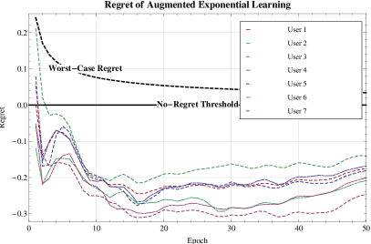
(a) No regret under augmented exponential learning.

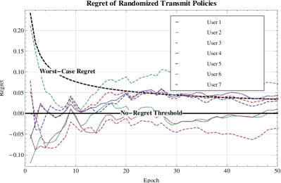
(b) Positive regret under randomized power allocation.

Figure 1: The long-term regret induced by augmented exponential learning and a random sampling transmit policy (Figs 1(a) and 1(b) respectively) for different users (see text for details). In tune with Theorem 1, AXL quickly falls below the no-regret threshold whereas the randomized policy (29) leads to positive regret for several users (in both figures the dashed “worst-case regret” curve represents the regret guarantee (22) of the AXL algorithm).

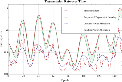
(a) Performance of AXL with average user velocity $v=5~{}\mathrm{km/s}$.

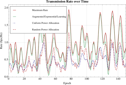
(b) Performance of AXL with average user velocity $v=15~{}\mathrm{km/s}$.

Figure 2: Data rates achieved by AXL in a changing environment with different fading velocities: the dynamic transmit policy induced by the AXL algorithm allows users to track their maximum achievable transmission rate remarkably well even under rapidly changing channel conditions.

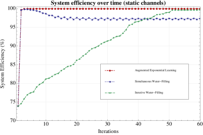
(a) Learning with perfect CSI.

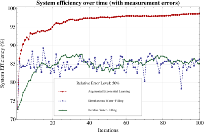
(b) Learning with an average relative error level of 50%.

Figure 3: Convergence and robustness of AXL with imperfect CSI in a MIMO MAC system with $10$ PUs and $25$ SUs: in contrast to water-filling methods, AXL attains the channel’s sum capacity even in the presence of very high measurement errors.

VI Conclusions

In this paper, we introduced an adaptive transmit policy for MIMO-OFDM cognitive radio systems that evolve dynamically over time as a function of changing user and environmental conditions. Drawing on the method of matrix exponential learning [22] and online mirror descent [18, 23], we derived an augmented exponential learning (AXL) scheme which leads to no regret: for every SU, the proposed transmit policy performs asymptotically as well as the best fixed transmit profile over the entire transmission horizon, and irrespective of how the system evolves over time. In fact, this learning scheme is closely aligned to the direction of change of the users’ data rate function, so the system’s SUs are able to track their individual optimum transmit profile even under rapidly changing conditions. Importantly, the implementation of the proposed algorithm requires only local CSI; moreover, the algorithm retaints its no-regret properties even in the case of imperfect CSI (with arbitrarily large measurement errors) and significantly outperforms classical water-filling algorithms (where the use of perfect CSI is critical).

To a large extent, our dynamic transmit policy owes its no-regret properties to an associated entropy function (for instance, the von Neumann quantum entropy for the problem’s signal covariance component). As a result, by choosing a proper entropy-like kernel (e.g. as in [36]), we can examine significantly more general situations, including for example pricing and/or energy-awareness constraints.

Finally, we should mention here that when the environment undergoes rapid changes, there are other regret notions which are more suited to adaptability (such as the adaptive regret measure of [28]). Studying the performance of augmented exponential learning with respect to different regret valuations lies beyond the scope of the current paper, but we intend to explore this direction in future work.

[Technical Proofs]

Our proof approach relies on a technique introduced by Sorin [39] and recently extended by J. Kwon and one of the authors to more general online mirror descent methods [35]. First, we will establish the no-regret property of augmented exponential learning in continuous time; subsequently, we derive the corresponding discrete-time result by estimating the difference between the continuous- and discrete-time processes.

-A Online Power Allocation: the Case $P_{k}\geq P$.

To begin with, note that the exponential mapping of (XL-PA) may be characterized as the solution of the convex program:

maximize $$\left\langle\mathbf{y}\middle|\mathbf{q}\right\rangle-h(\mathbf{q}),$$ (31)

subject to $$q_{k}\geq 0,\;\sum_{k}q_{k}=1,$$

where $\left\langle\mathbf{y}\middle|\mathbf{q}\right\rangle$ denotes the bilinear pairing $\left\langle\mathbf{y}\middle|\mathbf{q}\right\rangle=\sum_{k}q_{k}y_{k}$ and $h(\mathbf{q})=\sum_{k}q_{k}\log q_{k}$ denotes the Gibbs–Shannon entropy on the simplex $\Delta\equiv\Delta(\mathcal{K})$ spanned by $\mathcal{K}$. More precisely, we have the following classical result [40, Chapter 25]:

Lemma 1.

For every $\mathbf{y}\in\mathbb{R}^{K}$, the problem (31) admits the unique solution $G(\mathbf{y})$ with $G_{k}(\mathbf{y})=e^{y_{k}}\big{/}\sum_{\ell}e^{y_{\ell}}$.

Consider now the following continuous-time variant of (XL-PA) for $t\geq 0$:

$$\dot{y}_{k} =\frac{\partial\Phi}{\partial q_{k}},$$ (32)

$$\mathbf{q}(t) =G\left(\gamma(t)\mathbf{y}(t)\right),$$

where $\gamma(t)=\min\{\eta,\eta t^{-1/2}\}$; moreover, define the cumulative continuous-time regret with respect to some fixed $\mathbf{q}_{0}\in\Delta$ as

$$\operatorname{Reg}_{T}^{c}(\mathbf{q}_{0})=\int_{0}^{T}\big{[}\Phi(\mathbf{q}_{0};t)-\Phi(\mathbf{q}(t);t)\big{]}\>dt,$$ (33)

where $\Phi(\cdot;t)$, is a piecewise continuous stream of rate functions and the index $c$ in $\operatorname{Reg}_{T}^{c}$ indicates that we are working in continuous time. We then have:

Proposition 4.

The cumulative regret generated by the learning scheme (32) satisfies $\operatorname{Reg}_{T}^{c}(\mathbf{q}_{0})\leq\eta^{-1}\log K\cdot\sqrt{T}$ for all $\mathbf{q}_{0}\in\Delta$.

Proof:

Let $h^{\ast}(\mathbf{y})$ denote the convex conjugate of $h$, i.e. $h^{\ast}(\mathbf{y})=\max_{\mathbf{q}\in\Delta}\{\left\langle\mathbf{y}\middle|\mathbf{q}\right\rangle-h(\mathbf{q})\}=\left\langle\mathbf{y}\middle|G(\mathbf{y})\right\rangle-h(G(\mathbf{y})).$ Moreover, set $\gamma(t)=\min\{\eta t^{-1/2},\eta\}$ and let $\mathbf{q}(t)$ be defined as in (32) with $\mathbf{v}(t)=\dot{\mathbf{y}}(t)=\nabla_{\mathbf{q}(t)}\Phi(\mathbf{q}(t);t)$. By Lemma 1, we will have $h^{\ast}(\gamma\mathbf{y})=\log\sum_{\ell}e^{\gamma y_{\ell}}$ and hence:

$$\frac{d}{dt}h^{\ast}(\gamma\mathbf{y})=\sum_{k\in\mathcal{K}}\left.\frac{\partial h^{\ast}}{\partial y_{k}}\right|_{\gamma\mathbf{y}}\left(\dot{\gamma}y_{k}+\gamma\dot{y}_{k}\right)=\dot{\gamma}\left\langle\mathbf{y}\middle|\mathbf{q}\right\rangle+\gamma\left\langle\mathbf{v}\middle|\mathbf{q}\right\rangle,$$ (34)

where we used (32) and the fact that $\nabla_{\mathbf{y}}h^{\ast}(\mathbf{y})=G(\mathbf{y})$. By isolating $\left\langle\mathbf{v}\middle|\mathbf{q}\right\rangle$ and integrating by parts, we then get:

$$\int_{0}^{T}\left\langle\mathbf{v}\middle|\mathbf{q}\right\rangle\>dt =\frac{h^{\ast}(\gamma(T)\mathbf{y}(T))}{\gamma(T)}-\frac{h^{\ast}(\gamma(0)\mathbf{y}(0))}{\gamma(0)}+\int_{0}^{T}\frac{\dot{\gamma}}{\gamma^{2}}h^{\ast}(\gamma\mathbf{y})\>dt-\int_{0}^{T}\frac{\dot{\gamma}}{\gamma}\left\langle\mathbf{y}\middle|\mathbf{q}\right\rangle\>dt$$

$$=\frac{h^{\ast}(\gamma(T)\mathbf{y}(T))}{\gamma(T)}-\frac{h^{\ast}(0)}{\gamma(0)}-\int_{0}^{T}\frac{\dot{\gamma}}{\gamma^{2}}h(G(\gamma\mathbf{y}))\>dt,$$ (35)

where the last step follows from the fact that $\mathbf{q}=G(\gamma\mathbf{y})$ and the defining relation $h^{\ast}(\gamma\mathbf{y})=\left\langle\gamma\mathbf{y}\middle|G(\gamma\mathbf{y})\right\rangle-h(G(\gamma\mathbf{y}))$. Then, given that the minimum of $h$ over $\Delta$ is $-\log K$, we also have $h^{\ast}(0)=-h_{\min}=\log K$; thus, with $\dot{\gamma}\leq 0$, (-A) becomes:

$$\int_{0}^{T}\left\langle\mathbf{v}\middle|\mathbf{q}\right\rangle\>dt \geq\frac{h^{\ast}(\gamma(T)\mathbf{y}(T))}{\gamma(T)}-\frac{h^{\ast}(0)}{\gamma(0)}+h^{\ast}(0)\int_{0}^{T}\frac{\dot{\gamma}}{\gamma^{2}}\>dt$$

$$\geq\frac{\left\langle\gamma(T)\mathbf{y}(T)\middle|\mathbf{q}_{0}\right\rangle-h(\mathbf{q}_{0})}{\gamma(T)}-\frac{\log K}{\gamma(T)}$$

$$\geq\left\langle\mathbf{y}(T)\middle|\mathbf{q}_{0}\right\rangle-\frac{\log K}{\eta}\sqrt{T},$$ (36)

where we used the fact that $h^{\ast}(\gamma\mathbf{y})\geq\left\langle\gamma\mathbf{y}\middle|\mathbf{q}_{0}\right\rangle-h(\mathbf{q}_{0})$ for all $\mathbf{q}_{0}\in\Delta$ in the second line and that $h\leq 0$ in the last step. With $\Phi$ concave over $\Delta$, we will also have $\Phi(\mathbf{q}_{0};t)-\Phi(\mathbf{q}(t);t)\leq\left\langle\nabla_{\mathbf{q}(t)}\Phi\middle|\mathbf{q}_{0}-\mathbf{q}(t)\right\rangle=\left\langle\mathbf{v}(t)\middle|\mathbf{q}_{0}-\mathbf{q}(t)\right\rangle$; hence, by (-A), we get:

$$\operatorname{Reg}_{T}^{c}(\mathbf{q}_{0})\leq\int_{0}^{T}\left\langle\mathbf{v}\middle|\mathbf{q}_{0}-\mathbf{q}\right\rangle\>dt\leq\frac{\log K}{\eta}\sqrt{T},$$ (37)

and our proof is complete. ∎

-B Online Power Allocation: The General Case.

If $P_{k}<P$ for some $k$, we still obtain a no-regret power allocation policy if we use the modified entropy function $h(p)=\sum_{k}\left(p_{k}\log p_{k}+(P_{k}-p_{k})\log(P_{k}-p_{k})\right),$ and define the modified Gibbs map:

$$G_{0}(\mathbf{y})=\operatorname*{\arg\max}_{\mathbf{p}\in\mathcal{X}_{0}}\big{\{}\left\langle\mathbf{y}\middle|\mathbf{p}\right\rangle-h_{0}(\mathbf{p})\big{\}}.$$ (38)

Specifically, consider the following modified version of (32):

$$\dot{y}_{k} =\frac{\partial\Phi}{\partial p_{k}},$$ (39)

$$\mathbf{p}(t) =G_{0}\left(\gamma(t)\mathbf{y}(t)\right),$$

where $\Phi(\cdot;t)$ is a continuous stream of rate functions of the form (5) and $\gamma=\min\{\eta,\eta t^{-1/2}\}$. We then have:

Proposition 5.

The learning scheme (39) leads to no regret in continuous time: $\operatorname{Reg}_{T}^{c}(\mathbf{p}_{0})\leq\operatorname{\mathcal{O}}(\sqrt{T})\quad\text{for all $\mathbf{p}_{0}\in\mathcal{X}_{0}$.}$

Proof:

As in the proof of Proposition 4, let $h_{0}^{\ast}(\mathbf{y})=\max_{\mathbf{p}\in\mathcal{X}_{0}}\{\left\langle\mathbf{y}\middle|\mathbf{p}\right\rangle-h_{0}(\mathbf{p})\}=\left\langle\mathbf{y}\middle|G_{0}(\mathbf{y})\right\rangle-h_{0}(G_{0}(\mathbf{y}))$ be the convex conjugate of $h_{0}(\mathbf{p})$. Since the derivative of $h_{0}$ blows up to infinity at the boundary of $\mathcal{X}_{0}$, the unique solution to the maximization problem defining $G_{0}$ lies at the interior of $\mathcal{X}_{0}$. The Karush–Kuhn–Tucker (KKT) conditions thus give $y_{k}-\frac{\partial h_{0}}{\partial p_{k}}=\lambda,$ where $\lambda$ is the Lagrange multiplier for the equality constraint $\sum_{\ell}p_{\ell}=P$. We will then also have $\frac{\partial h_{0}^{\ast}}{\partial y_{k}}=G_{0,k}(\mathbf{y})+\sum\nolimits_{\ell=1}^{K}y_{\ell}\frac{\partial}{\partial y_{k}}G_{0,\ell}(\mathbf{y})-\sum\nolimits_{\ell=1}^{K}\frac{\partial h_{0}}{\partial p_{\ell}}\frac{\partial}{\partial y_{k}}G_{0,\ell}(\mathbf{y})=G_{0,k}(\mathbf{y}),$ where, in the last step, we used the fact that $\sum_{\ell=1}^{K}G_{0,\ell}(\mathbf{y})=P$ (so $\sum_{\ell=1}^{K}\partial_{y_{k}}G_{0,\ell}=0$ for all $k$). Thus, letting $\mathbf{v}(t)=\nabla_{\mathbf{p}}\Phi(\mathbf{p};t)$ so that $\mathbf{y}(t)=\int_{0}^{t}\mathbf{v}(s)\>ds$ and $\mathbf{p}(t)=G_{0}(\gamma(t)\mathbf{y}(t))$, we obtain the basic identity:

$$\frac{d}{dt}h_{0}^{\ast}(\gamma\mathbf{y})=\sum_{k\in\mathcal{K}}\left.\frac{\partial h_{0}^{\ast}}{\partial y_{k}}\right|_{\gamma\mathbf{y}}\left(\dot{\gamma}y_{k}+\gamma\dot{y}_{k}\right)=\dot{\gamma}\left\langle\mathbf{y}\middle|\mathbf{p}\right\rangle+\gamma\left\langle\mathbf{v}\middle|\mathbf{p}\right\rangle,$$ (40)

and the rest of the proof follows as in the case of Prop. 4. ∎

-C Online Signal Covariance Optimization

For the MIMO component (OCOV) of (ORM) we will consider the continuous-time scheme:

$$\dot{\mathbf{Y}}_{k} =\frac{\partial\Phi}{\partial\mathbf{Q}_{k}^{\ast}},$$ (41)

$$\mathbf{Q}_{k} =\frac{\exp(\gamma\mathbf{Y}_{k})}{\operatorname{tr}\left[\exp\left(\gamma\mathbf{Y}_{k}\right)\right]}.$$

where, as before, $\gamma=\min\{\eta,\eta t^{-1/2}\}$. Then, with the user’s regret defined as in (33), we get:

Proposition 6.

The cumulative regret generated by the continuous-time learning scheme (41) satisfies $\operatorname{Reg}_{T}^{c}(\mathbf{Q}_{0})\leq\eta^{-1}\sqrt{T}\sum_{k=1}^{K}\log m_{k}\text{ for all $\textstyle\mathbf{Q}_{0}\in\mathcal{X}_{+}\equiv\prod_{k=1}^{K}\mathcal{D}_{k}$.}$

To prove Proposition 6, we first show that the matrix exponential of (21) solves the semidefinite problem:

maximize $$\operatorname{tr}\big{[}\mathbf{Y}\mathbf{Q}\big{]}-h_{+}(\mathbf{Q}),$$ (42)

subject to $$\mathbf{Q}\succcurlyeq 0,\;\operatorname{tr}(\mathbf{Q})=1,$$

where $\mathbf{Y}$ is a Hermitian matrix and $h_{+}(\mathbf{Q})=\operatorname{tr}\big{[}\mathbf{Q}\log\mathbf{Q}\big{]}$ is the von Neumann entropy. Indeed:

Lemma 2.

For every Hermitian matrix $\mathbf{Y}\in\mathbb{C}^{m\times m}$, the problem (31) admits the unique solution $\mathbf{Q}_{\mathbf{Y}}=\exp(\mathbf{Y})\big{/}\operatorname{tr}\big{[}\exp(\mathbf{Y})\big{]}$. Accordingly, the convex conjugate $h_{+}^{\ast}$ of $h_{+}$ is:

$$h_{+}^{\ast}(\mathbf{Y})=\max\nolimits_{\mathbf{Q}\in\mathcal{D}}\left\{\operatorname{tr}\big{[}\mathbf{Y}\mathbf{Q}\big{]}-h_{+}(\mathbf{Q})\right\}=\log\operatorname{tr}\big{[}\exp(\mathbf{Y})\big{]}.$$ (43)

Proof:

To begin with, let $A(\mathbf{Y},\mathbf{Q})=\operatorname{tr}\big{[}\mathbf{Y}\mathbf{Q}]-h_{+}(\mathbf{Q})$ denote the objective of the problem (42), and let $Z=\{\mathbf{A}\in\mathbb{C}^{m\times m}:\mathbf{A}^{{\dagger}}=\mathbf{A},\operatorname{tr}(\mathbf{A})=0\}$ be the space of tangent directions to $\mathcal{D}$. Then, if $\{q_{j},\mathbf{u}_{j}\}_{j=1}^{m}$ is an eigen-decomposition of $\mathbf{Q}+t\mathbf{Z}$ for $\mathbf{Q}\in\mathcal{D}^{\circ}$ and $\mathbf{Z}\in Z$, we will have $A(\mathbf{Y},\mathbf{Q}+t\mathbf{Z})=\operatorname{tr}[\mathbf{Y}\mathbf{Q}]+\operatorname{tr}[\mathbf{Y}\mathbf{Z}]\,t-\sum\nolimits_{j}q_{j}\log q_{j}.$ Hence, the directional derivative of $A(\mathbf{Y},\mathbf{Q})$ along $\mathbf{Z}$ at $\mathbf{Q}$ is $\nabla_{\mathbf{Z}}A(\mathbf{Y},\mathbf{Q})=\left.\frac{d}{dt}\right|_{t=0}A(\mathbf{Y},\mathbf{Q}+t\mathbf{Z})=\operatorname{tr}[\mathbf{Y}\mathbf{Z}]-\sum\nolimits_{k=1}^{K}\dot{q}_{k}\log q_{k}$ where we have used the fact that $\sum\nolimits_{j}\dot{q}_{j}=0$ (recall that $\sum\nolimits_{j}q_{j}=\operatorname{tr}(\mathbf{Q}+t\mathbf{Z})=1$ for all $t$ such that $\mathbf{Q}+t\mathbf{Z}\in\mathcal{D}^{\circ}$). However, differentiating the defining relation $(\mathbf{Q}+t\mathbf{Z})\mathbf{u}_{j}=q_{j}\mathbf{u}_{j}$ with respect to $t$ gives $\mathbf{Z}\mathbf{u}_{j}+(\mathbf{Q}+t\mathbf{Z})\dot{\mathbf{u}}_{j}=\dot{q}_{j}\mathbf{u}_{j}+q_{j}\dot{\mathbf{u}}_{j},$ so, after multiplying from the left by $\mathbf{u}_{j}^{{\dagger}}$, we get $\dot{q}_{j}=\mathbf{u}_{j}^{{\dagger}}\mathbf{Z}\mathbf{u}_{j}+\mathbf{u}_{j}^{{\dagger}}(\mathbf{Q}+t\mathbf{Z})\dot{\mathbf{u}}_{j}-q_{j}\mathbf{u}_{j}^{{\dagger}}\dot{\mathbf{u}}_{j}=\mathbf{u}_{j}^{{\dagger}}\mathbf{Z}\mathbf{u}_{j}.$ Summing over $j$ gives $\sum\nolimits_{j}\dot{q}_{j}\log q_{j}=\sum\nolimits_{j}\mathbf{u}_{j}^{{\dagger}}\mathbf{Z}\mathbf{u}_{j}\log q_{j}=\operatorname{tr}[\mathbf{Z}\log\mathbf{Q}]$; then, by substituting in the previous expression for $\nabla_{\mathbf{Z}}A(\mathbf{Y},\mathbf{Q})$, we finally obtain $\nabla_{\mathbf{Z}}A(\mathbf{Y},\mathbf{Q})=\operatorname{tr}[\mathbf{Z}(\mathbf{Y}-\log\mathbf{Q})].$

By standard convex-analytic arguments, it follows that (42) admits a unique solution $\mathbf{Q}_{\mathbf{Y}}$ at the interior $\mathcal{D}^{\circ}$ of $\mathcal{D}$ [40, Chapter 26]. Accordingly, by the KKT conditions for (42), we have $\nabla_{\mathbf{Z}}A(\mathbf{Y},\mathbf{Q}_{\mathbf{Y}})=0$ for all tangent directions $\mathbf{Z}$ to $\mathcal{D}^{\circ}$ at $\mathbf{Q}_{\mathbf{Y}}$, i.e. $\operatorname{tr}[\mathbf{Z}(\mathbf{Y}-\log\mathbf{Q}_{\mathbf{Y}})]=0$ for all Hermitian $\mathbf{Z}\in\mathbb{C}^{m\times m}$ such that $\operatorname{tr}(\mathbf{Z})=0$. From this last condition, we immediately get $\mathbf{Y}-\log\mathbf{Q}_{\mathbf{Y}}\propto\mathbf{I}$, and with $\operatorname{tr}(\mathbf{Q}_{\mathbf{Y}})=1$, we obtain $\mathbf{Q}_{\mathbf{Y}}=\exp(\mathbf{Y})/\operatorname{tr}[\exp(\mathbf{Y})]$; the expression for $h_{+}^{\ast}(\mathbf{Y})$ then follows by substituting $\mathbf{Q}_{\mathbf{Y}}$ in the definition of $A(\mathbf{Y},\mathbf{Q})$. ∎

Armed with this characterization, we now get:

Proof:

Let $h_{k}(\mathbf{Q}_{k})=\operatorname{tr}(\mathbf{Q}_{k}\log\mathbf{Q}_{k})$, $\mathbf{Q}_{k}\in\mathcal{D}_{k}$, so $h_{k}^{\ast}(\mathbf{Y}_{k})=\log\operatorname{tr}[\exp(\mathbf{Y}_{k})]$ by Lemma 2; moreover, let $\mathbf{Q}=\operatorname{diag}(\mathbf{Q}_{1},\dotsc,\mathbf{Q}_{K})$ and set $h_{+}(\mathbf{Q})=\sum_{k}h_{k}(\mathbf{Q}_{k})=\operatorname{tr}\big{[}\mathbf{Q}\log\mathbf{Q}\big{]}$ for $\mathbf{Q}\in\mathcal{X}_{+}\equiv\prod_{k}\mathcal{D}_{k}$. Then, if $\mathbf{Y}=\operatorname{diag}(\mathbf{Y}_{1},\dotsc,\mathbf{Y}_{K})$ with $\mathbf{Y}_{k}$ Hermitian, we will have $h_{+}^{\ast}(\mathbf{Y})=\max_{\mathbf{Q}\in\mathcal{X}_{+}}\left\{\operatorname{tr}\big{[}\mathbf{Y}\mathbf{Q}\big{]}-h(\mathbf{Q})\right\}=\sum\nolimits_{k}h_{k}^{\ast}(\mathbf{Y}_{k})=\sum\nolimits_{k}\log\operatorname{tr}\big{[}\exp(\mathbf{Y}_{k})\big{]}.$ Accordingly, if we let $\mathbf{V}_{k}(t)=\partial_{\mathbf{Q}_{k}^{\ast}}\Phi(\mathbf{Q};t)$, we get:

$$\frac{d}{dt}h_{+}^{\ast}(\gamma\mathbf{Y}) =\sum\nolimits_{k=1}^{K}\operatorname{tr}\big{[}\exp(\gamma\mathbf{Y}_{k})\big{]}^{-1}\frac{d}{dt}\operatorname{tr}\big{[}\exp(\gamma\mathbf{Y}_{k})\big{]}$$

$$=\sum\nolimits_{k=1}^{K}\operatorname{tr}\big{[}\exp(\gamma\mathbf{Y}_{k})\big{]}^{-1}\operatorname{tr}\big{[}\big{(}\dot{\gamma}\mathbf{Y}_{k}+\gamma\dot{\mathbf{Y}}_{k}\big{)}\exp(\mathbf{Y}_{k})\big{]}$$

$$=\dot{\gamma}\operatorname{tr}\big{[}\mathbf{Y}\mathbf{Q}\big{]}+\gamma\operatorname{tr}\big{[}\mathbf{V}\mathbf{Q}\big{]}$$ (44)

where we set $\mathbf{V}=\operatorname{diag}(\mathbf{V}_{1},\dotsc,\mathbf{V}_{K})$. Following the same steps as in the proof of Proposition 4, we then obtain:

$$\int_{0}^{T}\operatorname{tr}\big{[}\mathbf{V}\mathbf{Q}\big{]}\>dt=\frac{h_{+}^{\ast}(\gamma(T)\mathbf{Y}(T))}{\gamma(T)}-\frac{h_{+}^{\ast}(0)}{\gamma(0)}-\int_{0}^{T}\frac{\dot{\gamma}}{\gamma^{2}}h_{+}(\mathbf{Q})\>dt,$$ (45)

The minimum of $h_{+}$ over $\mathcal{X}_{+}=\prod_{k}\mathcal{D}_{k}$ is just $-\sum_{k}\log m_{k}$, so we also have $h^{\ast}(0)=-\min_{\mathbf{Q}\in\mathcal{X}_{+}}h_{+}(\mathbf{Q})=\sum_{k}\log m_{k}$; then, with $\dot{\gamma}\leq 0$, (45) becomes:

$$\int_{0}^{T}\operatorname{tr}\big{[}\mathbf{V}\mathbf{Q}\big{]}\>dt \geq\frac{h_{+}^{\ast}(\gamma(T)\mathbf{Y}(T))}{\gamma(T)}-\frac{h^{\ast}(0)}{\gamma(0)}+h_{+}^{\ast}(0)\int_{0}^{T}\frac{\dot{\gamma}}{\gamma^{2}}\>dt$$

$$\geq\frac{\operatorname{tr}\big{[}\gamma(T)\mathbf{Y}(T)\mathbf{Q}_{0}\big{]}-h_{+}(\mathbf{Q}_{0})}{\gamma(T)}-\frac{\sum_{k=1}^{K}\log m_{k}}{\gamma(T)}$$

$$\geq\operatorname{tr}\big{[}\mathbf{Y}(T)\mathbf{Q}_{0}\big{]}-\frac{\sum_{k=1}^{K}\log m_{k}}{\eta}\sqrt{T},$$ (46)

where we used the fact that $h_{+}^{\ast}(\gamma\mathbf{Y})\geq\operatorname{tr}\big{[}\gamma\mathbf{Y}\mathbf{Q}_{0}\big{]}-h_{+}(\mathbf{Q}_{0})$ for all $\mathbf{Q}_{0}\in\mathcal{X}_{+}$ in the second line and the fact that $h_{+}\leq 0$ in the last step. Since $\Phi$ is concave in $\mathbf{Q}$ and $\mathbf{V}=\nabla_{\mathbf{Q}^{\ast}}\Phi$, the rest of the proof follows in the same way as that of Proposition 4. ∎

-D The Full MIMO–OFDM Problem

Our final step in this continuous-time setting will be to establish the no-regret properties of the following continuous-time variant of the AXL algorithm for $P_{k}\geq P$:

$$\dot{y}_{k} =\frac{\partial\Phi}{\partial q_{k}}, \dot{\mathbf{Y}}_{k} =\frac{\partial\Phi}{\partial\mathbf{Q}_{k}^{\ast}},$$ (47)

$$q_{k} =\frac{\exp(\gamma y_{k})}{\sum_{\ell=1}^{K}\exp(\gamma y_{\ell})}, \mathbf{Q}_{k} =\frac{\exp(\gamma\mathbf{Y}_{k})}{\operatorname{tr}\left[\exp(\gamma\mathbf{Y}_{k})\right]},$$

with $\gamma=\min\{\eta,\eta t^{-1/2}\}$ as usual. Without further ado, we have:

Proposition 7.

If $P_{k}\geq P$ for all $k\in\mathcal{K}$, then, for all $\mathbf{P}_{0}\in\mathcal{X}$, the cumulative regret generated by (47) will satisfy $\operatorname{Reg}_{T}^{c}(\mathbf{P}_{0})\leq\eta^{-1}\sqrt{T}\left(\log K+\sum_{k=1}^{K}\log m_{k}\right).$

Proof:

Recall that any $\mathbf{P}\in\mathcal{X}$ may be decomposed as $\mathbf{P}=\operatorname{diag}(p_{1}\mathbf{Q}_{1},\dotsc,p_{K}\mathbf{Q}_{K})$ with $\mathbf{p}=(p_{1},\dotsc,p_{K})\in\mathcal{X}_{0}$ and $\mathbf{Q}=\operatorname{diag}(\mathbf{Q}_{1},\dotsc,\mathbf{Q}_{K})\in\mathcal{X}_{+}\equiv\prod_{k}\mathcal{D}_{k}$. Then, using the normalized power allocation vector $\mathbf{q}=\mathbf{p}/P\in\Delta$ for convenience, let $H(\mathbf{q},\mathbf{Q})=h(\mathbf{q})+h_{+}(\mathbf{Q})=\sum\nolimits_{k=1}^{K}\big{[}q_{k}\log q_{k}+\operatorname{tr}(\mathbf{Q}_{k}\log\mathbf{Q}_{k})\big{]}$ and consider the associated Legendre–Fenchel problem:

maximize $$\left\langle\mathbf{y}\middle|\mathbf{q}\right\rangle+\operatorname{tr}[\mathbf{Y}\mathbf{Q}]-H(\mathbf{q},\mathbf{Q}),$$ (48)

subject to $$\mathbf{q}\in\Delta,\;\mathbf{Q}\in\prod\nolimits_{k}\mathcal{D}_{k}.$$

Clearly, (48) may be decomposed as a sum of (31) and (42), so each component of the solution of (48) is given by Lemmas 1 and 2 respectively; likewise, the convex conjugate of $H$ will be $H^{\ast}(\mathbf{y},\mathbf{Y})=h^{\ast}(\mathbf{y})+h_{+}^{\ast}(\mathbf{Y})$, with $h^{\ast}$ and $h_{+}^{\ast}$ defined as before. Our claim is then obtained by following the same steps as in the proofs of Propositions 4 and 6. ∎

-E The Descent to Discrete Time

In this appendix, we to derive the no-regret properties of the discrete-time policies (XL-PA), (XL-COV) and of the AXL algorithm (Propositions 1, 3 and Theorem 1 respectively) by means of a comparison technique introduced by Sorin [39] and developed further by J. Kwon and one of the authors [35]. Specifically, we have:

Lemma 3.

Let $\mathcal{C}$ be a compact convex set in $\mathbb{R}^{N}$, let $\mathbf{v}(t)$ be a sequence of payoff vectors in $\mathbb{R}^{N}$ with $\|\mathbf{v}(t)\|\leq V$ in the uniform norm of $\mathbb{R}^{N}$ ($t=1,2\dotsc$), and consider the sequence of play $\mathbf{x}(t+1)=Q\left(\eta t^{-1/2}\sum\nolimits_{s=1}^{t}\mathbf{v}(s)\right)$ where $Q\colon\mathbb{R}^{N}\to\mathcal{C}$ is $C$-Lipschitz with respect to the $L^{1}$ norm on $\mathcal{C}$. Moreover, letting $\mathbf{v}^{c}(t)=\mathbf{v}(\left\lceil t\right\rceil)$ be a piecewise constant interpolation of $\mathbf{v}(t)$ for $t\in[1,+\infty)$, consider the continuous-time process $\mathbf{x}^{c}(t)=Q\left(\gamma(t)\int_{0}^{t}\mathbf{v}^{c}(s)\>ds\right)$ with $\gamma(t)=\min\{\eta t^{-1/2},\eta\}$, and assume that it guarantees the regret bound:

$$\int_{0}^{T}\left\langle\mathbf{v}^{c}(t)\middle|\mathbf{x}_{0}-\mathbf{x}^{c}(t)\right\rangle\>dt\leq R(T)\sqrt{T}\quad\text{for all $\mathbf{x}_{0}\in\mathcal{X}_{+}$.}$$ (49)

Then, for all $\mathbf{x}_{0}\in\mathcal{A}$, the discrete-time sequence $\mathbf{x}(t)$ guarantees

$$\sum\nolimits_{t=1}^{T}\left\langle\mathbf{v}(t)\middle|\mathbf{x}_{0}-\mathbf{x}(t)\right\rangle\leq\sqrt{T}\left(R(T)+4CV^{2}\eta\right).$$ (50)

Proof:

By assumption, if we set $\mathbf{y}(t)=\int_{0}^{t}\mathbf{v}^{c}(s)\>ds$, we have $\mathbf{x}^{c}(t)=Q(\gamma(t)\mathbf{y}(t))=\mathbf{x}(t+1)$ whenever $t$ is a positive integer. Hence, for every integer $T\geq 1$, we have $\int_{0}^{T}\left\langle\mathbf{v}^{c}(t)\middle|\mathbf{x}^{c}(t)\right\rangle\>dt-\sum_{t=1}^{T}\left\langle\mathbf{v}(t)\middle|\mathbf{x}(t)\right\rangle=\int_{0}^{T}\left\langle\mathbf{v}^{c}(t)\middle|\mathbf{x}^{c}(t)\right\rangle\>dt-\int_{0}^{T}\left\langle\mathbf{v}(\left\lceil t\right\rceil)\middle|\mathbf{x}(\left\lceil t\right\rceil)\right\rangle\>dt=\int_{0}^{T}\left\langle\mathbf{v}^{c}(t)\middle|\mathbf{x}^{c}(t)-\mathbf{x}^{c}(\left\lfloor t\right\rfloor)\right\rangle\>dt$ where we used the fact that $\mathbf{x}^{c}(\left\lfloor t\right\rfloor)=\mathbf{x}(\left\lceil t\right\rceil)$ in the second step. On the other hand, Hölder’s inequality gives $\left|\left\langle\mathbf{v}^{c}(t)\middle|\mathbf{x}^{c}(t)-\mathbf{x}^{c}(\left\lfloor t\right\rfloor)\right\rangle\right|\leq\|\mathbf{v}^{c}(t)\|_{\infty}\cdot\|\mathbf{x}^{c}(t)-\mathbf{x}^{c}(\left\lfloor t\right\rfloor)\|_{1}\leq V\,\|\mathbf{x}^{c}(t)-\mathbf{x}^{c}(\left\lfloor t\right\rfloor)\|_{1}\leq V\,\|Q(\gamma(t)\mathbf{y}(t))-Q(\gamma(\left\lfloor t\right\rfloor)\mathbf{y}(\left\lfloor t\right\rfloor))\|_{1}\leq CV\,\|\gamma(t)\mathbf{y}(t)-\gamma(\left\lfloor t\right\rfloor)\mathbf{y}(\left\lfloor t\right\rfloor)\|_{\infty}.$ The last term may then be rewritten as:

$$\|\gamma(t)\mathbf{y}(t)-\gamma(\left\lfloor t\right\rfloor)\mathbf{y}(\left\lfloor t\right\rfloor)\|_{\infty} =\left\|\int_{\left\lfloor t\right\rfloor}^{t}\frac{d}{ds}\left(\gamma(s)\mathbf{y}(s)\right)\>ds\right\|_{1}$$ (51)

$$\leq\int_{\left\lfloor t\right\rfloor}^{t}\left\|\gamma(s)\mathbf{v}^{c}(s)+\dot{\gamma}(s)\int_{0}^{s}\mathbf{v}^{c}(w)\>dw\,\right\|_{\infty}\>ds\leq V\int_{\left\lfloor t\right\rfloor}^{t}\left(\gamma(s)-s\dot{\gamma}(s)\right)\>ds.$$ (52)

Recalling that $\gamma(t)=\min\{\eta,\eta t^{-1/2}\}$, this last integral is equal to $\eta t$ if $t\in[0,1]$ and $3\eta\big{(}t^{1/2}-\left\lfloor t\right\rfloor^{1/2}\big{)}$ otherwise. Thus, combining the above inequalities, we obtain:

$$\int_{0}^{T}\!\!\!\left\langle\mathbf{v}^{c}(t)\middle|\mathbf{x}^{c}(t)-\mathbf{x}^{c}(\left\lfloor t\right\rfloor)\right\rangle\>dt \leq CV^{2}\!\!\!\int_{0}^{T}\!\!\!\int_{\left\lfloor t\right\rfloor}^{t}\left(\gamma(s)-s\dot{\gamma}(s)\right)\>ds\>dt$$ (53)

$$\leq CV^{2}\eta\left(\frac{1}{2}+3\sum_{k=1}^{T-1}\int_{k}^{k+1}\frac{t-k}{\sqrt{t}+\sqrt{k}}\>dt\right)\leq 4CV^{2}\eta\sqrt{T}.$$ (54)

Hence, by the definition of $\mathbf{v}^{c}(t)$, we finally obtain

$$\sum\nolimits_{t=1}^{T}\left\langle\mathbf{v}(t)\middle|\mathbf{x}_{0}-\mathbf{x}(t)\right\rangle=\int_{0}^{T}\left\langle\mathbf{v}^{c}(t)\middle|\mathbf{x}_{0}-\mathbf{x}^{c}(t)\right\rangle\>dt+\int_{0}^{T}\left\langle\mathbf{v}^{c}(t)\middle|\mathbf{x}^{c}(t)-\mathbf{x}^{c}(\left\lfloor t\right\rfloor)\right\rangle\>dt\leq R(T)\sqrt{T}+4CV^{2}\eta\sqrt{T},$$

which completes our proof. ∎

With this comparison at hand, the analysis of the previous sections yields:

Proof:

Note first that $v_{k}=\frac{\partial\Phi}{\partial q_{k}}=P\operatorname{tr}\big{[}\mathbf{M}_{k}\mathbf{Q}_{k}\big{]}$, so the payoff vectors $\mathbf{v}$ of (16) are bounded in the uniform norm of $\mathbb{R}^{K}$ by $PM$ – cf. (12). Given that the Lipschitz constant of the exponential mapping $G(y)$ of (1) is $C=1$ [18], the proposition follows by combining the continuous-time bound of Proposition 4 with Lemma 3. ∎

Proof:

Note first that the modified Gibbs map of (38) simply represents the power allocation policy of (XL-PA^′): indeed, by the KKT conditions for the maximization problem defining $G_{0}$, we will have:

$$\frac{p_{k}}{P_{k}-p_{k}}=e^{\lambda-y_{k}}\implies p_{k}=P_{k}\frac{e^{y_{k}}}{e^{\lambda}+e^{y_{k}}},$$ (55)

so, given that the power vector $\mathbf{p}$ satisfies the total power constraint (7a), the Lagrange multiplier $\lambda$ must satisfy the condition $P=\sum_{k}p_{k}=\sum_{k}P_{k}(1+e^{\lambda-y_{k}})^{-1}$. Comparing this last equation with (18), we conclude that $p_{k}$ will be given by the power update step of (XL-PA^′) with $\mathbf{y}$ replaced by $\gamma\mathbf{y}$, so our claim follows by combining Proposition 5 with Lemma 3. ∎

Proof:

The matrix payoffs $\mathbf{V}_{k}=\frac{\partial\Phi}{\partial\mathbf{Q}_{k}^{\ast}}=p_{k}\mathbf{M}_{k}$ satify $\|\mathbf{V}_{k}\|\leq PM$ by (12). Moreover, the von Neumann entropy $h_{+}$ is $1$-strongly convex with respect to the $L^{1}$ norm, so the matrix exponential mapping $\mathbf{Y}\mapsto\mathbf{Q}_{\mathbf{Y}}=\exp(\mathbf{Y})\big{/}\operatorname{tr}\big{[}\exp(\mathbf{Y})\big{]}$ is $1$-Lipschitz – see e.g. [23]. Our claim then follows by combining the continuous-time bound of Proposition 6 with Lemma 3. ∎

Proof:

As in the proofs of Propositions 1 and 3, the map $(\mathbf{y},\mathbf{Y})\mapsto(\mathbf{q},\mathbf{Q})\in\Delta\times\prod_{k}\mathcal{D}_{k}$ of (47) is $1$-Lipschitz and the payoffs $(\mathbf{v},\mathbf{V}_{k})$ are bounded by $PM$ in the uniform norm of $\mathbb{R}^{K}\times\prod_{k}\mathbb{C}^{m_{k}\times m_{k}}$. The theorem then follows by combining the continuous-time bound of Proposition 7 with Lemma 3. ∎

-F Learning with Imperfect CSI

Proof:

Let $\mathbf{P}(t)=\operatorname{diag}\left(\mathbf{P}_{1}(t),\dotsc,\mathbf{P}_{k}(t)\right)\in\mathcal{X}$ be the sequence of transmit profiles generated by the AXL algorithm with noisy observations $\hat{\mathbf{M}}=\mathbf{M}+\mathbf{\Xi}$. Then, for every $\mathbf{P}_{0}\in\mathcal{X}$, we have:

$$\operatorname{Reg}_{T}(\mathbf{P}_{0})\leq\sum\nolimits_{t=1}^{T}\operatorname{tr}\left[\nabla\Phi(\mathbf{P}(t))\cdot\big{(}\mathbf{P}_{0}-\mathbf{P}(t)\big{)}\right]=\sum\nolimits_{t=1}^{T}\operatorname{tr}\left[\hat{\mathbf{M}}(t)\cdot\big{(}\mathbf{P}_{0}-\mathbf{P}(t)\big{)}\right]-\sum\nolimits_{t=1}^{T}\operatorname{tr}\left[\mathbf{\Xi}(t)\cdot\big{(}\mathbf{P}_{0}-\mathbf{P}(t)\big{)}\right],$$ (56)

where the inequality follows from the concavity of $\Phi$. Since $\mathbf{P}(t)$ is generated by the sequence of matrix payoffs $\hat{\mathbf{M}}(t)$, the first term of this expression is simply the regret generated by $\mathbf{P}(t)$ against $\hat{\mathbf{M}}(t)$, so we have

$$\sum\nolimits_{t=1}^{T}\operatorname{tr}\left[\hat{\mathbf{M}}(t)\cdot\big{(}\mathbf{P}_{0}-\mathbf{P}(t)\big{)}\right]\leq R\sqrt{T}$$ (57)

by Theorem 1 (or, more accurately, by combining (-A) and (-C) with Lemma 3).

As for the second term, it is easy to see that the process $V(t)=\operatorname{tr}\left[\mathbf{\Xi}(t)\cdot\big{(}\mathbf{P}(t)-\mathbf{P}_{0}\big{)}\right]$ is a martingale difference: indeed, since $\mathbf{P}(t)$ is fully determined by $\hat{\mathbf{M}}(1),\dotsc,\hat{\mathbf{M}}(t-1)$, we get $\operatorname{\mathbb{E}}[V(t)|\mathcal{F}_{t-1}]=\operatorname{\mathbb{E}}\big{[}\operatorname{tr}\left[\mathbf{\Xi}(t)\cdot\big{(}\mathbf{P}(t)-\mathbf{P}_{0}\big{)}\right]|\mathcal{F}_{t-1}\big{]}=\operatorname{tr}\left[\operatorname{\mathbb{E}}\big{[}\mathbf{\Xi}(t)|\mathcal{F}_{t-1}\big{]}\cdot\big{(}\mathbf{P}(t)-\mathbf{P}_{0}\big{)}\right]=0.$ Moreover, with $\|\mathbf{\Xi}\|\leq\Sigma$, we will also have $|V(t)|\leq\|\mathbf{\Xi}(t)\|\cdot\|\mathbf{P}_{0}-\mathbf{P}(t)\|_{1}\leq\Sigma\cdot D,$ where $D=\max\{\|\mathbf{P}_{0}-\mathbf{P}\|_{1}:\mathbf{P}_{0},\mathbf{P}\in\mathcal{X}\}$ denotes the $L^{1}$-diameter of $\mathcal{X}$.

The bound (26) is thus obtained by taking the expectation of $\operatorname{Reg}_{T}(\mathbf{P}_{0})$ and using the zero-mean property of $V$. Similarly, the fact that $\mathbf{P}(t)$ generates no regret almost surely (and not only in expectation) follows by noting that $T^{-1}\sum_{t=1}^{T}V(t)\to 0$ as a consequence of the strong law of large numbers for martingale differences [41, Theorem 2.18]. Finally, for the large deviations bounds (27), (56) yields:

$$\operatorname{\mathbb{P}}\left(\frac{1}{T}\operatorname{Reg}_{T}(\mathbf{P}_{0})\geq\frac{R}{\sqrt{T}}+z\right)\leq\operatorname{\mathbb{P}}\left(\,\sum\nolimits_{t=1}^{T}|V(t)|\geq Tz\right).$$ (58)

However, with $\|\mathbf{\Xi}\|\leq\Sigma$, Azuma’s inequality [42] yields $\operatorname{\mathbb{P}}\left(\,\sum\nolimits_{t=1}^{T}V(t)\geq Tz\right)\leq\exp\left(-\frac{T^{2}z^{2}}{2\sum_{t=1}^{T}\operatorname{ess}\sup|V(t)|^{2}}\right)\leq\exp\left(-\frac{Tz^{2}}{2\Sigma^{2}D^{2}}\right),$ and our claim follows. ∎

References

- [1] K. V. Schinasi, “Spectrum management: Better knowledge needed to take advantage of technologies that may improve spectrum efficiency,” United States General Accounting Office, Tech. Rep., May 2004.
- [2] FCC Spectrum Policy Task Force, “Report of the spectrum efficiency working group,” Federal Communications Comission, Tech. Rep., November 2002.
- [3] J. Mitola III and G. Q. Maguire Jr., “Cognitive radio: making software radios more personal,” IEEE Personal Commun. Mag., vol. 6, no. 4, pp. 13–18, August 1999.
- [4] Q. Zhao and B. M. Sadler, “A survey of dynamic spectrum access,” IEEE Signal Process. Mag., vol. 24, no. 3, pp. 79–89, May 2007.
- [5] S. Haykin, “Cognitive radio: Brain-empowered wireless communications,” IEEE J. Sel. Areas Commun., vol. 23, no. 2, pp. 201–220, February 2005.
- [6] A. Goldsmith, S. A. Jafar, I. Maric, and S. Srinivasa, “Breaking spectrum gridlock with cognitive radios: An information theoretic perspective,” Proc. IEEE, vol. 97, no. 5, pp. 894–914, 2009.
- [7] G. J. Foschini and M. J. Gans, “On limits of wireless communications in a fading environment when using multiple antennas,” Wireless Personal Communications, vol. 6, pp. 311–335, 1998.
- [8] I. E. Telatar, “Capacity of multi-antenna Gaussian channels,” European Transactions on Telecommunications and Related Technologies, vol. 10, no. 6, pp. 585–596, 1999.
- [9] Y. J. A. Zhang and M.-C. A. So, “Optimal spectrum sharing in MIMO cognitive radio networks via semidefinite programming,” IEEE J. Sel. Areas Commun., vol. 29, no. 2, pp. 362–373, 2011.
- [10] G. Scutari and D. P. Palomar, “MIMO cognitive radio: A game theoretical approach,” IEEE Trans. Signal Process., vol. 58, no. 2, pp. 761–780, February 2010.
- [11] J. Wang, G. Scutari, and D. P. Palomar, “Robust MIMO cognitive radio via game theory,” IEEE Trans. Signal Process., vol. 59, no. 3, pp. 1183–1201, March 2011.
- [12] N. Nie and C. Comaniciu, “Adaptive channel allocation spectrum etiquette for cognitive radio networks,” in DySPAN ’05: Proceedings of the 2005 IEEE Symposium on Dynamic Spectrum Access Networks, 2005, pp. 269–278.
- [13] A. Anandkumar, N. Michael, A. K. Tang, and A. Swami, “Distributed algorithms for learning and cognitive medium access with logarithmic regret,” IEEE J. Sel. Areas Commun., vol. 29, no. 4, pp. 731–745, April 2011.
- [14] H. Li, “Multi-agent Q-learning of channel selection in multi-user cognitive radio systems: A two by two case,” in SMC ’09: Proceedings of the 2009 International Conference on Systems, Man and Cybernetics, 2009, pp. 1893–1898.
- [15] Y. Gai, B. Krishnamachari, and R. Jain, “Learning multiuser channel allocations in cognitive radio networks: A combinatorial multi-armed bandit formulation,” in DySPAN ’10: Proceedings of the 2010 IEEE Symposium on Dynamic Spectrum Access Networks, 2010.
- [16] J. Hannan, “Approximation to Bayes risk in repeated play,” in Contributions to the Theory of Games, Volume III, ser. Annals of Mathematics Studies, M. Dresher, A. W. Tucker, and P. Wolfe, Eds. Princeton, NJ: Princeton University Press, 1957, vol. 39, pp. 97–139.
- [17] N. Cesa-Bianchi and G. Lugosi, Prediction, Learning, and Games. Cambridge University Press, 2006.
- [18] S. Shalev-Shwartz, “Online learning and online convex optimization,” Foundations and Trends in Machine Learning, vol. 4, no. 2, pp. 107–194, 2011.
- [19] V. G. Vovk, “Aggregating strategies,” in COLT ’90: Proceedings of the 3rd Workshop on Computational Learning Theory, 1990, pp. 371–383.
- [20] N. Littlestone and M. K. Warmuth, “The weighted majority algorithm,” Information and Computation, vol. 108, no. 2, pp. 212–261, 1994.
- [21] P. Auer, N. Cesa-Bianchi, and C. Gentile, “Adaptive and self-confident on-line learning algorithms,” Journal of Computer and System Sciences, vol. 64, no. 1, pp. 48–75, 2002.
- [22] P. Mertikopoulos, E. V. Belmega, and A. L. Moustakas, “Matrix exponential learning: Distributed optimization in MIMO systems,” in ISIT ’12: Proceedings of the 2012 IEEE International Symposium on Information Theory, 2012, pp. 3028–3032.
- [23] S. M. Kakade, S. Shalev-Shwartz, and A. Tewari, “Regularization techniques for learning with matrices,” The Journal of Machine Learning Research, vol. 13, pp. 1865–1890, 2012.
- [24] H. Bölcskei, D. Gesbert, and A. J. Paulraj, “On the capacity of OFDM-based spatial multiplexing systems,” IEEE Trans. Commun., vol. 50, no. 2, pp. 225–234, February 2002.
- [25] K. B. Letaief and Y. J. A. Zhang, “Dynamic multiuser resource allocation and adaptation for wireless systems,” Wireless Communications, IEEE, vol. 13, no. 4, pp. 38–47, August 2006.
- [26] J. Huang and Z. Han, Cognitive Radio Networks: Architectures, Protocols, and Standards. Auerbach Publications, CRC Press, 2010, ch. Game theory for spectrum sharing.
- [27] C. R. Stevenson, G. Chouinard, Z. Lei, W. Hu, and S. J. Shellhammer, “IEEE 802.22: The first cognitive radio wireless regional area network standard,” IEEE Commun. Mag., vol. 47, no. 1, pp. 130–138, jan 2009.
- [28] E. Hazan and C. Seshadri, “Efficient learning algorithms for changing environments,” in ICML ’09: Proceedings of the 26th International Conference on Machine Learning, 2009.
- [29] D. P. Palomar, J. M. Cioffi, and M. Lagunas, “Uniform power allocation in MIMO channels: a game-theoretic approach,” IEEE Trans. Inf. Theory, vol. 49, no. 7, p. 1707, July 2003.
- [30] H. Robbins, “Some aspects of the sequential design of experiments,” Bulletin of the American Mathematical Society, vol. 58, no. 5, pp. 527–535, 1952.
- [31] P. Mertikopoulos, E. V. Belmega, A. L. Moustakas, and S. Lasaulce, “Distributed learning policies for power allocation in multiple access channels,” IEEE J. Sel. Areas Commun., vol. 30, no. 1, pp. 96–106, January 2012.
- [32] M. Zinkevich, “Online convex programming and generalized infinitesimal gradient ascent,” in ICML ’03: Proceedings of the 20th International Conference on Machine Learning, 2003.
- [33] C. D. Cantrell, Modern mathematical methods for physicists and engineers. Cambridge, UK: Cambridge University Press, 2000.
- [34] P. Mertikopoulos and E. V. Belmega, “Adaptive spectrum management in MIMO-OFDM cognitive radio: An exponential learning approach,” in ValueTools ’13: Proceedings of the 7th International Conference on Performance Evaluation Methodologies and Tools, 2013.
- [35] J. Kwon and P. Mertikopoulos, “A continuous-time approach to online optimization,” 2014, http://arxiv.org/abs/1401.6956.
- [36] F. Alvarez, J. Bolte, and O. Brahic, “Hessian Riemannian gradient flows in convex programming,” SIAM Journal on Control and Optimization, vol. 43, no. 2, pp. 477–501, 2004.
- [37] G. Calcev, D. Chizhik, B. Göransson, S. Howard, H. Huang, A. Kogiantis, A. F. Molisch, A. L. Moustakas, D. Reed, and H. Xu, “A wideband spatial channel model for system-wide simulations,” IEEE Trans. Veh. Technol., vol. 56, no. 2, p. 389, March 2007.
- [38] G. Scutari, D. P. Palomar, and S. Barbarossa, “Simultaneous iterative water-filling for Gaussian frequency-selective interference channels,” in ISIT ’06: Proceedings of the 2006 International Symposium on Information Theory, 2006.
- [39] S. Sorin, “Exponential weight algorithm in continuous time,” Mathematical Programming, vol. 116, no. 1, pp. 513–528, 2009.
- [40] R. T. Rockafellar, Convex Analysis. Princeton, NJ: Princeton University Press, 1970.
- [41] P. Hall and C. C. Heyde, Martingale Limit Theory and Its Application, ser. Probability and Mathematical Statistics. New York: Academic Press, 1980.
- [42] K. Azuma, “Weighted sums of certain dependent random variables,” Tôhoku Mathematical Journal, vol. 19, no. 3, pp. 357–367, 1967.