Abstract

For practical construction of complex synthetic genetic networks able to perform elaborate functions it is important to have a pool of relatively simple “bio-bricks” with different functionality which can be compounded together. To complement engineering of very different existing synthetic genetic devices such as switches, oscillators or logical gates, we propose and develop here a design of synthetic multiple input distributed classifier with learning ability. Proposed classifier will be able to separate multi-input data, which are inseparable for single input classifiers. Additionally, the data classes could potentially occupy the area of any shape in the space of inputs. We study two approaches to classification, including hard and soft classification and confirm the schemes of genetic networks by analytical and numerical results.

Introduction

The current challenge facing the synthetic biology research community is the construction of relatively simple, robust and reliable genetic networks, which will mount a pool of “bio-bricks”, potentially to be connected into more complex systems. Rapid progress of experimental synthetic biology has indeed provided several synthetic genetic networks with different functionality. Since the year $2000$ with the development of two fundamental simple networks, representing the toggle switch [1] and the repressilator [2], there have been a vast number of proof-of-principle synthetic networks designed and engineered. To enumerate some of them, functionally these circuits included transcriptional or metabolic oscillators [3, 4, 5], spatially coupled and synchronised oscillators [6, 7], calculators [8], inducers of pattern formation [9], learning systems [10], optogenetic devices [11], memory circuits and logic gates [12, 13, 14, 15].

One of the much awaited kinds of synthetic gene circuits with principally new functionality would work as intelligent biosensors, for example, realized as genetic classifiers able to assign inputs with different classes of outputs. Importantly, they would need to allow an arbitrary shape of the area in the space of inputs, in contrast to simple threshold devices. Recently, the first step in this direction has been made in [16], where the concept of a distributed genetic classifier formed by a population of genetically engineered cells has been proposed. Each cell constituting the distributed classifier is essentially an individual binary classifier with specific parameters, which are randomly varied among the cells in the population. The inputs to the classifier are certain chemical concentrations, which the engineered cells can be made sensitive to. The classification decision can be read out from an individual cell, for example, by the fluorescent protein technique which is well developed and universally adopted in synthetic biology. The output of the whole distributed classifier is the sum of the individual classifier outputs, and the overall decision is made by comparing this output to a preset threshold value. If the initial (or “master”) population contains a sufficiently diverse variety of cells with different parameters, the whole ensemble can be trained by examples to solve a specific classification problem just by eliminating the cells which answer incorrectly to the examples from the training sequence, without tuning any parameters of the individual classifiers.

The paper [16] focused on distributed classifiers composed of single-input elementary classifiers. The single-input genetic circuit proposed in [16] provides a bell-shaped output function against the input chemical concentration. The individual cells in the population differ from each other by the choice of the particular input chemicals that they are sensitive to, and the width and positioning of the bell-shaped response function. These parameters can be varied in a range of up to $10^{5}$ by modifying the ribosome binding sites in the gene circuit [17, 18]. Such libraries of cells with randomized individual parameters have been constructed in experiments for synthetic circuit optimization [19, 20, 21] The single-input distributed classifier has been tested on several examples in [16].

However, practical applications may require classification of multiple inputs. In [16] it has been discussed that the same principles can be utilized for a design of two- or multi-input circuits. The proposed circuit is based upon a genetic AND gate [22, 23, 24], providing a bell-shaped response function in the space of two or more inputs. Nevertheless, no studies of a distributed classifier with two or more inputs have been performed so far. In this paper we fill this gap by developing distributed classifiers based upon two types of elementary two-input classifier cells: one is a simple scheme implementing a linear classifier in the space of two inputs and the other is the scheme with AND gate and bell-shaped response proposed in [16].

Following this we consider two settings of the classification problem. In the first setting, which we refer to as “hard classification”, the classes are assumed separable, which implies that the sets of points belonging to either class in the parameter space do not intersect. In this case all elementary classifiers can be unambiguously separated into those answering correctly and incorrectly to the training examples, and the “hard learning strategy” may be used, which is based upon discarding all incorrectly answering cells.

We start with considering the case of separable classes and hard learning, using linear classifiers as elementary cells. We show, that a range of separable classification problems can be reliably solved even with a little number of elementary classifiers using this strategy, including problems which become inseparable (and, thus, imposing a lower bound on the error rate, which can not be subdued) when attempted to be solved by single-input classifiers. At the same time, this approach is incapable of solving classification problems with more complicated classification borders, as well as problems with inseparable classes.

In the second part of our paper we address both mentioned issues by means of soft learning strategy and elementary cells with bell-shaped response. We demonstrate the effectiveness of this approach for solving these more complicated tasks at the expense of a more complicated gene circuit in each elementary classifier and a greater number of cells required.

Hard classification problem

Two-input linear classifier circuit

We assume, that the classifier input is a set of chemical concentrations capable of regulating appropriate synthetic promoters (directly or mediated by the regulatory network of the cell). In the simplest design of a multi-input genetic classifier circuit, the input genes drive the synthesis of the same intermediate transcription factor $A$ (Fig. 1), but are regulated by different promoters sensitive to the corresponding input chemicals $X_{j}$. The expression of the reporter protein, for example, green fluorescent protein (GFP), is driven by the total concentration of $A$, summarized from all input genes.

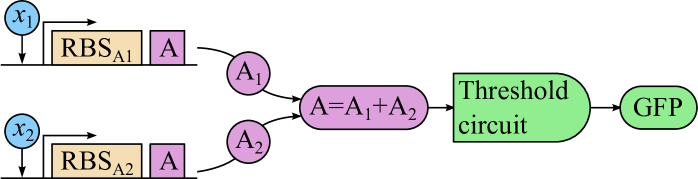
Figure 1: Scheme of a two-input linear classifier circuit. $x_{1}$, $x_{2}$ – inputs inducing the corresponding promoters, $\text{RBS}_{\text{A1}}$ and $\text{RBS}_{\text{A2}}$ – ribosome binding sites determining the strengths of the input branches, A – intermediate transcription factor (same in both input branches), GFP – reporter gene.

The stationary concentration $a$ of the intermediate transcription factor can be expressed as a weighted sum over all classifier inputs

$$a=\sum_{j}b_{j}a_{j}(x_{j}),$$ (1)

where $x_{j}$ are concentrations of the inputs $X_{j}$, $a_{j}(\cdot)$ are nonlinear functions, each describing the response to a particular input, including the whole appropriate signalling pathway, and $b_{j}$ are linear multipliers determining the relative strengths of the corresponding inputs, which can be varied in a range of more than $10^{5}$ fold by varying the DNA sequence within and near the ribosome binding site of the corresponding input gene [17, 18].

For a sharper discrimination between the classifier decisions, we propose to make use of the protein sequestration technique [25] to generate an ultrasensitive response to $A$ when its concentration exceeds a certain threshold. This is achieved by binding $A$, which normally induces the reporter gene, with a suitable inhibitor into an inactive complex which can not bind DNA. The simplest description of this binding assumes that free active transcription factor $A$ becomes available only when all inhibitor molecules are bound. Then the reporter protein concentration $g$ may be approximated by a shifted and truncated Hill function [25]

$$g=g(a;\theta)=\begin{cases}\alpha\gamma,&\mbox{if}\,a\leq\theta,\\ \gamma\frac{\alpha A_{g}+a-\theta}{A_{g}+a-\theta},&\mbox{if}\,a>\theta,\end{cases}$$ (2)

where $\theta$ is the threshold determined by the constitutive expression rate of the inhibitor [25], $A_{g}$ is the DNA-binding dissociation constant for $A$, $\gamma$ determines the maximal output, and $\alpha\gamma$ is the basal expression of the reporter protein in the absence of $A$.

A master population of cells with randomized individual response characteristics can be obtained by randomly varying the input weights $b_{j}$, as well as the threshold $\theta$, among the cells in the population. In the following we restrict ourselves to the case of two inputs, but our approach equally applies to input vectors of any dimension. We assume, that the parameter values in the $i$th individual cell are $b_{1}^{i}$ and $b_{2}^{i}$ for the input weights and $\theta^{i}$ for the threshold, the lower index denoting the input and the upper one labeling the cells, all other parameters being the same in both input channels in all cells.

The GFP output of a chosen $i$th individual classifier cell is then

$$f_{i}(x_{1},x_{2})=g(b_{1}^{i}a_{1}(x_{1})+b_{2}^{i}a_{2}(x_{2});\theta^{i})$$ (3)

with $g(a;\theta)$ defined in (2).

We use the discrete-output model of the individual cell to analyze the learning process and the distributed classifier behaviour. Namely, we assume, that each individual cell can produce two distinguishable kinds of output, corresponding to the cases in (2): low, or “negative answer” (which is the subthreshold background output $g_{i}=\alpha\gamma$), and high, or “positive answer” (above-threshold output).

We note, that each individual cell acts as a linear classifier in the transformed input space with coordinates $(a_{1},a_{2})$ defined by the corresponding nonlinear input functions

$$a_{1}=a_{1}(x_{1}),\quad a_{2}=a_{2}(x_{2}).$$ (4)

Indeed, an individual $i$th cell generates high output, when $b^{i}_{1}a_{1}+b^{i}_{2}a_{2}>\theta^{i}$, or

$$m_{1}^{i}a_{1}+m_{2}^{i}a_{2}>1,$$ (5)

where $m_{1,2}^{i}=b_{1,2}^{i}/\theta^{i}$.

Such classifier divides the transformed input space into two regions, corresponding to either answer of the classifier, which we will refer to as the negative and the positive classes. The border separating the classes in the transformed input space is a straight line

$$m^{i}_{1}a_{1}+m^{i}_{2}a_{2}=1.$$ (6)

Note, that $a_{1,2}$ as well as $m_{1,2}$ can not be negative due to their meaning. In the following, $a_{1,2}$ and $m_{1,2}$ are assumed to be non-negative real numbers. In particular it means, that the space of inputs and the space of parameters are always limited to the first quadrant of the full real space, regardless of its dimension.

Hard classification principle and learning strategy

An ensemble of linear classifiers can be utilized to perform a more complicated classification task with a piecewise-linear border in the transformed input space. Denote with $P_{i}$ the positive class of the $i$th individual classifier:

$$P_{i}=\left\{a_{1},a_{2}:m_{1}^{i}a_{1}+m_{2}^{i}a_{2}>1\right\}.$$ (7)

Let all elements in the ensemble be given the same input. Then the whole ensemble can be used as a single distributed classifier, dividing the transformed input space into the positive class $P=\bigcup_{i}P_{i}$, where at least one individual classifier gives the positive answer, and the negative class $D=\bar{P}=\bigcap_{i}\bar{P}_{i}$, where all classifiers answer negatively (here the bar “$\bar{\;}$” denotes complement in the transformed input space), see Fig. 2.

By construction, the negative class $D$ is entirely contained in each closed half-plane defined by any of its edges, which means it is always convex. The classification border is a polygonal line composed of segments, each described by an equation of type (6), all having negative slope, because both $m^{i}_{1}$ and $m^{i}_{2}$ are positive. In the limit of large number of cells, the negative class becomes a convex region bordered by the coordinate axes and a smooth classification border having negative tangent slope at each point.

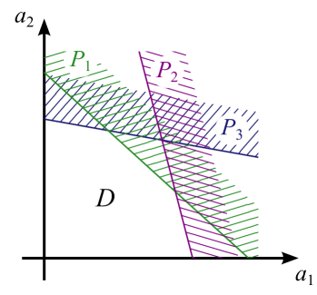
Figure 2: Hard classification principle. $P_{1}$, $P_{2}$, $P_{3}$ – positive classes of individual linear classifiers, $D$ – negative class of the collective classifier.

An ensemble constituting a distributed classifier with a specified (“target”) classification border (satisfying the requirements of negative slopes and convexity) can be prepared by the following learning algorithm. Let us start with a master population of linear classifiers of type (7) with random parameters $m_{1}^{i}$, $m_{2}^{i}$ distributed continuously over some interval. The aim of the learning is to keep all individual classifiers which answer correctly to all training examples and remove all incorrectly answering ones. To achieve this, we test the whole ensemble against a training sequence of samples from the negative class. All elements which answer positively to at least one negative sample are considered “incorrect” and are removed from the ensemble. This can be done, for example, using the fluorescence-activated cell sorting (FACS) technique. Positive class samples are not needed for learning, since hard classification fundamentally assumes separability of classes.

Actually, it is enough to use only samples located along the classification border. Although training sequences of this kind might be not available in real situations, theoretically, excluding the interior of the negative region from the training sequence leads to achieving the same learning outcome with a smaller number of samples.

The ensemble which remains after this learning procedure forms a distributed classifier with the class border determined by the training sequence. The actual set of cells constituting the trained distributed classifier is essentially the outcome of clipping the master population in the parameter space $(m_{1},m_{2})$ with a certain mask, which completely characterizes the action of the learning algorithm. In other words, the trained ensemble is a set intersection of the master population with a region in the parameter space, which we will refer to as the “trained ensemble region”.

To get an insight into a quantitative description of hard learning strategy, we start with a trivial case when the target classification border is linear, defined by the equation

$$\mu_{1}a_{1}+\mu_{2}a_{2}=1,$$ (8)

where $\mu_{1,2}$ are given constant coefficients, see Fig. 3 (a). Although this classification task can be solved by a single linear classifier, we use it as a starting point to describe the training of a distributed classifier.

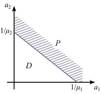
(a) (b)

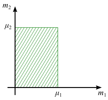
Figure 3: Training a distributed classifier with a linear target border. Panel (a). Target classes: $P$ – positive, $D$ – negative. Panel (b). Trained ensemble region on the plane of parameters: hatched area.

In the course of learning with a sequence of points distributed along the border (8), any element having $m_{1}>\mu_{1}$ or $m_{2}>\mu_{2}$ will eventually answer positively and therefore will be removed from the ensemble. Thus, the trained ensemble region on the plane $(m_{1},m_{2})$ is a rectangle (hatched area in Fig. 3 (b)).

Similarly, if the target border is a polygonal line (satisfying the requirements of negative slopes and convexity), with the target positive class being a union of several linear classes

$$P=\bigcup_{i}\left\{a_{1},a_{2}:\mu_{1}^{i}a_{1}+\mu_{2}^{i}a_{2}>1\right\},$$ (9)

where $\mu_{1}^{i}$, $\mu_{2}^{i}$ are the coefficients of the individual segments of the target polygonal border, then the trained ensemble region on the plane $(m_{1},m_{2})$ is a convex polygon with vertices $(\mu_{1}^{i},\mu_{2}^{i})$, shown in Fig. 9 (a) in Appendix S1 (see Supporting Information) as hatched area.

In Appendix S1 we analyze the response of a trained hard classifier to an input taken from the positive class. In particular, a lower estimate is obtained for the quantity of cells answering positively to such inputs. It is found to be proportional to the density of the master population per unit of the logarithmic parameter space $(\log m_{1},\log m_{2})$. It is also shown, that the maximal quantity $m_{\max}$, to which the region covered by the master population in the parameter space extends in both $m_{1}$ and $m_{2}$, should be not less than the inverse of the smaller intercept of the target class border (the intercepts are the abscissa and the ordinate of the points where the border crosses the axes $Oa_{1}$ and $Oa_{2}$).

Simulations

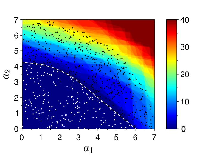
Figure 4: Simulation results for hard classification. Response of a trained distributed classifier in the space of inputs. Black-white dashed line – target (predefined) class border, white (black) filled circles – samples from the negative (positive) class, color – number of the positively responding cells (quantities 40 and above marked with same color).

To illustrate and verify the analytical results, we performed numerical simulations. We specify the class border (black-white dashed line in Fig. 4) composed of two sections. One section is a segment of the line $a_{1}+a_{2}=A$, and the other one is an arc of the circle $a_{1}^{2}+a_{2}^{2}=A^{2}/2$. The segments are connected at the point $a_{1}=a_{2}=A/2$, forming a smooth curve.

The negative class is the bounded part of the first quadrant of the plane $(a_{1},a_{2})$, separated by the border. The training sequence of length $N_{\text{train}}$ (white filled circles in Fig. 4) is randomly sampled from the negative class. The positive class is additionally bounded by condition $a_{1}^{2}+a_{2}^{2}<B^{2}$ with $B>A$.

The master population of the classifier cells is obtained by randomly sampling the parameters $(m_{1},m_{2})$ from the log-uniform distribution in the parameter space, bounded by the minimal and maximal values $m_{\min}$ and $m_{\max}$. The total number of cells in the master population is $N_{\text{master}}$. The uniform density of cells per logarithmic unit of the parameter space is

$$\alpha=\frac{N_{\text{master}}}{(\log m_{\max}-\log m_{\min})^{2}}.$$ (10)

The classifier is trained by presenting sequentially all training samples from the negative class, and discarding all cells answering positively to at least one sample. Algorithm description in Table 1 formalizes the above procedure.

In our simulation we let $N_{\text{master}}=300$, $N_{\text{train}}=200$, $A=6$, $B=8$. The smaller border intercept is $A/\sqrt{2}\approx 4.24$. In accordance to the criterion formulated in the end of the previous subsection, we let $m_{\max}=0.5>1/4.24$, and $m_{\min}=m_{\max}/100$. We measure the quantity of the positively responding cells of the trained classifier as a function of the input $(a_{1},a_{2})$. The result is depicted in Fig. 4 in color code. The straight interfaces of color, distinguishable in the figure, are the borders of type (6) associated with the individual linear classifiers (cells).

Soft classification problem

The approach considered above can only be applied to hard classification problems with a special type of the classification border (namely, the border must be a curve connecting the axes in the input space, having a negative slope at each point, with the negative class being a convex region, see subsection “Hard classification principle and learning strategy” for details). In order to address problems with classification border of more general type, or “soft” classification problems (i.e. problems with inseparable classes with a-priori unknown probability distributions in the input space) we employ soft learning strategy and a two-input elementary classifier design with a bell-shaped response function, which was suggested in [16].

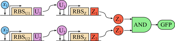
Figure 5: Scheme of a two-input classifier circuit with a bell-shaped response. $x_{1}$, $x_{2}$ – inputs inducing the corresponding promoters, $\text{RBS}_{\text{U1}}$ and $\text{RBS}_{\text{U2}}$ – ribosome binding sites determining the strengths of the input branches, $\text{U}_{1}$, $\text{U}_{2}$ – intermediate repressor/activator factors, $\text{Z}_{1}$, $\text{Z}_{2}$ – outputs of the individual branches, GFP – reporter gene.

Two-input classifier with a bell-shaped response

An elementary classifier circuit providing a bell-shaped response in the two-dimensional input space can be constructed of two independent sensing branches, whose outputs are combined using a genetic AND gate (Fig. 5) [16]. Each sensing branch is composed of two genetic modules, the sensor and the signal transducer [16]. The sensing module is monotonically induced by the corresponding input chemical signal $X_{j}$ ($j=1,2$) and drives the synthesis of an intermediate repressor/activator $U_{j}$. The signal transducer part is activated by $U_{j}$ at intermediate concentrations and inhibited at higher concentrations, providing the maximal response at a certain concentration level. The classic well-characterized example of such promoter is the promoter $P_{RM}$ of phage lambda which provides this kind of non-monotonic response to the lambda repressor protein CI [26].

The outputs $Z_{j}$ of both sensing branches drive the expression of a reporter protein (e.g., GFP) through a two-input genetic AND gate. A number of circuits performing logical operations including AND have been developed and characterized recently [22, 23, 24]. When each sensing branch provides a bell-shaped response function, then the response of the full circuit will also be a bell-shaped function in the two-dimensional input space.

Omitting the indices $j$ at all variables and parameters for the sake of conciseness and denoting the concentrations of $X$, $U$, $Z$ with $x$, $u$ and $z$, the steady-state concentration of each single sensing branch output $Z$ can be written as [16]

$$z(x;m_{u},m_{z})=\frac{r_{z}(r_{u}(x;m_{u})/\mu_{u};m_{z})}{\mu_{z}},$$ (11)

where $x$ is the input concentration, $\mu_{u}$ and $\mu_{z}$ are the degradation rates of $U$ and $Z$, respectively; $r_{u}(\cdot)$ and $r_{z}(\cdot)$ are the effective production rates of $U$ and $Z$ described by standard Hill functions

$$r_{u}(x;m_{u})=m_{u}\cdot\frac{\alpha A_{u}^{p_{u}}+x^{p_{u}}}{A_{u}^{p_{u}}+x^{p_{u}}},$$ (12)

$$r_{z}(u;m_{z})=m_{z}\cdot\frac{A_{z}^{p_{z}}u^{p_{z}}}{(A_{z}^{p_{z}}+u^{p_{z}})^{2}},$$ (13)

where $\alpha$ determines the basal expression from the sensor promoter in the absence of the input chemical $X$, $A_{u}$ and $A_{z}$ are the dissociation constants of $X$ and $U$ with their corresponding promoters, the Hill coefficients $p_{u}$ and $p_{z}$ characterize the cooperativity of activation or repression of the corresponding promoters, $m_{u}$ and $m_{z}$ describe the overall expression strength of $U$ and $Z$.

The function $z(x)$ defined by Eqs. (11)–(13) is bell-shaped in a range of $m_{u}/\mu_{u}\in(A_{z},A_{z}/\alpha)$, with the position of the maximum determined by the value of $m_{u}/\mu_{u}$ [16]. A master population of elementary two-input classifiers with response maxima randomly varied in the input space can be constructed by random variation of the sensory promoter strengths $m_{u}$ both among the individual cells, as well as among the two sensory branches in each cell. The variation range of the maximum position is limited by the parameter $\alpha$, which is for common promoters of the order of $10^{-3}$ [27, 28]. The full range can be covered, provided the promoter strengths $m_{u}$ are varied at least $1/\alpha=10^{3}$ fold, which is achievable, for example, by varying the DNA sequence within and near the ribosome binding site of the sensory gene [17, 18].

In the following we let the $m_{u}$ parameters of the two sensory branches in a chosen $i$th cell take on the values $m^{i}_{1}$ and $m^{i}_{2}$, the lower index denoting the input, the upper being the cell number, with all other parameters being the same in both sensory branches in all cells.

We model the AND gate, which drives the reporter protein production, as a product of two Hill functions

$$g(z_{1},z_{2})=\beta\cdot\frac{z_{1}^{p_{g}}}{A_{g}^{p_{g}}+z_{1}^{p_{g}}}\cdot\frac{z_{2}^{p_{g}}}{A_{g}^{p_{g}}+z_{2}^{p_{g}}},$$ (14)

where $z_{1,2}$ are the inputs to the AND gate, $\beta$ is a dimensional constant, $A_{g}$ and $p_{g}$ are respectively the dissociation constant and the Hill coefficient for the AND gate (for simplicity we assume equal values for both inputs).

The inputs to the AND gate are essentially the outputs of the sensory branches, thus the output of a chosen $i$th cell finally is

$$f_{i}(x_{1},x_{2})=g(z(x_{1};m^{i}_{1}),z(x_{2};m^{i}_{2})),$$ (15)

where $x_{1,2}$ are the classifier inputs, the function $g(\cdot,\cdot)$ is defined by (14), and $z(\cdot)$ by Eqs. (11)–(13) with $m_{u}$ substituted by $m^{i}_{1}$ or $m^{i}_{2}$ for either input branch, and index $i$ labeling the individual cells.

Soft learning strategy

By “soft learning” we mean a learning strategy which reshapes the population density in the parameter space in response to a sequence of training examples in order to maximize the correct answer probability for the distributed classifier taken as a whole, without any hard separation of the cells into “correct” and “incorrect”.

This can be achieved by organizing a kind of population dynamics which gives preference to cells which tend to maximize the performance of the whole classifier. In the simplest case, the training examples are sequentially presented to all cells in the population, and some cells get eliminated from the population in a probabilistic way, with survival probability depending upon the cell output, given the a-priori knowledge about the particular training example to belong to a certain class. This may be implemented by means of FACS technique.

We use a more elaborate learning strategy incorporating a mechanism for conserving the total cell count. In the model description this is achieved by simply replacing each discarded cell with a duplicate of a randomly chosen cell from the population. In experimental implementation the same effect can arise from the cell division process which goes on during the FACS cell selection. Alternatively, the proper competitive population dynamics can be organized by modulating the viabilities of the cells in accordance with the learning rule by means of e.g. antibiotic resistance genes controlled by the classifier circuit output in each individual cell.

In consistency with [16], we specify the probabilities of cell survival after presenting each training example as

$$p_{+}(g) =\frac{1}{1+\xi}+\frac{1}{1+\xi\exp(-g/\gamma)},$$ (16a)

$$p_{-}(g) =\frac{1}{1+\xi}-\frac{1}{1+\xi\exp(-g/\gamma)}+1,$$ (16b)

where $g$ is the cell output upon presenting a training example, $\xi=\exp((8\gamma^{-1}))$, $\gamma$ controls the “softness” of the learning (the greater $\gamma$, the softer is the slope of $p_{+}(g)$ and $p_{-}(g)$). Either $p_{+}(g)$ or $p_{-}(g)$ is used, depending on the class to which the training example is a-priori known to belong. The functions specified in (16a,b) have maximal slope at $g=1/8$. The cell output range should be scaled to cover this value by adjusting the constant $\beta$ in (14).

The output of a distributed classifier is the sum of all individual cell outputs:

$$f(x_{1},x_{2})=\sum_{i=1}^{N_{c}}f_{i}(x_{1},x_{2}),$$ (17)

where $f_{i}(x_{1},x_{2})$ is defined by (15), and $N_{c}$ is the total number of cells.

The classification decision is made by comparing the classifier output to a threshold $\theta$:

$$\mbox{decision}=\begin{cases}\mbox{``positive''},&\mbox{if}\,f(x_{1},x_{2})\geq\theta,\\ \mbox{``negative''},&\mbox{if}\,f(x_{1},x_{2})<\theta,\end{cases}$$ (18)

where $\theta$ has to be adjusted after the learning to maximize the correct answer rate of the classifier.

The classification border is actually a level line of $f(x_{1},x_{2})$ corresponding to the threshold $\theta$. The aim of the soft learning is thus to reshape the population and select the optimal value of $\theta$ in a way that the corresponding level line is the best approximation of the (unknown a-priori) optimal classification border. The computational criterion of this optimality is the maximization of the correct answer rate using the given training examples.

Simulations

We used algorithm described in Table 2 to implement the soft learning strategy. We demonstrate the use of the soft classification strategy to solve two problems which are not solvable with hard distributed classifiers described in section “Hard classification problem”. The first example has separable classes which consist of disjoint regions and thus do not satisfy the requirements of convexity and negative slopes which were imposed in subsection “Hard classification principle and learning strategy”. The positive class is specified as union of two circles on the $(x_{1},x_{2})$ plane, one centered at $x_{1}=x_{2}=A$ with radius $R$, and the other centered at $x_{1}=x_{2}=B$ with radius $3R$, and the negative class as union of two ellipses, one centered at $x_{1}=A$, $x_{2}=B$ with semiaxes $R$ and $3R$, and the other centered at $x_{1}=B$, $x_{2}=A$ with semiaxes $3R\sqrt{2}$ and $R\sqrt{2}$, where

$$R=\frac{1}{32}\left(1-10^{-1.5}\right),\quad A=10^{-1.5}+2R,\quad B=10^{-1.5}+8R.$$ (19)

The simulation parameters are $N_{c}=2\cdot 10^{3}$, $N_{\text{train}}=100$ (50 samples from each class), $N_{\text{iter}}=1000$, softness parameter $\gamma=0.4$, $m_{\min}=2^{2}A_{z}$, $m_{\max}=2^{8}A_{z}$, $A_{z}=20$, $m_{z}=A_{u}=1$, $A_{g}=2$, $p_{z}=p_{u}=p_{g}=2$, $\alpha=10^{-3}$. Output scaling constant $\beta=1056.25$ is chosen so that cell output $g$ ranges from 0 to 0.25 in consistency with expressions for survival probabilities (16a,b). The simulation result is presented in Fig. 6. All training samples are classified correctly after learning, but this becomes impossible in case of inseparable classification problems.

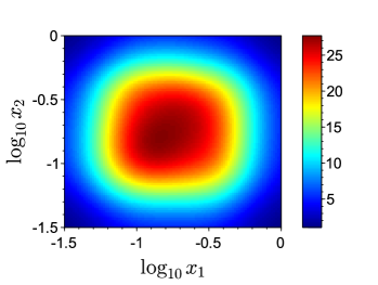
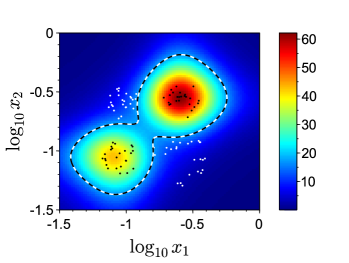
Figure 6: Simulation results for soft classification strategy applied to separable classes. Panel (a). Untrained (master) population output (color). Panel (b). Trained population output (color). White (black) filled circles – samples from the negative (positive) class, black-white dashed line – classification border of the trained classifier.

The next example shows the classifier operation for inseparable classes. For either class we use a two-dimensional log-normal distribution resulting from independently sampling both inputs $x_{1}$ and $x_{2}$ from a one-dimensional log-normal distribution centered at $\log_{10}x_{1,2}=-1.04$ for the positive class, and $\log_{10}x_{1,2}=-0.35$ for the negative class, with standard deviation of $\log_{10}x_{1,2}$ set to $0.22$. The number of training examples is $N_{\text{train}}=2000$ (1000 samples from each class). Other simulation parameters are the same as in the previous example. The result of the simulation is presented in Fig. 7 the same way as in the previous example.

Figure 7: Simulation results for soft classification strategy applied to inseparable classes. Notations same as in Fig. 6.

We compared the successful classification rates of our distributed gene classifier to that of several common machine learning algorithms [29] including the $k$-means method, support vector machine (SVM), and random forest algorithm, all implementations taken from the “scikit-learn” Python library [30] with default parameters. The comparison results are presented in Table 3. Simulation 1 is the same as in Fig. 7, and the only difference of Simulation 2 is the log-normal distribution’s central point location for the positive class, namely $\log_{10}x_{1,2}=-0.61$, which yields a greater overlap of the classes probability densities. The successful classification rates were computed using testing sequences of length $N_{\text{test}}=2000$ (1000 samples from each class), equal to that of the training sequences.

Discussion

In summary, in this paper we have presented a design of multi-input classifiers to be implemented as a synthetic genetic network. We have considered two examples, corresponding to hard and soft learning strategy. As a multi input classifier, these devices can solve classification task based on the data inseparable in the single dimension case. Moreover, the design developed allows to achieve practically arbitrary shape of the classification border in the space of input signals. Here we have considered two input genetic classifiers but the same design principles can be utilized to construct multi input classifying devices, then, the number of inputs is limited only by the number of possible hybrid promoters.

Our approach challenged a problem of discrimination between classes with overlapping probability density distributions in the input space. In this case the classification error probability cannot vanish and has to be minimized. The optimal solution to this problem is given by the Bayesian classification rule [31]. In case of equal a-priori probabilities for a randomly picked sample to belong to either class, the classification of a presented sample point from the parameter space is optimally done by comparing the class probability density functions at this point: the class with the greatest probability density value is the optimal answer to the classification problem. At the classification border the probability density functions get equal. If these functions are known a-priori, then the optimal border is thus also known, and the problem reduces to “hard classification” discussed above.

When the probability density functions of the classes are not known a-priori, the optimal classification rule is not known either, and the classifier has to be trained by examples. We will refer to this problem as “soft classification”. Hard learning is not applicable in this case, because it may lead eventually even to discarding all the cells. Inseparable classes with a-priori unknown probability density functions require another learning strategy which we will refer to as “soft learning”, when the decision to discard or to keep a particular cell upon presenting a training example is probabilistic, depending on the cell output.

An important aspect of synthetic biology is the design of smart biological devices or new intelligent drugs, through the development of in vivo digital circuits [32]. If living cells can be made to function as computers, one could envisage, for instance, the development of fully programmable microbial robots that are able to communicate with each other, with their environment and with human operators. These devices could then be used, e.g., for detection of hazardous substances or even to direct the growth of new tissue. In that direction, pioneering experimental studies have shown the feasibility of programmed pattern formation [9], the possibility of implementing logical gates and simple devices within cells [33], and the construction of new biological devices capable to solve or compute certain problems [34].

The classifiers designed could be considered as a further development towards the construction of robust and predictable synthetic genetic biosensors, which have the potential to affect and effect a lot of applications in the biomedical, therapeutic, diagnostic, bioremediation, energy-generation and industrial fields [35, 36, 37, 38].

Tables

Table 1: Hard learning algorithm

0:  Master population of $N_{\text{master}}$ elementary linear classifiers (cells) with parameters $(m_{1}^{i},m_{2}^{i})$ randomly sampled from the log-uniform distribution in the parameter space, bounded by the minimal and maximal values $m_{\min}$ and $m_{\max}$. The training sequence of negative class samples $(a_{1}^{j},a_{2}^{j})$ of length $N_{\text{train}}$.

0:  Trained set of cells constituting a distributed classifier.

  for each training sample $(a_{1}^{j},a_{2}^{j})$ do

     for each cell $i=1$ to $N_{\text{master}}$ do

        if (5) holds for this cell and this input (cell generates a positive answer) then

           Remove the cell from the ensemble.

        end if

     end for

  end for

Table 2: Soft learning algorithm

0:  Master population of $N_{c}$ elementary classifiers (cells) with bell-shaped output with parameters $(m_{1}^{i},m_{2}^{i})$ randomly sampled from the log-uniform distribution in the parameter space, bounded by the minimal and maximal values $m_{\min}$ and $m_{\max}$. The sequence of training examples $(x_{1}^{j},x_{2}^{j})$ of length $N_{\text{train}}$. The known class type $y^{j}=\pm 1$ for each example. The number of training iterations $N_{\text{iter}}$.

0:  Trained set of $N_{c}$ cells constituting a distributed classifier; classification threshold $\theta_{\text{opt}}$.

  for iteration $k=1$ to $N_{\text{iter}}$ do

     Choose a random example $(x_{1}^{j},x_{2}^{j})$.

     for each cell $i=1$ to $N_{c}$ do

        Calculate the $i$th cell output $g_{i}=f_{i}(x_{1}^{j},x_{2}^{j})$ according to (15).

        Calculate the cell survival probability according to (16a) or (16b): $p=p_{+}(g_{i})$ if $y_{i}=+1$, or $p=p_{-}(g_{i})$ if $y_{i}=-1$.

        With probability $1-p$, choose a random cell from the population and eliminate the $i$th cell, replacing it with the chosen cell.

     end for

  end for

  for each training example $j=1$ to $N_{\text{train}}$ do

     Use the trained population to calculate the population output $f(x_{1}^{j},x_{2}^{j})$ according to (17).

  end for

  Find the optimal classification threshold $\theta_{\text{opt}}$ by maximizing the correct classification rate over $\theta$: $\theta_{\text{opt}}=\text{argmax}\sum_{j=1}^{N_{\text{train}}}y^{j}\left[2H(f(x_{1}^{j},x_{2}^{j})-\theta)-1\right]$.

Table 3: Successful classification rate of the distributed gene classifier compared to that of other machine learning algorithms

	$k$-means	Support vector	Random forest	Distributed gene
		machine		classifier
Simulation 1	91.3	98.9	98.3	98.35
Simulation 2	71.45	80.75	79.3	77.1

Appendix S1. Deriving an estimate for hard classifier response

We assume, that the master population is characterized by a “working parameter domain” in the space of parameters $(m_{1},m_{2})$, such that the density of cells per logarithmic unit of the parameter space in this working domain is greater than or equal to a known minimal value $\alpha$. Precisely, we assume, that the expected number of cells $dN$ falling within a parameter space element $dm_{1}dm_{2}$ satisfies the following inequality everywhere in the working parameter domain:

$$dN\geq\alpha\cdot d(\log m_{1})\,d(\log m_{2}).$$ (20)

Below we derive a lower estimate for $N_{pos}(a_{1}^{\text{in}},a_{2}^{\text{in}})$ which is the expectation of the number of cells answering positively to an input $(a_{1}^{\text{in}},a_{2}^{\text{in}})$ taken from the positive class:

$$N_{pos}(a_{1}^{\text{in}},a_{2}^{\text{in}})>\frac{2\alpha\delta^{2}}{(1+\delta)^{2}},$$ (21)

where $\delta$ is a parameter determining the offset of the input from the classification border into the positive class. In general, $\delta$ is defined in a way that $(1+\delta)$ is a factor by which the negative region has to be scaled so as its border reaches the input point (see details below). Using polar coordinates $(\rho,\phi)$ defined by $a_{1}=\rho\cos\phi$, $a_{2}=\rho\sin\phi$, we can define $\delta$ in the form

$$\delta=\frac{\rho^{\text{in}}}{\rho_{b}(\phi^{\text{in}})}-1,$$ (22)

where $\rho=\rho_{b}(\phi)$ is the border equation, and $(\rho^{\text{in}},\phi^{\text{in}})$ is the input point:

$$\begin{split}a_{1}^{\text{in}}&=\rho^{\text{in}}\cos\phi^{\text{in}},\\ a_{2}^{\text{in}}&=\rho^{\text{in}}\sin\phi^{\text{in}}.\end{split}$$ (23)

The derivation of (21) is based upon the assumption that the whole region of the parameter space associated with producing the positive output of the trained classifier is contained in the working parameter domain, and hence is populated by cells with density satisfying (20). This is actually the only requirement limiting the applicability of (21).

Below we analyze this requirement in case of the working parameter domain specified as a rectangle $\{m_{\min}\leq m_{1,2}\leq m_{\max}\}$. We derive a set of conditions providing the applicability of (21) to a particular input $(a_{1}^{\text{in}},a_{2}^{\text{in}})$:

$$\mu_{1}^{\ast}\leq m_{\max},\quad\mu_{2}^{\ast}\leq m_{\max},$$ (24a)

$$m_{\min}a_{1}^{\text{in}}+\mu_{2}^{\ast}a_{2}^{\text{in}} \leq 1,$$ (24b)

$$\mu_{1}^{\ast}a_{1}^{\text{in}}+m_{\min}a_{2}^{\text{in}} \leq 1.$$ (24c)

with $\mu_{1}^{\ast}$ and $\mu_{2}^{\ast}$ defined as the coefficients of an equation in the form (8), describing the tangent to the border drawn at the point where it is crossed by the input’s radius vector.

Conditions (24a-c) are given a geometrical interpretation and can be used for choosing parameter values in experiment and simulations. Condition (24a) can be formulated in terms of the border intercepts (the abscissa and the ordinate of the points where the border crosses the axes). Namely, $m_{\max}$ should not be less than the inverse of each intercept. The interpretation of (24b,c) is less straightforward, but it suggests that these conditions fail whenever the input point is too close to either axis, or the tangent to the border drawn at the point where it is crossed by the input radius vector is too close to being parallel to either axis. At the same time, (24b,c) are the less likely to fail, the smaller is $m_{\min}$, and the closer is the input to the border (which implies smaller $\delta$).

We stress that the lower estimate in (21) is obtained for expectations, and the actual count of the positively answering cells is a random variate determined by a particular realization (scattering) of the master population in the parameter space.

To validate the estimate (21), we extended the simulation described in section “Hard classification problem” by testing the trained classifier against a sequence of $N_{\text{test}}=500$ samples from the positive class (black filled circles in Fig. 4). For each input $(a_{1}^{\text{in}},a_{2}^{\text{in}})$ we calculate the corresponding $\delta$ according to (22), (23), and measure the quantity of the positively responding cells $N_{\text{pos}}(a_{1}^{\text{in}},a_{2}^{\text{in}})$. The obtained set of pairs $N_{\text{pos}}$ versus $\delta$ is plotted with red filled circles in Fig. 8. The analytical lower estimate (21) is plotted with a blue dashed line.

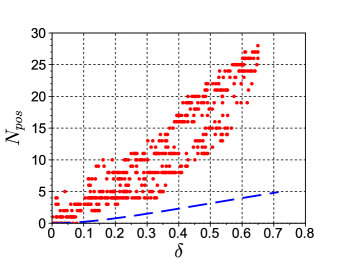
Figure 8: Validating the estimate for hard classifier response. Number of positively responding cells $N_{pos}$ versus the input offset $\delta$ from the class border. Red circles – simulation results, blue dashed line – lower estimate (21).

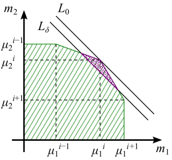
(a) (b)

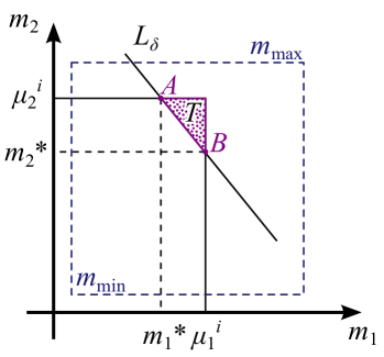
Figure 9: Estimating the number of positively responding cells. Panel (a). Hatched area – trained ensemble region, dotted area – cells answering positively to an input sample from the positive class. Panel (b). Dashed square – working parameter domain. Other notations – see text.

In order to derive (21), we first notice, that each particular input $(\tilde{a}_{1},\tilde{a}_{2})$ can be associated with a straight line on the parameter plane $(m_{1},m_{2})$, defined by the equation

$$m_{1}\tilde{a}_{1}+m_{2}\tilde{a}_{2}=1.$$ (25)

Consider a polygonal classification border (satisfying the requirements of negative slopes and convexity) and an input $(a_{1}^{0},a_{2}^{0})$ lying exactly on the border, namely, on its $i$th segment, and satisfying the $i$th segment’s equation:

$$\mu_{1}^{i}a_{1}^{0}+\mu_{2}^{i}a_{2}^{0}=1.$$ (26)

The corresponding line $L_{0}$ defined by (25) with $\tilde{a}_{1}=a_{1}^{0}$, $\tilde{a}_{2}=a_{2}^{0}$ then touches the trained ensemble region on the parameter plane at the vertex $(\mu_{1}^{i},\mu_{2}^{i})$ (Fig. 9 (a)).

Now consider another input $(a_{1}^{\text{in}},a_{2}^{\text{in}})$, which is slightly shifted from the border into the positive class, namely, satisfying

$$\mu_{1}^{i}a_{1}^{\text{in}}+\mu_{2}^{i}a_{2}^{\text{in}}=1+\delta,$$ (27)

where $\delta>0$ is a parameter determining the offset of the input point from the negative class. The line $L_{\delta}$ defined by (25) with $\tilde{a}_{1}=a_{1}^{\text{in}}$, $\tilde{a}_{2}=a_{2}^{\text{in}}$ then crosses the trained ensemble region (Fig. 9 (a)).

Let us estimate the expectation $N_{pos}(a_{1}^{\text{in}},a_{2}^{\text{in}})$ of the number of cells in the trained ensemble which answer positively to the input $(a_{1}^{\text{in}},a_{2}^{\text{in}})$. We note, that the individual cells answering positively to this input are exactly those, whose parameters are located in the trained ensemble region above the line $L_{\delta}$ (dotted area in Fig. 9 (a)).

We also notice, that the rectangle $\{0<m_{1}\leq\mu_{1}^{i},0<m_{2}\leq\mu_{2}^{i}\}$ is always a subset of the trained ensemble region (see Fig. 9 (a)). Denote with $T$ a piece of this rectangle which is cut from it by the line $L_{\delta}$ (dotted area in Fig. 9 (b)):

$$T=\left\{m_{1},m_{2}:0<m_{1}\leq\mu_{1}^{i},0<m_{2}\leq\mu_{2}^{i},m_{1}a_{1}^{\text{in}}+m_{2}a_{2}^{\text{in}}>1\right\}.$$ (28)

Denoting the expectation of the cell count in $T$ with $N_{T}(a_{1}^{\text{in}},a_{2}^{\text{in}})$, we observe that it is a lower estimate for $N_{pos}(a_{1}^{\text{in}},a_{2}^{\text{in}})$:

$$N_{pos}(a_{1}^{\text{in}},a_{2}^{\text{in}})\geq N_{T}(a_{1}^{\text{in}},a_{2}^{\text{in}}).$$ (29)

We consider the case when $T$ is a triangle (not a trapezium) and justify this assumption below.

We express $N_{T}(a_{1}^{\text{in}},a_{2}^{\text{in}})$ as an integral

$$N_{T}(a_{1}^{\text{in}},a_{2}^{\text{in}})=\int_{T}f(m_{1},m_{2})\,dm_{1}dm_{2},$$ (30)

where $f(m_{1},m_{2})$ is the “cell density function” in the parameter space $(m_{1},m_{2})$. Since the minimal cell density $\alpha$ in the logarithmic parameter space is specified by (20), the cell density function satisfies

$$f(m_{1},m_{2})\geq\frac{\alpha}{m_{1}m_{2}},$$ (31)

as soon as the pair $(m_{1},m_{2})$ belongs to the working parameter domain. We assume, that (31) holds in the whole area of $T$ and provide a sufficient condition for this below.

As $f(m_{1},m_{2})$ in (31) is falling in both arguments, the integral in (30) can be given a lower estimate

$$N_{T}(a_{1}^{\text{in}},a_{2}^{\text{in}})>f(\mu_{1}^{i},\mu_{2}^{i})\cdot S(T)\geq\frac{\alpha\delta^{2}}{2\mu_{1}^{i}\mu_{2}^{i}a_{1}^{\text{in}}a_{2}^{\text{in}}},$$ (32)

where $S(T)={\delta^{2}}/{(2a_{1}^{\text{in}}a_{2}^{\text{in}})}$ is the area of the triangle $T$. Taking into account the inequality of arithmetic and geometric means, which along with (27) yields

$$\mu_{1}^{i}\mu_{2}^{i}a_{1}^{\text{in}}a_{2}^{\text{in}}\leq(\mu_{1}^{i}a_{1}^{\text{in}}+\mu_{2}^{i}a_{2}^{\text{in}})^{2}/4=(1+\delta)^{2}/4,$$

and combining (32) with (29), we finally arrive at (21).

The input offset parameter $\delta$ is introduced in (27). Geometrically, the input point $(a_{1}^{\text{in}},a_{2}^{\text{in}})$ is located on a straight line which results from scaling the line drawn through the $i$th border segment (defined by (26)) by a factor of $(1+\delta)$ with the transform center placed at the origin of the coordinates. This could be used as a definition for $\delta$, but the choice of the “$i$th segment” itself may be ambiguous. However, the calculation remains valid regardless of this particular choice. To obtain the best (highest) estimation in (21), we should choose the segment number $i$ which maximizes $\delta$ in (27) for a given input.

To solve this maximization problem, consider a uniform scaling of the negative region (with the transform center at the coordinates origin) by a factor of $s$, such that the input point $(a_{1}^{\text{in}},a_{2}^{\text{in}})$ becomes located on the scaled class border (the negative class is “inflated” till it reaches the input point). Denote with $l$ the number of the border segment, which hits the input point when the border is scaled. It means, that the following equation is satisfied:

$$\frac{\mu_{1}^{l}}{s}a_{1}^{\text{in}}+\frac{\mu_{2}^{l}}{s}a_{2}^{\text{in}}=1.$$ (33)

At the same time, due to the convexity of the negative region, for all segments of the scaled border the following inequality holds:

$$\frac{\mu_{1}^{i}}{s}a_{1}^{\text{in}}+\frac{\mu_{2}^{i}}{s}a_{2}^{\text{in}}\leq 1$$ (34)

with the equality taking place only for $i=l$ and, in the special case when the input hits a vertex of the scaled polygon, for two adjacent segments. Comparing (33) and (34) to (27) we conclude, that $\delta$ in (27) is maximized at $i=l$, and this maximal value satisfies $1+\delta=s$. Essentially, the “optimal” segment $i=l$ is the one which is crossed by the input’s radius vector (or just a straight line segment drawn from the coordinates origin to the input point).

Thus, for an arbitrary given polygonal classification border (satisfying the requirements of convexity and negative slopes) the best estimate in (21) is obtained, when $\delta$ is defined in a way that $(1+\delta)$ is a factor by which the negative region has to be “inflated” (i.e. scaled up in the transformed input space $(a_{1},a_{2})$ with the origin of the coordinates used as the scaling transform center), so as the input point finds itself on the scaled classification border. This definition of $\delta$ remains equally valid in the limit of a smooth border. Using polar coordinates, we can express this definition in the form (22).

In the derivation of (21) exactly two assumptions were made: (i) $T$ being a triangle, and (ii) cell density estimation (31) valid in the whole area of $T$. Let us check their applicability for a given input $(a_{1}^{\text{in}},a_{2}^{\text{in}})$.

In case of a polygonal border, denote with $\mu_{1,2}^{\ast}=\mu_{1,2}^{l}$ the equation coefficients of the “optimal” border segment $i=l$ (crossed by the input’s radius vector), identified in (33). In the smooth border limit, instead of the optimal border segment one can speak of the “optimal” border tangent, drawn at the point where the border is crossed by the input’s radius vector. In this case we denote with $\mu_{1,2}^{\ast}$ the equation coefficients of this optimal tangent.

Denote with $m_{1}^{\ast}$ the value of $m_{1}$ at the crossing point of the lines $L_{\delta}$ and $m_{2}=\mu_{2}^{\ast}$ (i.e., abscissa of the point $A$ in Fig. 9(b)), and with $m_{2}^{\ast}$ the value of $m_{2}$ at the crossing point of the lines $L_{\delta}$ and $m_{1}=\mu_{1}^{\ast}$ (i.e., ordinate of $B$ in Fig. 9(b) ):

$$m_{1}^{\ast}=\frac{1-\mu_{2}^{\ast}a_{2}^{\text{in}}}{a_{1}^{\text{in}}},\quad m_{2}^{\ast}=\frac{1-\mu_{1}^{\ast}a_{1}^{\text{in}}}{a_{2}^{\text{in}}}.$$ (35)

Assume, that the working parameter domain (where (31) holds) is specified as a rectangle $\{m_{\min}\leq m_{1,2}\leq m_{\max}\}$. Using the above notations, we write down the conditions

$$\mu_{1}^{\ast} \leq m_{\max}, \quad\mu_{2}^{\ast} \leq m_{\max},$$ (36)

$$m_{1}^{\ast} \geq m_{\min}, \quad m_{2}^{\ast} \geq m_{\min},$$ (37)

which provide that $T$ is a subset of the working parameter domain, and a corollary fact is $T$ being a triangle (since $m_{1,2}^{\ast}>0$ automatically). Inserting (35) into (37), we rewrite it in the form

$$\begin{split}m_{\min}a_{1}^{\text{in}}+\mu_{2}^{\ast}a_{2}^{\text{in}}&\leq 1,\\ \mu_{1}^{\ast}a_{1}^{\text{in}}+m_{\min}a_{2}^{\text{in}}&\leq 1.\end{split}$$ (38)

Combining (36) with (38) yields the set of conditions (24a-c).

These conditions can be given a geometrical interpretation. Rewriting the equation of a border tangent in the intercept form instead of the form (8) yields the intercepts of the tangent (the abscissa and the ordinate of the points where it crosses the axes), which are $1/\mu_{1}^{\ast}$ and $1/\mu_{2}^{\ast}$. The minimal values of these intercepts are actually the intercepts of the border itself (due to convexity). Therefore, the maximal values of $\mu_{1}^{\ast}$ and $\mu_{2}^{\ast}$ can be found as the inverse of the border intercepts. Condition (36) then reduces to the requirement that $m_{max}$ should not be less than the inverse of each intercept.

The interpretation of (38) is less straightforward. Consider the point where the class border is crossed by the input’s radius vector, and the border tangent drawn at this point, earlier referred to as the “optimal tangent”, whose equation coefficients are $\mu_{1}^{\ast}$ and $\mu_{2}^{\ast}$. Denote with $d$ the length of the tangent segment belonging to the first quadrant and clipped by the axes. This segment is split into two sections by the tangency point. Denote with $d_{1}$ and $d_{2}$ the lengths of these sections adjacent to the axes $Oa_{1}$ and $Oa_{2}$, respectively, so that $d=d_{1}+d_{2}$. Then a geometrical calculation yields

$$\mu_{1}^{\ast}a_{1}^{\text{in}}=(1+\delta)\frac{d_{2}}{d},\quad\mu_{2}^{\ast}a_{2}^{\text{in}}=(1+\delta)\frac{d_{1}}{d}.$$ (39)

Inserting (39) into (38), we obtain

$$\begin{split}m_{\min}a_{1}^{\text{in}}+\delta&\leq\frac{d_{2}}{d}(1+\delta),\\ m_{\min}a_{2}^{\text{in}}+\delta&\leq\frac{d_{1}}{d}(1+\delta).\end{split}$$ (40)

This condition favors smaller $\delta$ and $m_{\min}$, but fails whenever $d_{1}/d$ or $d_{2}/d$ becomes too small. This is the case, when the input is close to either axis, or the tangent to the border drawn at the point where it is crossed by the input radius vector is too close to being parallel to either axis.

References

- 1. Gardner TS, Cantor CR, Collins JJ (2000) Construction of a genetic toggle switch in escherichia coli. Nature 403: 339-42.
- 2. Elowitz MB, Leibler S (2000) A synthetic oscillatory network of transcriptional regulators. Nature 403: 335-8.
- 3. Stricker J, Cookson S, Bennett MR, Mather WH, Tsimring LS, et al. (2008) A fast, robust and tunable synthetic gene oscillator. Nature 456: 516-9.
- 4. Tigges M, Marquez-Lago TT, Stelling J, Fussenegger M (2009) A tunable synthetic mammalian oscillator. Nature 457: 309-12.
- 5. Fung E, Wong WW, Suen JK, Bulter T, Lee SG, et al. (2005) A synthetic gene-metabolic oscillator. Nature 435: 118-22.
- 6. Danino T, Mondragon-Palomino O, Tsimring L, Hasty J (2010) A synchronized quorum of genetic clocks. Nature 463: 326-30.
- 7. Kim J, Winfree E (2011) Synthetic in vitro transcriptional oscillators. Mol Syst Biol 7: 465.
- 8. Friedland AE, Lu TK, Wang X, Shi D, Church G, et al. (2009) Synthetic gene networks that count. Science 324: 1199-202.
- 9. Basu S, Gerchman Y, Collins CH, Arnold FH, Weiss R (2005) A synthetic multicellular system for programmed pattern formation. Nature 434: 1130-4.
- 10. Fernando CT, Liekens AM, Bingle LE, Beck C, Lenser T, et al. (2009) Molecular circuits for associative learning in single-celled organisms. J R Soc Interface 6: 463-9.
- 11. Levskaya A, Chevalier AA, Tabor JJ, Simpson ZB, Lavery LA, et al. (2005) Synthetic biology: engineering escherichia coli to see light. Nature 438: 441-2.
- 12. Bonnet J, Subsoontorn P, Endy D (2012) Rewritable digital data storage in live cells via engineered control of recombination directionality. Proc Natl Acad Sci U S A 109: 8884-9.
- 13. Tamsir A, Tabor JJ, Voigt CA (2011) Robust multicellular computing using genetically encoded nor gates and chemical ’wires’. Nature 469: 212-5.
- 14. Bonnet J, Yin P, Ortiz ME, Subsoontorn P, Endy D (2013) Amplifying genetic logic gates. Science 340: 599-603.
- 15. Siuti P, Yazbek J, Lu TK (2013) Synthetic circuits integrating logic and memory in living cells. Nat Biotechnol 31: 448-52.
- 16. Didovyk A, Kanakov OI, Ivanchenko MV, Hasty J, Huerta R, et al. (submitted 2014) Distributed classifier based on genetically engineered bacterial cell cultures. ACS Synthetic Biology .
- 17. Salis HM, Mirsky EA, Voigt CA (2009) Automated design of synthetic ribosome binding sites to control protein expression. Nature biotechnology 27: 946–950.
- 18. Kudla G, Murray AW, Tollervey D, Plotkin JB (2009) Coding-sequence determinants of gene expression in escherichia coli. science 324: 255–258.
- 19. Pfleger BF, Pitera DJ, Smolke CD, Keasling JD (2006) Combinatorial engineering of intergenic regions in operons tunes expression of multiple genes. Nature biotechnology 24: 1027–1032.
- 20. Wang HH, Isaacs FJ, Carr PA, Sun ZZ, Xu G, et al. (2009) Programming cells by multiplex genome engineering and accelerated evolution. Nature 460: 894–898.
- 21. Zelcbuch L, Antonovsky N, Bar-Even A, Levin-Karp A, Barenholz U, et al. (2013) Spanning high-dimensional expression space using ribosome-binding site combinatorics. Nucleic acids research 41: e98–e98.
- 22. Wang B, Kitney RI, Joly N, Buck M (2011) Engineering modular and orthogonal genetic logic gates for robust digital-like synthetic biology. Nature communications 2: 508.
- 23. Moon TS, Lou C, Tamsir A, Stanton BC, Voigt CA (2012) Genetic programs constructed from layered logic gates in single cells. Nature 491: 249–253.
- 24. Shis DL, Bennett MR (2013) Library of synthetic transcriptional AND gates built with split T7 RNA polymerase mutants. Proceedings of the National Academy of Sciences 110: 5028–5033.
- 25. Buchler NE, Cross FR (2009) Protein sequestration generates a flexible ultrasensitive response in a genetic network. Molecular systems biology 5.
- 26. Ptashne M (1986) A genetic switch: Gene control and phage lambda. Palo Alto, CA (US); Blackwell Scientific Publications.
- 27. Lutz R, Bujard H (1997) Independent and tight regulation of transcriptional units in Escherichia coli via the LacR/O, the TetR/O and AraC/– regulatory elements. Nucleic acids research 25: 1203–1210.
- 28. Cox RS, Surette MG, Elowitz MB (2007) Programming gene expression with combinatorial promoters. Molecular systems biology 3.
- 29. Hastie T, Tibshirani R, Friedman J (2009) The elements of statistical learning. Data Mining, Inference, and Prediction. Springer Series in Statistics. Springer, 2nd edition.
- 30. Pedregosa F, Varoquaux G, Gramfort A, Michel V, Thirion B, et al. (2011) Scikit-learn: Machine learning in Python. The Journal of Machine Learning Research 12: 2825–2830.
- 31. Duda RO, Hart PE, Stork DG (2012) Pattern classification. John Wiley & Sons.
- 32. Weiss R, Homsy GE, Knight TF (2002) Toward in vivo digital circuits. Evolution as Computation : 275-295.
- 33. Moon TS, Lou CB, Tamsir A, Stanton BC, Voigt CA (2012) Genetic programs constructed from layered logic gates in single cells. Nature 491: 249-253.
- 34. Haynes KA, Silver PA (2009) Eukaryotic systems broaden the scope of synthetic biology. J Cell Biol 187: 589-96.
- 35. Lu TK, Khalil AS, Collins JJ (2009) Next-generation synthetic gene networks. Nat Biotechnol 27: 1139-50.
- 36. Khalil AS, Collins JJ (2010) Synthetic biology: applications come of age. Nat Rev Genet 11: 367-79.
- 37. Ruder WC, Lu T, Collins JJ (2011) Synthetic biology moving into the clinic. Science 333: 1248-52.
- 38. Weber W, Fussenegger M (2012) Emerging biomedical applications of synthetic biology. Nat Rev Genet 13: 21-35.