Variational approach to multidimensional solitons in highly nonlocal nonlinear media

Abstract

We apply the variational approach to solitons in highly nonlocal nonlinear media in $D=1,2,3$ dimensions. We compare results obtained by the variational approach with those obtained in the accessible soliton approximation, by considering the same system of equations in the same spatial region and under the same boundary conditions. To assess the accuracy of these approximations, we also compare them with the numerical solution of the equations. We discover that the variational highly nonlocal approximation provides more accurate results and as such is more appropriate solution than the accessible soliton approximation.

I Introduction

Optical spatial solitons are self-localized wave packets that propagate in a nonlinear medium without changing their structure Kivshar and Agrawal (2003). This is made possible by the robust balance between dispersion and nonlinearity or between diffraction and nonlinearity or between all three effects in the propagation of spatiotemporal localized optical fields. An important characteristic of real nonlinear media is their nonlocality, that is, the fact that characteristic size of the response of the medium is wider than the size of the excitation itself. Strong nonlocality is of special interest, because it is observed in many media. For example, in nematic liquid crystals (NLCs) both experimental and theoretical studies indicated that the nonlinearity is highly nonlocal – meaning that the size of response is much wider than the size of excitation Henninot et al. (2007); Hutsebaut et al. (2005); Beeckman et al. (2004).

In 1997, Snyder and Mitchell introduced a model of nonlinearity whose response is highly nonlocal Snyder and Mitchell (1997) – in fact, infinitely nonlocal. They proposed an elegant theoretical model, intimately connected with the linear harmonic oscillator, that described complex soliton dynamics in simple terms, even in two and three dimensions. Because of the simplicity of the theory, they coined the term ”accessible solitons” (ASs) for these optical spatial solitary waves. However, straightforward application of the AS theory, even in nonlinear media with almost infinite range of nonlocality, inevitably led to additional problems Conti et al. (2003, 2004); Henninot et al. (2008), because there exists no real physical medium without boundaries and without noise.

To include interactions between solitons within boundaries, as well the impact of the finite size of the sample, we developed a variational approach (VA) to solitons in nonlinear media with long-range nonlocality, such as NLCs Aleksić et al. (2012), materials with thermal nonlocality Buccoliero et al. (2009), photo-refractive crystals Belić et al. (2002), and Bose-Einstein condensates Santos et al. (2003). Starting from an appropriate ansatz, this approach delivers a stationary solution for the beam amplitude and width, as well as the period of small oscillations about the stationary state. It provides for natural explanation of oscillations seen when, e.g., noise is included into the nonlocal nonlinear models. The noise is inevitable in any real physical system and causes a regular oscillation of soliton parameters with the period well predicted by our VA calculus Aleksić et al. (2012). It may even destroy solitons Petrović et al. (2013). Although our VA results were corroborated by numerics and experiments, they still attracted a heated exchange with other researchers Assanto and Smyth (2013); Aleksić et al. (2013). We have investigated in detail the destructive influence of noise on the shape-invariant solitons in a highly nonlocal NLCs in Petrović et al. (2013).

Owing to great impact and practical relevance of the AS model, in this paper we systematically compare it with the VA approximation in highly nonlocal nonlinear media in $D=1,2,3$ dimensions. We consider both systems using the same general equations, in the same spatial region, and under the same boundary conditions. To check the accuracy of both approximations, we compare them with the numerical solution of the equations. We find that multidimensional variational highly nonlocal approximation provides very accurate results, while the beam parameters obtained by using the AS approximation show systematic and predictable discrepancy with numerical results.

The paper is organized in the following manner. In Sec. 2 we introduce the model, Sec. 3 presents results obtained by the variational approach, Sec. 4 discusses the accessible soliton approximation, Sec. 5 presents numerical results, and Sec. 6 brings conclusions.

II The model

For the study of VA and AS approximations to the fundamental soliton solutions in a ($D$+1)-dimensional highly nonlocal medium we adopt the following model of coupled dimensionless equations Kivshar and Agrawal (2003); Aleksić et al. (2012):

$$2i{\frac{\partial E}{\partial z}}+\Delta E+\theta E=0,$$ (1)

$$2\Delta\theta-\alpha\theta+\left|E\right|^{2}=0,$$ (2)

with zero boundary conditions on a $D$-dimensional sphere $\left(D=1,2,3\right)$. Here $\Delta$ is the $D$-dimensional Laplacian. The system of equations of interest consists of the nonlinear Schrödinger equation for the propagation of the optical field $E$ and the diffusion equation for the nonlocal response of the medium $\theta$. This is a fairly general model for nonlinear optical media with diffusive nonlocality, widely used in the literature Kivshar and Agrawal (2003); Conti et al. (2003); Aleksić et al. (2012). In the local limit, the first term in Eq. (2) can be neglected and the model reduces to the Schrödinger equation with Kerr nonlinearity. In the opposite limit, the second term in Eq. (2) can be neglected and the highly nonlocal model is reached. Since we are interested in the strong nonlocality, we will omit in our analysis the $\alpha$ term from Eq. (2).

For radially-symmetric intensity distributions $\left|E\right|^{2}$, Eq. (2) can be solved using Green’s functions,

$$\theta_{D}(r)=\frac{1}{2}\int G_{D}(r,\rho)\left|E(\rho)\right|^{2}\rho^{D-1}d\rho,$$ (3)

where $G_{D}(r,\rho)$  is the Green’s function in $D$ dimensions, defined as follows:

$$G_{D}(r,\rho)=\left\{\begin{array}[]{c}\left(r^{2-D}-d^{2-D}\right)/(D-2),\qquad\rho<r<d\\ \left(\rho^{2-D}-d^{2-D}\right)/(D-2),\qquad r<\rho<d\end{array}\right\}.$$ (4)

Here $d$ is some characteristic transverse distance of interest. In the two-dimensional case (here and thereafter), the limit $D\rightarrow 2$ should be taken, leading to

$$G_{2}(r,\rho)=\left\{\begin{array}[]{c}\ln\left(r/d\right),\qquad\rho<r<d\\ \ln\left(\rho/d\right),\qquad r<\rho<d\end{array}\right\}.$$ (5)

For the Gaussian-shaped beams with the field intensity:

$$\left|E(r)\right|^{2}=\frac{Q_{D}}{T^{D}\pi^{D/2}}\exp\left(-\frac{r^{2}}{T^{2}}\right),$$ (6)

the solution of Eq. (3) can be written as

$$\begin{split}\theta_{D}(r)=\frac{Q_{D}}{4\pi^{D/2}(2-D)}\left\{r^{2-D}\Gamma(D/2,r^{2}/T^{2})-\right.\\ \left.T^{2-D}\exp(-r^{2}/T^{2})+\left[d^{2-D}-r^{2-D}\right]\Gamma(D/2)\right\}+O(\delta),\end{split}$$ (7)

where $\delta=\max\{\exp(-d^{2}/T^{2})\}\ll 1$ and $T$ is the characteristic width of the optical field. The $D-$dimensional power is given by $Q_{D}=\nu\int\left|E\right|^{2}r^{D-1}dr$, where $\nu=2\pi^{D/2}/\Gamma(D/2)$.

In an explicit form for different dimensions, Eq. (7) yields:

$$\theta_{1}(r)=\frac{Q_{1}}{4}\left[d-r\operatorname{erf}\left(\frac{r}{T}\right)-\frac{T\exp(-r^{2}/T^{2})}{\sqrt{\pi}}\right]+O(\delta),$$ (8)

$$\theta_{2}(r)=\frac{Q_{2}}{8\pi}\left[\operatorname{E_{i}}\left(-\frac{r^{2}}{T^{2}}\right)-\ln\left(\frac{r^{2}}{d^{2}}\right)\right]+O(\delta),$$ (9)

$$\theta_{3}(r)=\frac{Q_{3}}{8\pi}\left[\frac{\operatorname{erf}\left(r/T\right)}{r}-\frac{1}{d}\right]+O(\delta),$$ (10)

for one, two, and three dimensions, respectively.

In the equations above, $\operatorname{erf}(z)=\left(2/\sqrt{\pi}\right)\int_{0}^{z}\exp(-t^{2})dt$ is the error function, $Ei=-\int_{-z}^{\infty}t^{-1}\exp(-t)dt$ is the exponential integral function, $\Gamma(z)=\int_{0}^{\infty}t^{z}\exp(-t)dt$ is the Euler gamma function, and $\Gamma(a,z)=\int_{z}^{\infty}t^{a-1}\exp(-t)dt$ is the incomplete gamma function Abramowitz and Stegun (1964). The form of $\theta$ corresponds to a radially-symmetric solution of Eq. (2), with zero boundary conditions on a circle of radius $d\gg T$, and in the limit of a thick transverse width. We can take these expressions as an approximate solution on a $D-$dimensional cube, as demonstrated in Aleksić et al. (2012, 2013) for the two-dimensional case.

In the AS approximation, for the shape of the nonlocal response $\theta(r)$ of the medium one uses a parabolic function of the transverse distance. Expanding the solution of Eq. (7) in Taylor series up to the second terms, one finds

$$\theta_{D}(r)\approx\theta_{D\max}-\Theta_{D}r^{2},$$ (11)

where the parabolicity coefficient is

$$\Theta_{D}=\frac{Q_{D}}{4D\pi^{D/2}T^{D}},$$ (12)

and the maximum value of $\theta$ is

$$\theta_{D\max}=\frac{Q_{D}}{4\pi^{D/2}}\frac{d^{2-D}\Gamma(D/2)-T^{2-D}}{2-D}+O(\delta).$$ (13)

In two dimensions this becomes:

$$\theta_{2\max}=\frac{Q_{2}}{8\pi}\ln\left(\frac{e^{\gamma}d^{2}}{T^{2}}\right)+O(\delta),$$ (14)

which agrees with the value determined in Aleksić et al. (2012, 2013). Here $\gamma$ is Euler’s constant.

III Variational Approach

In the variational approach, to derive equations describing evolution of the field beam expressed in an appropriate approximate form, one introduces a Lagrangian density, corresponding to Eq. (1):

$$\mathcal{L}_{D}=i\left({\frac{\partial E^{\ast}}{\partial z}}E-{\frac{\partial E}{\partial z}}E^{\ast}\right)+\left|\nabla E\right|^{2}-\theta_{D}\left|E\right|^{2}.\qquad$$ (15)

Thus, the problem is reformulated into a variational problem

$$\delta\iint\nu\mathcal{L}_{D}r^{D-1}drdz=0,$$ (16)

whose solution is equivalent to Eq. (1). To obtain evolution equation for an approximate field in the highly nonlocal region, an ansatz is introduced in the form of a Gaussian beam for the field Aleksić et al. (2012):

$$E=A\exp\left[-{\frac{r^{2}}{2R^{2}}}+iCr^{2}+i\psi\right],$$ (17)

in which $A$ is the amplitude, $R$ is the beam width, $C$ is the wave front curvature along the transverse coordinate, and $\psi$ is the phase shift. Variational optimization of these beam parameters will lead to the most appropriate VA solution of the problem. Likewise, a trial function for the nonlocal response of the medium is introduced, in the form Eq. (7) which is characterized by the power $Q_{D}=P_{D}$ and the thickness $T=R$ of the beam. Again, the form of $\theta$ corresponds to a radially-symmetric solution of Eq. (2), with zero boundary conditions on a $D-$dimensional sphere of radius $d\gg R$ (the limit of a thick cell $\delta\ll 1$).

The averaged Lagrangian $L_{D}=\nu\int\mathcal{L}_{D}r^{D-1}dr$ is given by:

$$\begin{split}L_{D}=&2P_{D}\psi^{\prime}+DP_{D}R^{2}\left(C^{\prime}+2C^{2}\right)+\\ &+\frac{DP_{D}}{2R^{2}}+U_{D}(Q_{D},T,P_{D},R)\end{split}$$ (18)

where the prime in Eq. (18) denotes the derivative with respect to $z$ and

$$\begin{split}&U_{D}=U_{D}(Q_{D},T,P_{D},R)=-\nu\int\vartheta_{D}\left|E\right|^{2}r^{D-1}dr=\\ &=\frac{Q_{D}P_{D}}{4(2-D)\pi^{D/2}}\left(\left(R^{2}+T^{2}\right)^{\left(2-D\right)/2}-d^{2-D}\Gamma(D/2)\right)+O(\delta).\end{split}$$ (19)

Specifically for $D=2$:

$$U_{2}=\frac{Q_{2}P_{2}}{8\pi}\ln\frac{R^{2}+T^{2}}{e^{\gamma}d^{2}}+O(\delta).$$ (20)

In the process of optimization from the averaged Lagrangian, one obtains four ordinary differential equations (ODEs) for the beam parameters:

$$\frac{dP_{D}}{dz}=0,$$ (21)

$$C=\frac{1}{2R}\frac{dR}{dz},$$ (22)

$$\frac{d^{2}R}{dz^{2}}=\frac{1}{R^{3}}-\frac{1}{DP_{D}}\left(\frac{\partial U_{D}}{\partial R}\right)_{T=R,\ Q=P},$$ (23)

$$\frac{d\psi}{dz}=-\frac{D}{2R^{2}}+\frac{1}{2}\left(\frac{R}{2P}\frac{\partial U_{D}}{\partial R}-\frac{\partial U_{D}}{\partial P}\right)_{T=R,\ Q=P},$$ (24)

According to Eq. (21), the beam power $P_{D}=\nu\int|E|^{2}r^{D-1}dr=\pi^{D/2}A^{2}R^{D}$ is conserved. The system of Eqs. (21-23) describes the dynamics of the beam around a stationary state.

In the stationary state $(dR/dz=dC/dz=C=0)$, we find the equilibrium beam width $R$:

$$R_{VA}=\left(\frac{2^{2+D/2}\pi^{D/2}D}{P_{D}}\right)^{1/\left(4-D\right)}+O(\delta),$$ (25)

and the amplitude $A$:

$$\begin{split}A_{VA}&=\frac{2^{1+D/4}\sqrt{D}}{R_{VA}^{2}}=\\ &=\left(\frac{P_{D}^{2}}{2^{D(1+D/4)}D^{D/2}\pi^{D}}\right)^{1/(4-D)}+O(\delta).\end{split}$$ (26)

as functions of the beam power.

The period of small oscillations of the perturbation around the equilibrium position ($C=0$) is given by the following relation:

$$\begin{split}\Lambda_{VA}&=\frac{2\pi}{\sqrt{4-D}}R_{VA}^{2}=\\ &=\frac{2\pi}{\sqrt{4-D}}\left(\frac{2^{2+D/2}\pi^{D/2}D}{P_{D}}\right)^{2/\left(4-D\right)}+O(\delta).\end{split}$$ (27)

From relations (19, 24, 25) we also find that the propagation constant $\mu=d\psi/dz$, in the stationary state, can be written as:

$$\mu_{D} = -\frac{6-D}{2(D-2)}\left(\frac{D^{\left(2-D\right)}P_{D}^{2}}{2^{8}\pi^{D}}\right)^{1/(4-D)}+$$ (28)

$$+\frac{d^{\left(2-D\right)}\Gamma(D/2)}{8\left(2-D\right)\pi^{D/2}}P_{D}+O(\delta).$$

For the two dimensional case we have:

$$\mu_{2}=\frac{P_{2}}{16\pi}\ln\left(\frac{e^{\gamma-1/2}}{32\pi}d^{2}P_{2}\right)+O(\delta).$$ (29)

Note that the integral quantity $W_{D}=\nu\int_{0}^{d}\theta_{D}r^{D-1}dr=P_{D}\left(2d^{2}/D-R^{2}\right)/8+O(\delta)$ $\approx P_{D}d^{2}/4D+O(R^{2}/d^{2})$, which is proportional to the power, is also conserved.

Relations (25 - 28) completely define the VA approximate soliton solution in the highly nonlocal case. It remains to do the same for the AS approximation.

IV Accessible soliton approximation

In the AS approximation, the basic assumptions are that the shape of the nonlocal response of the medium is a parabolic function of the transverse distance, Eq. (11), and that the shape function of the field $E$ is still a Gaussian given by Eq. (17). The only refractive index ”seen” by the beam is that confined near its propagation axis Snyder and Mitchell (1997).

The parameters of the trial function Eq. (17) are given now by equations:

$$\frac{dA}{dz}=-DCA,$$ (30)

$$C=\frac{1}{2R}\frac{dR}{dz},$$ (31)

$$\frac{d^{2}R}{dz^{2}}=\left(\frac{1}{R^{3}}-\Theta_{D}R\right),$$ (32)

$$\frac{d\psi}{dz}=-\frac{D}{2R^{2}}+\frac{\theta_{D\max}}{2}.$$ (33)

Equation (17), together with Eq. (11), exactly satisfies Eq. (1).

The parameter $\theta_{D\max}$ is only a phase shift and as such quite arbitrary in the AS approximation. On the other hand, the value of $\Theta_{D}$ is much more important; it is determined by Eq. (12). In this manner, Eq. (32) becomes:

$$\frac{d^{2}R}{dz^{2}}=\frac{1}{R^{3}}-\frac{P_{D}}{4D\pi^{D/2}R^{D-1}}.$$ (34)

The equilibrium width $R$ in the AS approximation is:

$$R_{AS}=\left(\frac{4D\pi^{D/2}}{P_{D}}\right)^{1/(4-D)},$$ (35)

and the amplitude $A$:

$$A_{AS}=\frac{2\sqrt{D}}{R_{AS}^{2}}=2\left(\frac{P_{D}^{2}}{16\pi^{D}D^{D/2}}\right)^{1/(4-D)},$$ (36)

The period of small oscillations of the width perturbation around the equilibrium can be obtained from (34):

$$\Lambda_{AS}=\frac{2\pi}{\sqrt{4-D}}R_{AS}^{2}=\frac{2\pi}{\sqrt{4-D}}\left(\frac{4D\pi^{D/2}}{P_{D}}\right)^{2/(4-D)}.$$ (37)

It remains to compare these expressions with the ones obtained in the VA approach.

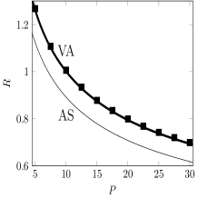
(a)

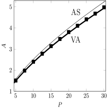
(b)

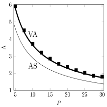
(c)

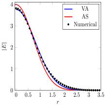
(d)

Figure 1: (color online) Comparison of both VA and AS approximations (solid lines) and numerical results (dots) for one dimensional ($D=1$) nonlocal solitons. Beam width $R$ (a), amplitude $A$ (b), and period of small oscillations $\Lambda$ (c), are shown as functions of power $P$. (d) Distribution of $|E|$ as a function of $r$ for power $P=20$. Other parameters are $d=40$, $z=100$.

Another useful approximation in AS approximation is based on the solution of Eq. (2) in the form of Eq. (11) when parameter $\Theta_{D}=A^{2}/\left(4D\right)=P_{D}/\left(4D\pi^{D/2}R^{D}\right)$ is independent of $z$. In contrast to Eq. (34), in which the condition $\Theta_{D}$ may depend on $z$, Eq. (32) for $R$ has an exact oscillatory solution Guo et al. (2004)

$$R=R_{*}\sqrt{\cos^{2}(\pi z/\Lambda)+\frac{P_{*}}{P_{D}}\sin^{2}(\pi z/\Lambda)},$$ (38)

from which the solutions for $C$ and $\psi$ immediately follow:

$$C=\frac{\pi}{\Lambda}\frac{\left(P_{*}/P_{D}-1\right)\sin(2\pi z/\Lambda)}{4\left(\cos^{2}(\pi z/\Lambda)+\left(P_{*}/P_{D}\right)\sin^{2}(\pi z/\Lambda)\right)},$$ (39)

$$\psi=-\arctan\left(\sqrt{P_{*}/P_{D}}\tan(\pi z/\Lambda)\right).$$ (40)

Here $R_{*}$ and $P_{*}$ are the width and the power of the AS solution, respectively. When $P_{D}=P_{*}$, one obtains stationary AS; otherwise, the approximate solution oscillates. The quantity $\Lambda=\Lambda_{AS}\sqrt{P_{*}/P_{D}}$ represents the period of harmonic oscillations around the equilibrium (soliton) state, while $\Lambda_{AS}$ is the period of small oscillations of the width perturbation:

$$\Lambda_{AS}=\pi R_{*}^{2}.$$ (41)

Thus, one obtains nice dependencies in closed form, but unfortunately of little practical value, in view of the large discrepancy with the VA and the numerical solution of the full problem, to be presented in the next section.

V Numerical Results

For numerical simulations of Eq. (1) we use finite difference time domain (FDTD) split-step method Aleksic et al. (2012). Equation (2) is solved by the tridiagonal matrix algorithm (TDMA). In our simulations we applied the same boundary conditions for both Eqs. (1,2):

$$\left(\frac{\partial E}{\partial r}\right)_{r=0}=0,\qquad E_{r=d}=0$$ (42)

and

$$\left(\frac{\partial\theta}{\partial r}\right)_{r=0}=0,\qquad\theta_{r=d}=0$$ (43)

The initial beam is the trial function given by Eq. (17), with parameters determined by VA approximation, Eqs. (25,26).

Figures (1,2,3) show analytical predictions of both approximations and numerical results for one, two, and three dimensions, respectively. The beam width $R$ of soliton solutions for AS approximation is $2^{D/(8-2D)}$ times smaller than the VA approximation at a same power, see panel (a) in Figs. (1,2,3). The corresponding stationary amplitudes in both approximations are presented in panel (b) of Figs.(1,2,3). Because $P_{D}=\pi^{D/2}A^{2}R^{D}$, the equilibrium amplitude $A$ in the AS approximation is $2^{D^{2}/(16-4D)}$ times greater than the one in the VA approximation at the same power. The period in the AS approximation is $2^{D/(4-D)}$ times less than that in the VA approximation at the same power, see panel (c) in Figs. (1,2,3). Panel (d) in Figs. (1,2,3) shows an example of the soliton shape predicted by VA and AS, as well as the numerical output after a long propagation distance.

Thus, the values of the beam parameters for AS are systematically off the values for the VA approximation. In all the cases the VA predictions are confirmed by numerical results. This confirms that, while AS approximation may represent a valuable aid for an easy understanding of highly nonlocal solitons, it is a poor approximation to the more exact approaches, such as the VA approximation, and to the numerical solution.

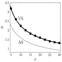
(a)

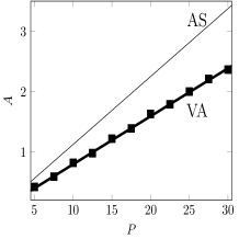
(b)

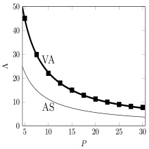
(c)

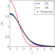
(d)

Figure 2: (color online) Same as Fig. (1), but for $D=2$. The only difference is in the propagation length, $z=10^{3}$.

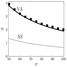
(a)

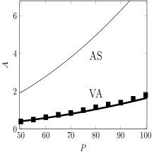
(b)

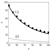
(c)

(d)

Figure 3: (color online) Same as Fig. (1), but for $D=3$. The propagation distance is now $z=10^{4}$ and $P=60$.

VI Conclusion

In conclusion, we have discussed the differences between the VA and AS approximate solutions to the propagation of solitons in highly nonlocal nonlinear media. The AS model provides a radical simplification of the problem and allows for an elegant description of solitons, but has a limited practical relevance, mainly because of the competition between the nonlocality and the finite size of the sample, which leads to systematic errors. The VA solution is not so simple, but it works very well in the limited region of large nonlocality. We have found that the AS approximation can differ up to eight times, when compared to the more realistic VA approximation and the numerical solution.