Low-energy theory of the Nambu-Goldstone modes of an ultracold ${}^{6}Li-$ ${}^{40}K$ mixture in an optical lattice

Abstract

A low-energy theory of the Nambu-Goldstone excitation spectrum and the corresponding speed of sound of an interacting Fermi mixture of Lithium-6 and Potassium-40 atoms in a two-dimensional optical lattice at finite temperatures with the Fulde-Ferrell order parameter has been formulated. It is assumed that the two-species interacting Fermi gas is described by the one-band Hubbard Hamiltonian with an attractive on-site interaction. The discussion is restricted to the BCS side of the Feshbach resonance where the Fermi atoms exhibit superfluidity. The quartic on-site interaction is decoupled via a Hubbard-Stratonovich transformation by introducing a four-component boson field which mediates the Hubbard interaction. A functional integral technique and a Legendre transform are used to give a systematic derivation of the Schwinger-Dyson equations for the generalized single-particle Green’s function and the Bethe-Salpeter equation for the two-particle Green’s function and the associated collective modes. The numerical solution of the Bethe-Salpeter equation in the generalized random phase approximation shows that there exist two distinct sound velocities in the long-wavelength limit. In addition to the long-wavelength mode (Goldstone mode), the two-species Fermi gas has a superfluid phase revealed by two rotonlike minima in the asymmetric collective-mode energy.

I Introduction

Optical lattices are formed by the interference of counter propagating laser beams. If the laser beams have equal frequencies, the gases of ultracold alkali atoms can be trapped in periodic potentials created by standing waves of laser light. Because of the Stark effect the ground-state alkali atoms couple to the electromagnetic field via an induced electric dipole moment. From theoretical point of view, the simplest approach to the trapped fermions is the tight-binding approximation, which requires sufficiently deep lattice potential. In the tight-binding limit, two alkali atoms of opposite pseudospins on the same site have an interaction energy $U$, while the probability to tunnel to a neighboring site is given by the hopping parameters. The hopping parameters as well as the interaction energy depend on the depth of the lattice potential and can be tuned by varying the intensity of the laser beams. We assume that the interacting fermions are in a sufficiently deep periodic lattice potential described by the Hubbard Hamiltonian. We restrict the discussion to the case of atoms confined to the lowest-energy band (single-band Hubbard model), with two possible states described by pseudospins $\sigma$. We consider different amounts of ${}^{6}Li$ and ${}^{40}K$ atoms in each state ($\sigma=\uparrow=Li$, $\sigma=\downarrow=K$) achieved by considering different chemical potentials $\mu_{\uparrow}$ and $\mu_{\downarrow}$. We assume that there are $M=M_{\uparrow}+M_{\downarrow}$ atoms distributed along $N$ sites, and the corresponding filling factors $f_{\uparrow,\downarrow}=M_{\uparrow,\downarrow}/N$ are smaller than unity. The Hubbard Hamiltonian is defined as follows:

$$H=-\sum_{<i,j>,\sigma}J_{\sigma}\psi^{\dagger}_{i,\sigma}\psi_{j,\sigma}-U\sum_{i}\widehat{n}_{i,\uparrow}\widehat{n}_{i,\downarrow}-\sum_{i,\sigma}\mu_{\sigma}\widehat{n}_{i,\sigma},$$ (1)

where $J_{\sigma}$ is the single electron hopping integral, and $\widehat{n}_{i,\sigma}=\psi^{\dagger}_{i,\sigma}\psi_{i,\sigma}$ is the density operator on site $i$. The Fermi operator $\psi^{\dagger}_{i,\sigma}$ ($\psi_{i,\sigma}$) creates (destroys) a fermion on the lattice site $i$ with pseudospin projection $\sigma$. The symbol $\sum_{<ij>}$ means sum over nearest-neighbor sites of the two-dimensional lattice. The first term in (1) is the usual kinetic energy term in a tight-binding approximation. All numerical calculations will be performed assuming that the hopping (tunneling) ratio $J_{Li}/J_{K}\approx 0.15$. In our notation the strength of the on-site interaction $U>0$ is positive, but the negative sign in front of the interaction corresponds to the Hubbard model with an attractive interaction. In the presence of an (effective) attractive interaction between the fermions, no matter how weak it is, the alkali atoms form bound pairs, also called the Cooper pairs. As a result, the system becomes unstable against the formation of a new many-body superfluid ground state. The superfluid ground state comes from the U(1) symmetry breaking and it is characterized by a nonzero order parameter, which in the population-balanced case is assumed to be a constant in space $\Delta_{0}$. Physically, it describes superfluid state of Cooper pairs with zero momentum. Superfluid state of Cooper pairs with nonzero momentum occurs in population-imbalanced case between a fermion with momentum $\textbf{k}+\textbf{q}$ and spin $\uparrow$ and a fermion with momentum $-\textbf{k}+\textbf{q}$, and spin $\downarrow$ . As a result, the pair momentum is $2\textbf{q}$. A finite pairing momentum implies a position-dependent phase of the order parameter, which in the Fulde-FerrellFF (FF) case varies as a single plane wave $\Delta(\textbf{r})=\Delta_{\textbf{q}}\exp\left(2\imath\textbf{q.r}\right)$, where $\Delta_{\textbf{q}}$ is a real quantity. The order parameter also can be a combination of two plane waves as in the case of the Larkin-OvchinnikovLO (LO) superfluid states. In both cases we are dealing with a spontaneous translational symmetry breaking and with an inhomogeneous superfluid state. When continuous and global symmetries are spontaneously broken the collective modes known as the Nambu-GoldstoneN ; G (NG) modes appear. From experimental point of view, the NG dispersion can be measured with unprecedented precision in systems of ultracold fermionic atoms on an optical lattice.SFexp1 ; SFexp2 ; SFexp3 ; SFexp4 ; SFexp5 ; SFexp6 ; SFexp7 ; SFexp8

Turning our attention to the theoretical description of the single-particle and collective-mode excitations of superfluid alkali atom Fermi gases in optical lattice potentials, we find that there have been impressive theoretical achievements. SF0 ; SF1 ; SF1a ; SF2 ; SF3 ; SF4 ; SF5 ; SF6 ; SF7 ; SF8 ; SF9 ; SF9a ; SF9b ; SF10 ; SF11 ; SF12 ; SF13 ; SF14 ; SF15 ; SF15a ; SF16 ; SF16a ; SF17 ; SF17a ; SF18 ; SF19 ; SF19a ; SF19b ; SF19c ; SF19d ; SF19e ; SF19g ; SF20 ; SF21 ; SF22 Generally speaking, the single-particle excitations manifest themselves as poles of the single-particle Green’s function, $G$; while the two-particle (collective) excitations could be related to the poles of the two-particle Green’s function, $K$. The poles of these Green’s functions are defined by the solutions of the Schwinger-Dyson (SD) equationSchwinger ; Dyson $G^{-1}=G^{(0)-1}-\Sigma$, and the Bethe-Salpeter (BS) equationBetheS $[K^{(0)-1}-I]\Psi=0$, respectively. Here, $G^{(0)}$ is the free single-particle propagator, $\Sigma$ is the fermion self-energy, $I$ is the BS kernel, and the two-particle free propagator $K^{(0)}=GG$ is a product of two fully dressed single-particle Green’s functions. Since the fermion self-energy depends on the two-particle Green’s function, the positions of both poles must to be obtained by solving the SD and BS equations self-consistently.

Instead of solving the SD and BS equations self-consistently, it is widely accepted that the single-particle dispersion can be obtained in the mean-field approximation or by solving the Bogoliubov-de Gennes (BdG) equations in a self-consistent fashion, while the generalized random phase approximation (GRPA) is the one that can provide the collective excitations in a weak-coupling regime. In the GRPA, the single-particle excitations are replaced with those obtained by diagonalizing the Hartree-Fock (HF) Hamiltonian; while the collective modes are obtained by solving the BS equation in which the single-particle Green’s functions are calculated in HF approximation, and the BS kernel is obtained by summing ladder and bubble diagrams.

There exist two different formulations of the GRPA that can be used to calculate the spectrum of the collective excitations of the Hubbard Hamiltonian (1). The first approach uses the Green’s function method,SF16a ; CGexc ; CG1 ; CCexc ; ZKexc ; Com ; ZGK ; ZK1 while the second one is based on the Anderson-Rickayzen equations.PA ; R ; BR ; SF17

The Green’s function approach has been used to obtain the collective excitations in the problems of the Bose-Einstein condensation (BEC) of excitons (or excitonic polaritons) in semiconductors,CGexc ; CCexc ; ZKexc and the BEC of Cooper pairs in s-wave layered superconductors. CG1 According to the Green’s function method, the collective modes manifest themselves as poles of the two-particle Green’s function, $K$, as well as the density and spin response functions. Both response functions can be expressed in terms of $K$, but it is very common to obtain the poles of the density response function by following the Baym and Kadanoff formalism,BK ; BK2 in which the density response function is defined in terms of functional derivatives of the density, with respect to the external fields.SF16a ; SF19

The second method that can be used to obtain the collective excitation spectrum of the Hubbard Hamiltonian starts from the Anderson-Rickayzen equations, which in the GRPA can be reduced to a set of three coupled equations, such that the collective-mode spectrum is obtained by solving a $3\times 3$ secular determinant.BR ; SF17

From theoretical point of view, the corresponding expressions for the Green’s functions cannot be evaluated exactly because the interaction part of the Hubbard Hamiltonian is quartic in the fermion fields. The simplest way to solve this problem is to apply the so-called mean-field decoupling of the quartic interaction. To go beyond the mean-field approximation, we apply the idea that we can transform the quartic term into quadratic form by making the Hubbard-Stratonovich transformation for the fermion operators. In contrast to the previous approaches, such that after performing the Hubbard-Stratonovich transformation the fermion degrees of freedom are integrated out; we decouple the quartic problem by introducing a model system which consists of a multi-component boson field $A_{\alpha}$ interacting with fermion fields $\psi^{\dagger}$ and $\psi$.

The functional-integral formulation of the Hubbard model requires the representation of the Hubbard interaction of (1) in terms of squares of one-body charge and spin operators. It is known that it may be possible to resolve the Hubbard interaction into quadratic forms of spin and electron number operators in an infinite number of ways.ZR If no approximations were made in evaluating the functional integrals, it would no matter which of the ways is chosen. When approximations are taken, the final result depends on a particular form chosen. Thus, one should check that the results obtained with the Hubbard-Stratonovich transformation are consistent with the results obtained with the canonical mean-field approximation. It can be seen that our approach to the Hubbard-Stratonovich transformation provides results consistent with the results obtained with the mean-field approximation, i.e. one can derive the mean-field gap equation using the collective-mode dispersion $\omega(Q)$ in the limit $Q\rightarrow 0$ and $\omega\rightarrow 0$.

There are three advantages of keeping both the fermion and the boson degrees of freedom. First, the approximation that is used to decouple the self-consistent relation between the fermion self-energy and the two-particle Green’s function automatically leads to conserving approximations because it relies on the fact that the BS kernel can be written as functional derivatives of the Fock $\Sigma^{F}$ and the Hartree $\Sigma^{H}$ self-energy $I=I_{d}+I_{exc}=\delta\Sigma^{F}/\delta G+\delta\Sigma^{H}/\delta G=\delta^{2}\Phi/\delta G\delta G$. As shown by Baym, BK2 any self-energy approximation is conserving whenever: (i) the self-energy can be written as the derivative of a functional $\Phi[G]$, i.e. $\Sigma=\delta\Phi[G]/\delta G$, and (ii) the SD equation for $G$ needs to be solved fully self-consistently for this form of the self-energy. Second, the collective excitations of the Hubbard model can be calculated in two different ways: as poles of the fermion Green’s function, $K$, and as poles of the boson Green’s function, $D$; or equivalently, as poles of the density and spin parts of the general response function, $\Pi$. Here, the boson Green’s function, $D$, is defined by the Dyson equation $D=D^{(0)}+D^{(0)}\Pi D^{(0)}$ where $D^{(0)}$ is the free boson propagator. Third, the action which describes the interactions in the Hubbard model is similar to the action $\psi^{\dagger}A\psi$ in quantum electrodynamics. This allows us to apply powerful field-theoretical methods, such as the method of Legendre transforms,DM to derive the SD and BS equations, as well as the vertex equation for the vertex function, $\Gamma$, and the Dyson equation for the boson Green’s function, $D$.

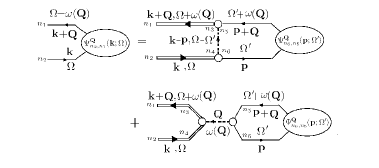
Figure 1: Diagrammatic representation of the Bethe-Salpeter equation (3) for the BS amplitude $\Psi^{\textbf{Q}}_{n_{2},n_{1}}(\textbf{k};\Omega)$. The single-particle Green’s function $G_{n_{2}n_{1}}(\textbf{k},\Omega)$ is represented by two solid lines, oriented in the direction of fermion propagation. The dashed lines represent the free boson propagator $D^{(0)}_{\alpha\beta}(\omega,\textbf{Q})$. At each of the bare vertices $\Gamma_{\alpha}^{(0)}(n_{1},n_{2})$ (represented by circles) the energy and momentum are conserved.

The basic assumption in the BS formalism is that the bound states of two fermions in the optical lattice at zero temperature are described by the BS wave functions (BS amplitudes). The BS amplitude determines the probability amplitude to find the first fermion at the site $i$ at the moment $t_{1}$ and the second fermion at the site $j$ at the moment $t_{2}$. The BS amplitude depends on the relative internal time $t_{1}-t_{2}$ and on the center-of-mass time $(t_{1}+t_{2})/2$:IZ

$$\begin{split}&\Phi^{\textbf{Q}}_{n_{2}n_{1}}(\textbf{r}_{i},\textbf{r}_{j};t_{1},t_{2})=\\ &\exp\left\{\imath\left[\textbf{Q.}(\textbf{r}_{i}+\textbf{r}_{j})/2-\omega(\textbf{Q})(t_{1}+t_{2})/2\right]\right\}\\ &\Psi^{\textbf{Q}}_{n_{2}n_{1}}(\textbf{r}_{i}-\textbf{r}_{j},t_{1}-t_{2}),\end{split}$$ (2)

where $\{n_{1},n_{2}\}$ are the corresponding quantum numbers, Q and $\omega(\textbf{Q})$ are the collective-mode momentum, and its dispersion, respectively. The Fourier transform $\Psi^{\textbf{Q}}_{n_{2},n_{1}}(\textbf{k};\Omega)$ of the BS amplitude

$$\Psi^{\textbf{Q}}_{n_{2}n_{1}}(\textbf{r},t)=\int\frac{d\Omega}{2\pi}\int\frac{d^{d}\textbf{k}}{(2\pi)^{d}}e^{\imath\left(\textbf{k}\textbf{.r}-\Omega t\right)}\Psi^{\textbf{Q}}_{n_{2},n_{1}}(\textbf{k};\Omega)$$

satisfies the BS equation, presented diagrammatically in Fig. 1. The direct interaction in the case of the Hubbard model is frequency independent; therefore the following BS equation for the equal-time BS amplitude $\Psi^{\textbf{Q}}_{n_{2},n_{1}}(\textbf{k})=\int\frac{d\Omega}{2\pi}\Psi^{\textbf{Q}}_{n_{2},n_{1}}(\textbf{k};\Omega)$ takes place:

$$\begin{split}&\Psi^{\textbf{Q}}_{n_{2},n_{1}}(\textbf{k})=\int\frac{d\Omega}{2\pi}G_{n_{1}n_{3}}\left(\textbf{k}+\textbf{Q},\Omega+\omega(\textbf{Q})\right)G_{n_{4}n_{2}}(\textbf{k},\Omega)\\ &\int\frac{d^{d}\textbf{p}}{(2\pi)^{d}}\left[I_{d}\left(\begin{array}[]{cc}n_{3}&n_{5}\\ n_{4}&n_{6}\\ \end{array}|\textbf{k}-\textbf{p}\right)+I_{exc}\left(\begin{array}[]{cc}n_{3}&n_{5}\\ n_{4}&n_{6}\\ \end{array}|\textbf{Q}\right)\right]\times\\ &\Psi^{\textbf{Q}}_{n_{6},n_{5}}(\textbf{p}).\end{split}$$ (3)

Here, $G_{n_{1}n_{2}}\left(\textbf{k},\Omega\right)$ is the Fourier transform of the single-particle dressed Green’s function, and $I_{d}$ and $I_{exc}$ are the direct and exchange parts of the BS kernel defined as functional derivatives of the Fock and the Hartree self-energies.

The superfluid states can be described in terms of the Namby-Gor’kov single-particle Green’s function which is a thermodynamic average of the $\widehat{T}_{u}$-ordered tensor product of the Nambu field operators

$$\widehat{\overline{\psi}}(y)=\left(\psi^{\dagger}_{\uparrow}(y)\psi_{\downarrow}(y)\right),\quad\widehat{\psi}(x)=\left(\begin{array}[]{c}\psi_{\uparrow}(x)\\ \psi^{\dagger}_{\downarrow}(x)\\ \end{array}\right).$$ (4)

As suggested by Maki,KM it is more convenient to use a spinor representation of the single-particle state by introducing the following four-component fermion fields

$$\begin{split}&\widehat{\Psi}(x)=\left(\begin{array}[]{c}\psi_{\uparrow}(x)\\ \psi_{\downarrow}(x)\\ \psi^{\dagger}_{\uparrow}(x)\\ \psi^{\dagger}_{\downarrow}(x)\\ \end{array}\right),\\ &\widehat{\Psi}^{\dagger}(y)=\left(\psi^{\dagger}_{\uparrow}(y)\psi^{\dagger}_{\downarrow}(y)\psi_{\uparrow}(y)\psi_{\downarrow}(y)\right).\end{split}$$ (5)

Here, we introduce composite variables $y=\{\textbf{r}_{i},u\}=\{i,u\}$ and $x=\{\textbf{r}_{i^{\prime}},u^{\prime}\}=\{i^{\prime},u^{\prime}\}$, where $\textbf{r}_{i},\textbf{r}_{i^{\prime}}$ are the lattice site vectors, and according to imaginary-time (Matsubara) formalism the variable $u,u^{\prime}$ range from $0$ to $\hbar\beta=\hbar/(k_{B}T)$. Throughout this paper we have assumed $\hbar=k_{B}=1$, the lattice constant $a=1$, and we use the summation-integration convention: that repeated variables are summed up or integrated over.

The field operators (4) allow us to define the Nambu-Gor’kov single-particle Green’s function:

$$\begin{split}&\widehat{G}(x_{1};y_{2})=-<\widehat{T}_{u}\left(\widehat{\psi}(x_{1})\otimes\widehat{\overline{\psi}}(y_{2})\right)>=\\ &-\left(\begin{array}[]{cc}<\widehat{T}_{u}\left(\psi_{\uparrow}(x_{1})\psi^{\dagger}_{\uparrow}(y_{2})\right)>&<\widehat{T}_{u}\left(\psi_{\uparrow}(x_{1})\psi_{\downarrow}(y_{2})\right)>\\ <\widehat{T}_{u}\left(\psi^{\dagger}_{\downarrow}(x_{1})\psi^{\dagger}_{\uparrow}(y_{2})\right)>&<\widehat{T}_{u}\left(\psi^{\dagger}_{\downarrow}(x_{1})\psi_{\downarrow}(y_{2})\right)>\\ \end{array}\right),\end{split}$$ (6)

and the generalized single-particle Green’s function which includes all possible thermodynamic averages:

$$\widehat{G}(x_{1};y_{2})=-<\widehat{T}_{u}\left(\widehat{\Psi}(x_{1})\otimes\widehat{\overline{\Psi}}(y_{2})\right)>$$

$$-\left(\begin{array}[]{cccc}<\widehat{T}_{u}\left(\psi_{\uparrow}(x_{1})\psi^{\dagger}_{\uparrow}(y_{2})\right)>&<\widehat{T}_{u}\left(\psi_{\uparrow}(x_{1})\psi^{\dagger}_{\downarrow}(y_{2})\right)>&<\widehat{T}_{u}\left(\psi_{\uparrow}(x_{1})\psi_{\uparrow}(y_{2})\right)>&<\widehat{T}_{u}\left(\psi_{\uparrow}(x_{1})\psi_{\downarrow}(y_{2})\right)>\\ <\widehat{T}_{u}\left(\psi_{\downarrow}(x_{1})\psi^{\dagger}_{\uparrow}(y_{2})\right)>&<\widehat{T}_{u}\left(\psi_{\downarrow}(x_{1})\psi^{\dagger}_{\downarrow}(y_{2})\right)>&<\widehat{T}_{u}\left(\psi_{\downarrow}(x_{1})\psi_{\uparrow}(y_{2})\right)>&<\widehat{T}_{u}\left(\psi_{\downarrow}(x_{1})\psi_{\downarrow}(y_{2})\right)>\\ <\widehat{T}_{u}\left(\psi^{\dagger}_{\uparrow}(x_{1})\psi^{\dagger}_{\uparrow}(y_{2})\right)>&<\widehat{T}_{u}\left(\psi^{\dagger}_{\uparrow}(x_{1})\psi^{\dagger}_{\downarrow}(y_{2})\right)>\par&<\widehat{T}_{u}\left(\psi^{\dagger}_{\uparrow}(x_{1})\psi_{\uparrow}(y_{2})\right)>&<\widehat{T}_{u}\left(\psi^{\dagger}_{\uparrow}(x_{1})\psi_{\downarrow}(y_{2})\right)>\\ <\widehat{T}_{u}\left(\psi^{\dagger}_{\downarrow}(x_{1})\psi^{\dagger}_{\uparrow}(y_{2})\right)>&<\widehat{T}_{u}\left(\psi^{\dagger}_{\downarrow}(x_{1})\psi^{\dagger}_{\downarrow}(y_{2})\right)>&<\widehat{T}_{u}\left(\psi^{\dagger}_{\downarrow}(x_{1})\psi_{\uparrow}(y_{2})\right)>&<\widehat{T}_{u}\left(\psi^{\dagger}_{\downarrow}(x_{1})\psi_{\downarrow}(y_{2})\right)>\\ \end{array}\right).$$ (11)

In the tight-binding approximation the BS equation (in the GRPA) can be reduced to a secular determinant, which determines the collective-mode dispersion. The Nambu-Gor’kov single-particle Green’s function (6) leads to the following $4\times 4$ secular determinant:SF18

$$Z_{4}=\left|\begin{array}[]{cccc}U^{-1}+\left(I_{\gamma,\gamma}-L_{\widetilde{\gamma},\widetilde{\gamma}}\right)&\left(J_{\gamma,l}-K_{m,\widetilde{\gamma}}\right)&\left(I_{\gamma,\widetilde{\gamma}}+L_{\gamma,\widetilde{\gamma}}\right)&\left(J_{\gamma,m}+K_{l,\widetilde{\gamma}}\right)\\ \left(J_{\gamma,l}-K_{m,\widetilde{\gamma}}\right)&U^{-1}+\left(I_{l,l}-L_{m,m}\right)&\left(J_{l,\widetilde{\gamma}}+K_{m,\gamma}\right)&\left(I_{l,m}+L_{l,m}\right)\\ \left(I_{\gamma,\widetilde{\gamma}}+L_{\gamma,\widetilde{\gamma}}\right)&\left(J_{l,\widetilde{\gamma}}+K_{m,\gamma}\right)&-U^{-1}+\left(I_{\widetilde{\gamma},\widetilde{\gamma}}-L_{\gamma,\gamma}\right)&\left(J_{\widetilde{\gamma},m}-K_{\gamma,l}\right)\\ \left(J_{\gamma,m}+K_{l,\widetilde{\gamma}}\right)&\left(I_{l,m}+L_{l,m}\right)&\left(J_{\widetilde{\gamma},m}-K_{\gamma,l}\right)&U^{-1}+\left(I_{m,m}-L_{l,l}\right)\end{array}\right|.$$ (12)

It is well known that when the generalized Green’s function (11) is used, the BS approach should provide a $16\times 16$ secular determinant. In what follows, we derive the corresponding $16\times 16$ secular determinant for a system of a ${}^{6}Li-$ ${}^{40}K$ mixture loaded in a two-dimensional optical lattice, and by means of it, we calculate numerically the collective-mode dispersion.

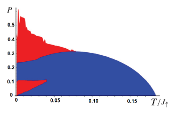
Figure 2: The phase diagrams of a ${}^{6}Li-$${}^{40}K$ mixture in a square lattice.SZ The interaction strength is $U=2J_{\uparrow}$. The polarization is defined as $P=(f_{K}-f_{Li})/f$, where the total filling is $f=0.5$ atoms/lattice site. Colors: Sarma states = blue (black), FF = red (dark grey), and normal gas = white.

The mean-field treatment of the FF and LO phases in a variety of systems, such as superconductors with Zeeman splitting, heavy-fermion superconductors,SC1 ; SC2 ; SC3 ; SC4 ; SC5 ; SC6 ; SC7 ; SC8 atomic Fermi gases with population imbalance loaded in optical latticesSF7 ; SF8 ; FG1 ; FG2 ; FG3 ; FG4 ; FG5 ; FG6 ; FG7 ; FG8 ; FG9 ; FG10 ; FG11 ; FG12 ; FG13 ; FG14 ; FG15 ; FG16 ; FG17 ; FG18 and harmonic traps, HTa and dense quark matter,DMa shows that the FF and LO states compete with a number of other states, such as the Sarma ($\textbf{q}=0$) states,Sa and the superfluid-normal separation phase (also known as the phase separation phase).FD1 ; FD2 ; FD3 ; FD4 It turns out that in some regions of momentum space the FF (or LO) phase provides the minimum of the mean-field expression of the Helmholtz free energy. The phase diagrams have been calculated for atomic Fermi gases in free space FDFS1 ; FDFS2 ; FDFS3 ; it was found that the parameter window for FF (or LO) states is extremely narrow. In contrast, a considerable parameter window for the existence of the FF phase has been found for population-imbalanced (but not mass-imbalanced) mixtures in an optical lattice. SF9 ; SF10 ; SF12 ; SF18 Phase diagrams for a ${}^{6}Li-$ ${}^{40}K$ mixture at zero temperature were obtained in Ref. [FDFS4, ], but the calculations were limited to the emergence of insulating phases during the evolution of superfluidity from the BCS to the BEC regime, and the competition between the FF and Sarma phases was ignored. The polarization versus temperature diagram,SZ presented in Fig. 2, shows that there are three phases: the Sarma phase, the FF phase, and the normal phase in which the Helmholtz free energy is minimized for gapless phase. The zero polarization line is the conventional Bardeen-Cooper-Schrieffer state. Contrary to the phase diagram of population-imbalanced ${}^{6}Li$ Fermi gas, where the phase separation appears for low polarizations, it was foundSZ the existence of a polarization window for the FF phase. This means that as soon as the system is polarized it goes into the FF phase if the temperature is low enough. This polarization window is larger for a majority of ${}^{40}K$ atoms compared to the majority of ${}^{6}Li$ atoms.

In what follows, we calculate the collective mode dispersion of the FF states numerically using the system parameters corresponding to a point in the above-mentioned polarization window for the FF phase: $f_{\uparrow}=0.225$, $f_{\downarrow}=0.275$, $U/J_{\uparrow}=2$ and $T/J_{\uparrow}=0.01$. The FF vector $\textbf{q}=(q_{x},q_{y})$, the gap and the chemical potentials in the mean-field approximation are defined by the solution of the mean-field equations (see Eqs. (39) in Sec. III): $\textbf{q}=(0.0489\pi/a,0)$, $\Delta_{\textbf{q}}/J_{\uparrow}=0.3668$, $\mu_{\uparrow}/J_{\uparrow}=2.0909$, and $\mu_{\downarrow}/J_{\uparrow}=0.5561$. For the Sarma state the corresponding mean-field values are as follows: $\Delta/J_{\uparrow}=0.3635$, $\mu_{\uparrow}/J_{\uparrow}=2.0466$, and $\mu_{\downarrow}/J_{\uparrow}=0.5918$. The FF phase is the most stable as it provides the minimum of the mean-field expression of the Helmholtz free energy (the ratio between the FF free energy and the Sarma free energy is about 0.9986).

The paper is organized as follows. In the next Section we apply the functional-integral formalism to derive equations for the single-particle excitations and for the two-particle collective modes. In Section III, we numerically solve the BS equation to obtain the Nambu-Goldstone excitation spectrum and the corresponding speed of sound of an interacting Fermi mixture of ${}^{6}Li-$ ${}^{40}K$ atoms in a two-dimensional optical lattice at finite temperatures with the Fulde-Ferrell order parameter. In the last Section we discuss the difference between the collective-mode dispersion, obtained by means of $4\times 4$ secular determinant, and obtained by the $16\times 16$ secular determinant.

II BETHE-SALPETER APPROACH TO THE COLLECTIVE MODES

II.1 The functional-integral technique

The Green’s functions in the functional-integral approach are defined by means of the so-called generating functional with sources for the boson and fermion fields. In our problem, the corresponding functional integrals cannot be evaluated exactly because the interaction part of the Hamiltonian (1) is quartic in the Grassmann fermion fields. However, we can transform the quartic terms to a quadratic form by introducing a model system which consists of a four-component boson field $A_{\alpha}(z)$ ($\alpha=1,2,3,4,\quad z=(\textbf{r}_{i},v),\quad 0\leq v\leq\beta)$ interacting with fermion fields $\widehat{\overline{\psi}}(y)=\widehat{\Psi}^{\dagger}(y)/\sqrt{2}$ and $\widehat{\psi}(x)=\widehat{\Psi}(x)/\sqrt{2}$. The action of this model system is assumed to be of the following form $S=S^{(F)}_{0}+S^{(B)}_{0}+S^{(F-B)}$, where:

$$S^{(F)}_{0}=\widehat{\overline{\psi}}(y)\widehat{G}^{(0)-1}(y;x)\widehat{\psi}(x),$$

$$S^{(B)}_{0}=\frac{1}{2}A_{\alpha}(z)D^{(0)-1}_{\alpha\beta}(z,z^{\prime})A_{\beta}(z^{\prime}),$$

$$S^{(F-B)}=\widehat{\overline{\psi}}(y)\widehat{\Gamma}^{(0)}_{\alpha}(y,x\mid z)\widehat{\psi}(x)A_{\alpha}(z).$$

The action $S^{(F)}_{0}$ describes the fermion part of the system. The generalized inverse Green’s function of free fermions $\widehat{G}^{(0)-1}(y;x)$ is given by the following diagonal matrix:

$$\begin{split}&\widehat{G}^{(0)-1}(y;x)=\\ &\sum_{\textbf{k},\omega_{m}}\exp\left[\imath\textbf{k.}(\textbf{r}_{i}-\textbf{r}_{i^{\prime}})-\omega_{m}(u-u^{\prime})\right]G_{n_{1}n_{2}}^{(0)-1}(\textbf{k},\imath\omega_{m}),\end{split}$$

where $G_{11}^{(0)-1}(\textbf{k},\imath\omega_{m})=-G_{33}^{(0)-1}(-\textbf{k},-\imath\omega_{m})$, and $-G_{22}^{(0)-1}(-\textbf{k},-\imath\omega_{m})=G_{44}^{(0)-1}(\textbf{k},\imath\omega_{m})$. The symbol $\sum_{\omega_{m}}$ is used to denote $\beta^{-1}\sum_{m}$ (for fermion fields $\omega_{m}=(2\pi/\beta)(m+1/2);m=0,\pm 1,\pm 2,...$). In the case of the FF states of a population-imbalanced Fermi gas, the non-interacting Green’s function is:

$$\widehat{G}^{(0)-1}(\textbf{k},\imath\omega_{m})=\left(\begin{array}[]{cccc}\imath\omega_{m}-\xi_{\uparrow}(\textbf{k})&0&0&0\\ 0&\imath\omega_{m}-\xi_{\downarrow}(\textbf{k})&0&0\\ 0&0&\imath\omega_{m}+\xi_{\uparrow}(\textbf{k})&0\\ 0&0&0&\imath\omega_{m}+\xi_{\downarrow}(\textbf{k})\end{array}\right),$$

where $\xi_{\uparrow,\downarrow}(\textbf{k})=2J_{\uparrow,\downarrow}(1-\cos k_{x})+2J_{\uparrow,\downarrow}(1-\cos k_{y})-\mu_{\uparrow,\downarrow}$.

The action $S^{(B)}_{0}$ describes the boson field which mediates the fermion-fermion on-site interaction in the Hubbard Hamiltonian. The bare boson propagator in $S^{(B)}_{0}$ is defined as:

$$\widehat{D}^{(0)}(z,z^{\prime})=\delta(v-v^{\prime})U\delta{j,j^{\prime}}\left(\begin{array}[]{cccc}0&1&0&0\\ 1&0&0&0\\ 0&0&0&0\\ 0&0&0&0\end{array}\right).$$

The Fourier transform of the boson propagator is given by

$$\widehat{D}^{(0)}(z,z^{\prime})=\frac{1}{N}\sum_{\textbf{k}}\sum_{\omega_{p}}e^{\left\{\imath\left[\textbf{k.}\left(\textbf{r}_{j}-\textbf{r}_{j^{\prime}}\right)-\omega_{p}\left(v-v^{\prime}\right)\right]\right\}}\widehat{D}^{(0)}(\textbf{k}),\widehat{D}^{(0)}(\textbf{k})=\left(\begin{array}[]{cccc}0&U&0&0\\ U&0&0&0\\ 0&0&0&0\\ 0&0&0&0\end{array}\right).$$ (13)

The interaction between the fermion and the boson fields is described by the action $S^{(F-B)}$. The bare vertex $\widehat{\Gamma}^{(0)}_{\alpha}(y_{1};x_{2}\mid z)=\widehat{\Gamma}^{(0)}_{\alpha}(i_{1},u_{1};i_{2},u_{2}\mid j,v)=\delta(u_{1}-u_{2})\delta(u_{1}-v)\delta_{i_{1}i_{2}}\delta_{i_{1}j}\widehat{\Gamma}^{(0)}(\alpha)$ is a $4\times 4$ matrix, where

$$\widehat{\Gamma}^{(0)}(\alpha)=\frac{1}{2}(\gamma_{0}+\alpha_{z})\delta_{\alpha 1}+\frac{1}{2}(\gamma_{0}-\alpha_{z})\delta_{\alpha 2}+\frac{1}{2}(\alpha_{x}+\imath\alpha_{y})\delta_{\alpha 3}+\frac{1}{2}(\alpha_{x}-\imath\alpha_{y})\delta_{\alpha 4}.$$ (14)

The Dirac matrix $\gamma_{0}$ and the matrices $\widehat{\alpha}_{i}$ are defined as (when a four-dimensional space is used,KM the electron spin operators $\sigma_{i}$ has to be replaced by $\widehat{\alpha}_{i}\gamma_{0}$):

$$\gamma_{0}=\left(\begin{array}[]{cccc}1&0&0&0\\ 0&1&0&0\\ 0&0&-1&0\\ 0&0&0&-1\\ \end{array}\right),\quad\widehat{\alpha}_{i}=\left(\begin{array}[]{cc}\sigma_{i}&0\\ 0&\sigma_{y}\sigma_{i}\sigma_{y}\\ \end{array}\right),i=x,y,z.$$

The relation between the Hubbard model and our model system can be demonstrated by applying the Hubbard-Stratonovich transformation for the fermion operators:

$$\int\mu[A]\exp\left[\widehat{\overline{\psi}}(y)\widehat{\Gamma}^{(0)}_{\alpha}(y;x|z)\widehat{\psi}(x)A_{\alpha}(z)\right]=\exp\left[-\frac{1}{2}\widehat{\overline{\psi}}(y)\widehat{\Gamma}^{(0)}_{\alpha}(y;x|z)\widehat{\psi}(x)D_{\alpha,\beta}^{(0)}(z,z^{\prime})\widehat{\overline{\psi}}(y^{\prime})\widehat{\Gamma}^{(0)}_{\beta}(y^{\prime};x^{\prime}|z^{\prime})\widehat{\psi}(x^{\prime})\right].$$ (15)

The functional measure $D\mu[A]$ is chosen to be:

$$\mu[A]=DAe^{-\frac{1}{2}A_{\alpha}(z)D_{\alpha,\beta}^{(0)-1}(z,z^{\prime})A_{\beta}(z^{\prime})},\int\mu[A]=1.$$

According to the field-theoretical approach, the expectation value of a general operator $\widehat{O}(u)$ can be expressed as a functional integral over the boson field $A$ and the Grassmann fermion fields $\widehat{\overline{\psi}}$ and $\widehat{\psi}$:

$$<\widehat{T}_{u}(\widehat{O}(u))>=\frac{1}{Z[J,M]}\int D\mu[\widehat{\overline{\psi}},\widehat{\psi},A]\widehat{O}(u)\exp\left[J_{\alpha}(z)A_{\alpha}(z)-M(\widehat{\overline{\psi}},\widehat{\psi})\right]|_{J=M=0},$$ (16)

where the symbol $<...>$ means that the thermodynamic average is made. The functional $Z[J,M]$ is defined by

$$Z[J,M]=\int D\mu[\widehat{\overline{\psi}},\widehat{\psi},A]\exp\left[J_{\alpha}(z)A_{\alpha}(z)-M(\widehat{\overline{\psi}},\widehat{\psi})\right],$$ (17)

where the functional measure $D\mu[\widehat{\overline{\psi}},\widehat{\psi},A]=DAD\widehat{\overline{\psi}}D\widehat{\psi}\exp\left(S\right)$ satisfies the condition $\int D\mu[\widehat{\overline{\psi}},\widehat{\psi},A]=1$. The quantity $J_{\alpha}(z)$ is the source of the boson field, while the sources $M_{ij}(y;x)$ of the fermion fields are included in the $M(\widehat{\overline{\psi}},\widehat{\psi})$ term :

$$M(\widehat{\overline{\psi}},\widehat{\psi})=\psi^{\dagger}_{\uparrow}(y)M_{11}(y;x)\psi_{\uparrow}(x)+\psi^{\dagger}_{\downarrow}(y)M_{21}(y;x)\psi_{\uparrow}(x)+\psi^{\dagger}_{\uparrow}(y)M_{12}(y;x)\psi_{\downarrow}(x)+\psi^{\dagger}_{\downarrow}(y)M_{22}(y;x)\psi_{\downarrow}(x)$$

$$+\psi_{\uparrow}(y)M_{31}(y;x)\psi_{\uparrow}(x)+\psi_{\downarrow}(y)M_{41}(y;x)\psi_{\uparrow}(x)+\psi_{\uparrow}(y)M_{32}(y;x)\psi_{\downarrow}(x)+\psi_{\downarrow}(y)M_{42}(y;x)\psi_{\downarrow}(x)$$

$$+\psi^{\dagger}_{\uparrow}(y)M_{13}(y;x)x)\psi^{\dagger}_{\uparrow}(x)+\psi^{\dagger}_{\downarrow}(y)M_{23}(y;x)\psi^{\dagger}_{\uparrow}(x)+\psi^{\dagger}_{\uparrow}(y)M_{14}(y;x)\psi^{\dagger}_{\downarrow}(x)+\psi^{\dagger}_{\downarrow}(y)M_{24}(y;x)\psi^{\dagger}_{\downarrow}(x)$$

$$+\psi_{\uparrow}(y)M_{33}(y;x)\psi^{\dagger}_{\uparrow}(x)+\psi_{\downarrow}(y)M_{43}(y;x)\psi^{\dagger}_{\uparrow}(x)+\psi_{\uparrow}(y)M_{34}(y;x)\psi^{\dagger}_{\downarrow}(x)+\psi_{\downarrow}(y)M_{44}(y;x)\psi^{\dagger}_{\downarrow}(x).$$ (18)

Here, we have introduced complex indices $1=\{n_{1},x_{1}\}$, and $2=\{n_{2},y_{2}\}$.

We shall now use a functional derivative $\delta/\delta M(2;1)$; depending on the spin degrees of freedom, there are sixteen possible derivatives. By means of the definition (16), one can express all Green’s functions in terms of the functional derivatives with respect to the corresponding sources of the generating functional of the connected Green’s functions $W[J,M]=\ln Z[J,M]$. Thus, we define the following Green’s and vertex functions which will be used to analyze the collective modes of our model:

The Boson Green’s function is $D_{\alpha\beta}(z,z^{\prime})$ is a $4\times 4$ matrix defined as $D_{\alpha\beta}(z,z^{\prime})=-\frac{\delta^{2}W}{\delta J_{\alpha}(z)\delta J_{\beta}(z^{\prime})}$.

The generalized single-fermion Green’s function $G_{n_{1}n_{2}}(x_{1};y_{2})$ is the matrix (11) whose elements are $G_{n_{1}n_{2}}(x_{1};y_{2})=-\delta W/\delta M_{n_{2}n_{1}}(y_{2};x_{1})$. Depending on the two spin degrees of freedom, $\uparrow$ and $\downarrow$, there exist eight ”normal” Green’s functions and eight ”anomalous” Green’s functions. We introduce Fourier transforms of the ”normal” $G_{\sigma_{1},\sigma_{2}}(\textbf{k},u_{1}-u_{2})=-<\widehat{T}_{u}(\psi_{\sigma_{1},\textbf{k}}(u_{1})\psi^{\dagger}_{\sigma_{2},\textbf{k}}(u_{2}))>$, and ”anomalous” $F_{\sigma_{1},\sigma_{2}}(\textbf{k},u_{1}-u_{2})=-<\widehat{T}_{u}(\psi_{\sigma_{1},\textbf{k}}(u_{1})\psi_{\sigma_{2},-\textbf{k}}(u_{2}))>$ one-particle Green’s functions, where $\{\sigma_{1},\sigma_{2}\}=\uparrow,\downarrow$. Here $\psi^{+}_{\uparrow,\textbf{k}}(u),\psi_{\uparrow,\textbf{k}}(u)$ and $\psi^{+}_{\downarrow,\textbf{k}}(u),\psi_{\downarrow,\textbf{k}}(u)$ are the creation-annihilation Heisenberg operators. The Fourier transform of the generalized single-particle Green’s function is given by

$$\widehat{G}(1;2)=\frac{1}{N}\sum_{\textbf{k}}\sum_{\omega_{m}}\exp\{\imath\left[\textbf{k.}\left(\textbf{r}_{i_{1}}-\textbf{r}_{i_{2}}\right)-\omega_{m}(u_{1}-u_{2})\right]\}\left(\begin{array}[]{cc}\widehat{G}(\textbf{k},\imath\omega_{m})&\widehat{F}(\textbf{k},\imath\omega_{m})\\ \widehat{F}^{\dagger}(\textbf{k},\imath\omega_{m})&-\widehat{G}(-\textbf{k},-\imath\omega_{m})\\ \end{array}\right).$$ (19)

Here, $\widehat{G}$ and $\widehat{F}$ are $2\times 2$ matrices whose elements are $G_{\sigma_{1},\sigma_{2}}$ and $F_{\sigma_{1},\sigma_{2}}$, respectively.

The two-particle Green’s function $K\left(\begin{array}[]{cc}n_{1},x_{1}&n_{3},y_{3}\\ n_{2},y_{2}&n_{4},x_{4}\\ \end{array}\right)$ is defined as

$$K\left(\begin{array}[]{cc}n_{1},x_{1}&n_{3},y_{3}\\ n_{2},y_{2}&n_{4},x_{4}\\ \end{array}\right)=K\left(\begin{array}[]{cc}1&3\\ 2&4\\ \end{array}\right)=\frac{\delta^{2}W}{\delta M_{n_{2}n_{1}}(y_{2};x_{1})\delta M_{n_{3}n_{4}}(y_{3};x_{4})}=-\frac{\delta G_{n_{1}n_{2}}(x_{1};y_{2})}{\delta M_{n_{3}n_{4}}(y_{3};x_{4})}.$$ (20)

This definition of $K$ allows us to conclude that if the approximation used for $G$ is chosen in accordance with the recipes proposed by Baym and Kadanoff,BK2 then $K$ is automatically conserving.

The vertex function $\widehat{\Gamma}_{\alpha}(2;1\mid z)$ for a given $\alpha$ is a $4\times 4$ matrix whose elements are:

$$\widehat{\Gamma}_{\alpha}(i_{2},u_{2};i_{1},u_{1}\mid v,j)_{n_{2}n_{1}}=-\frac{\delta G_{n_{2}n_{1}}^{-1}(i_{2},u_{2};i_{1},u_{1})}{\delta J_{\beta}(z^{\prime})}D^{-1}_{\beta\alpha}(z^{\prime},z).$$ (21)

II.2 Equations of the boson and fermion Green’s functions

It is well-known that the fermion self-energy (fermion mass operator) $\widehat{\Sigma}(1;2)$ can be defined by means of the so-called SD equations. They can be derived using the fact that the measure $D\mu[\overline{\psi},\psi,A]$ is invariant under the translations $\overline{\psi}\rightarrow\overline{\psi}+\delta\overline{\psi}$ and $A\rightarrow A+\delta A$:

$$D^{(0)-1}_{\alpha\beta}(z,z^{\prime})R_{\beta}(z^{\prime})+\frac{1}{2}Tr\left(\widehat{G}(1;2)\widehat{\Gamma}^{(0)}_{\alpha}(2;1\mid z)\right)+J_{\alpha}(z)=0,$$ (22)

$$\widehat{G}^{-1}(1;2)-\widehat{G}^{(0)-1}(1;2)+\widehat{\Sigma}(1;2)+\widehat{M}(1;2)=0,$$ (23)

where $R_{\alpha}(z)=\delta W/\delta J_{\alpha}(z)$ is the average boson field. The fermion self-energy $\widehat{\Sigma}$, is a $4\times 4$ matrix which can be written as a sum of Hartree $\widehat{\Sigma}^{H}$ and Fock $\widehat{\Sigma}^{F}$ parts. The Hartree part is a diagonal matrix whose elements are:

$$\Sigma^{H}(i_{1},u_{1};i_{2},u_{2})_{n_{1}n_{2}}=\frac{1}{2}\widehat{\Gamma}_{\alpha}^{(0)}(i_{1},u_{1};i_{2},u_{2}|j,v)_{n_{1}n_{2}}D^{(0)}_{\alpha\beta}(j,v;j^{\prime},v^{\prime})\widehat{\Gamma}_{\beta}^{(0)}(i_{3},u_{3};i_{4},u_{4}|j^{\prime},v^{\prime})_{n_{3}n_{4}}G_{n_{4}n_{3}}(i_{4},u_{4};i_{3},u_{3}).$$ (24)

The Fock part of the fermion self-energy is given by:

$$\begin{split}&\Sigma^{F}(i_{1},u_{1};i_{2},u_{2})_{n_{1}n_{2}}=-\widehat{\Gamma}_{\alpha}^{(0)}(i_{1},u_{1};i_{6},u_{6}|j,v)_{n_{1}n_{6}}D^{(0)}_{\alpha\beta}(j,v;j^{\prime},v^{\prime})\widehat{\Gamma}_{\beta}^{(0)}(i_{4},u_{4};i_{5},u_{5}|j^{\prime},v^{\prime})_{n_{4}n_{5}}\times\\ &K\left(\begin{array}[]{cc}n_{5},i_{5},u_{5}&n_{3},i_{3},u_{3}\\ n_{4},i_{4},u_{4}&n_{6},i_{6},u_{6}\\ \end{array}\right)G^{-1}_{n_{3}n_{2}}(i_{3},u_{3};i_{2},u_{2}).\end{split}$$ (25)

The Fock part of the fermion self-energy depends on the two-particle Green’s function $K$; therefore the SD equations and the BS equation for $K$ have to be solved self-consistently.

Our approach to the Hubbard model allows us to obtain exact equations of the Green’s functions by using the field-theoretical technique. We now wish to return to our statement that the Green’s functions are the thermodynamic average of the $\widehat{T}_{u}$-ordered products of field operators. The standard procedure for calculating the Green’s functions, is to apply Wick’s theorem. This enables us to evaluate the $\widehat{T}_{u}$-ordered products of field operators as a perturbation expansion involving only wholly contracted field operators. These expansions can be summed formally to yield different equations of Green’s functions. The main disadvantage of this procedure is that the validity of the equations must be verified diagram by diagram. For this reason we will use the method of Legendre transforms of the generating functional for connected Green’s functions.DM By applying the same steps as in Ref. [ZKexc, ] we obtain the BS equation of the two-particle Green’s function, the Dyson equation of the boson Green’s function, and the vertex equation:

$$K^{-1}\left(\begin{array}[]{cc}n_{2},i_{2},u_{2}&n_{3},i_{3},u_{3}\\ n_{1},i_{1},u_{1}&n_{4},i_{4},u_{4}\\ \end{array}\right)=K^{(0)-1}\left(\begin{array}[]{cc}n_{2},i_{2},u_{2}&n_{3},i_{3},u_{3}\\ n_{1},i_{1},u_{1}&n_{4},i_{4},u_{4}\\ \end{array}\right)-I\left(\begin{array}[]{cc}n_{2},i_{2},u_{2}&n_{3},i_{3},u_{3}\\ n_{1},i_{1},u_{1}&n_{4},i_{4},u_{4}\\ \end{array}\right),$$ (26)

$$D_{\alpha\beta}(z,z^{\prime})=D^{(0)}_{\alpha\beta}(z,z^{\prime})+D^{(0)}_{\alpha\gamma}(z,z^{\prime\prime})\Pi_{\gamma\delta}(z^{\prime\prime},z^{\prime\prime\prime})D^{(0)}_{\delta\beta}(z,z^{\prime}),$$ (27)

$$\begin{split}&\widehat{\Gamma}_{\alpha}(i_{2},u_{2};i_{1},u_{1}\mid z)_{n_{2}n_{1}}=\widehat{\Gamma}^{(0)}_{\alpha}(i_{2},u_{2};i_{1},u_{1}\mid z)_{n_{2}n_{1}}+I\left(\begin{array}[]{cc}n_{2},i_{2},u_{2}&n_{3},i_{3},u_{3}\\ n_{1},i_{1},u_{1}&n_{4},i_{4},u_{4}\\ \end{array}\right)\times\\ &K^{(0)}\left(\begin{array}[]{cc}n_{3},i_{3},u_{3}&n_{6},i_{6},u_{6}\\ n_{4},i_{4},u_{4}&n_{5},i_{5},u_{5}\\ \end{array}\right)\widehat{\Gamma}_{\alpha}(i_{6},u_{6};i_{5},u_{5}\mid z)_{n_{6}n_{5}}.\end{split}$$ (28)

Here,

$$K^{(0)}\left(\begin{array}[]{cc}n_{2},i_{2},u_{2}&n_{3},i_{3},u_{3}\\ n_{1},i_{1},u_{1}&n_{4},i_{4},u_{4}\\ \end{array}\right)=G_{n_{2}n_{3}}(i_{2},u_{3};i_{2},u_{2})G_{n_{4}n_{1}}(i_{4},u_{4};i_{1},u_{1})$$

is the two-particle free propagator constructed from a pair of fully dressed generalized single-particle Green’s functions. The kernel $I=\delta\Sigma/\delta G$ of the BS equation can be expressed as a functional derivative of the fermion self-energy $\widehat{\Sigma}$. Since $\widehat{\Sigma}=\widehat{\Sigma}^{H}+\widehat{\Sigma}^{F}$, the BS kernel $I=I_{exc}+I_{d}$ is a sum of functional derivatives of the Hartree $\Sigma^{H}$ and Fock $\Sigma^{F}$ contributions to the self-energy:

$$I_{exc}\left(\begin{array}[]{cc}n_{2},i_{2},u_{2}&n_{3},i_{3},u_{3}\\ n_{1},i_{1},u_{1}&n_{4},i_{4},u_{4}\\ \end{array}\right)=\frac{\delta\Sigma^{H}(i_{2},u_{2};i_{1},u_{1})_{n_{2}n_{1}}}{\delta G_{n_{3}n_{4}}(i_{3},u_{3};i_{4},u_{4})},\quad I_{d}\left(\begin{array}[]{cc}n_{2},i_{2},u_{2}&n_{3},i_{3},u_{3}\\ n_{1},i_{1},u_{1}&n_{4},i_{4},u_{4}\\ \end{array}\right)=\frac{\delta\Sigma^{F}(i_{2},u_{2};i_{1},u_{1})_{n_{2}n_{1}}}{\delta G_{n_{3}n_{4}}(i_{3},u_{3};i_{4},u_{4})}.$$ (29)

The general response function $\Pi$ in the Dyson equation (27) is defined as

$$\Pi_{\alpha\beta}(z,z^{\prime})=\widehat{\Gamma}^{(0)}_{\alpha}(i_{1},u_{1};i_{2},u_{2}\mid z)_{n_{1}n_{2}}K\left(\begin{array}[]{cc}n_{2},i_{2},u_{2}&n_{3},i_{3},u_{3}\\ n_{1},i_{1},u_{1}&n_{4},i_{4},u_{4}\\ \end{array}\right)\widehat{\Gamma}^{(0)}_{\beta}(i_{3},u_{3},i_{4},u_{4}\mid z^{\prime})_{n_{3}n_{4}}.$$ (30)

The functions $D$, $K$ and $\widehat{\Gamma}$ are related by the identity:

$$\begin{split}&K^{(0)}\left(\begin{array}[]{cc}n_{2},i_{2},u_{2}&n_{3},i_{3},u_{3}\\ n_{1},i_{1},u_{1}&n_{4},i_{4},u_{4}\\ \end{array}\right)\widehat{\Gamma}_{\beta}(i_{4},u_{4};i_{3},u_{3}\mid z^{\prime})_{n_{4}n_{3}}D_{\beta\alpha}(z^{\prime},z)\\ &=K\left(\begin{array}[]{cc}n_{2},i_{2},u_{2}&n_{3},i_{3},u_{3}\\ n_{1},i_{1},u_{1}&n_{4},i_{4},u_{4}\\ \end{array}\right)\widehat{\Gamma}^{(0)}_{\beta}(i_{4},u_{4};i_{3},u_{3}\mid z^{\prime})_{n_{4}n_{3}}D^{(0)}_{\beta\alpha}(z^{\prime},z),\end{split}$$ (31)

By introducing the boson proper self-energy $P^{-1}_{\alpha\beta}(z,z^{\prime})=\Pi^{-1}_{\alpha\beta}(z,z^{\prime})+D^{(0)}_{\alpha\beta}(z,z^{\prime})$ one can rewrite the Dyson equation (27) for the boson Green’s function as:

$$D^{-1}_{\alpha\beta}(z,z^{\prime})=D^{(0)-1}_{\alpha\beta}(z,z^{\prime})-P_{\alpha\beta}(z,z^{\prime}).$$ (32)

The proper self-energy and the vertex function $\widehat{\Gamma}$ are related by the following equation:

$$\begin{split}&P_{\alpha\beta}(z,z^{\prime})=\frac{1}{2}Tr\left[\widehat{\Gamma}_{\alpha}^{(0)}(y_{1},x_{2}|z)\widehat{G}(x_{2},y_{3})\widehat{\Gamma}_{\beta}(y_{3},x_{4}|z^{\prime})\widehat{G}(x_{4},y_{1})\right]\\ &=\frac{1}{2}\widehat{\Gamma}^{(0)}_{\alpha}(i_{1},u_{1};i_{2},u_{2}\mid z)_{n_{1}n_{2}}G_{n_{2}n_{3}}(i_{2},u_{2};i_{3},u_{3})\widehat{\Gamma}_{\beta}(i_{3},u_{3};i_{4},u_{4}\mid z^{\prime})_{n_{3}n_{4}}G_{n_{4}n_{1}}(i_{4},u_{4};i_{1},u_{1}).\end{split}$$ (33)

It is also possible to express the proper self-energy in terms of the two-particle Green’s function $\widetilde{K}$ which satisfies the BS equation $\widetilde{K}^{-1}=K^{(0)-1}-I_{d}$, but its kernel $I_{d}=\delta\Sigma^{F}/\delta G$ includes only diagrams that represent the direct interactions:

$$\begin{split}&P_{\alpha\beta}(z,z^{\prime})=\widehat{\Gamma}^{(0)}_{\alpha}(i_{1},u_{1};i_{2},u_{2}\mid z)_{n_{1}n_{2}}\widetilde{K}\left(\begin{array}[]{cc}n_{2},i_{2},u_{2}&n_{3},i_{3},u_{3}\\ n_{1},i_{1},u_{1}&n_{4},i_{4},u_{4}\\ \end{array}\right)\widehat{\Gamma}^{(0)}_{\beta}(i_{3},u_{3};i_{4},u_{4}\mid z^{\prime})_{n_{3}n_{4}}\\ &=\widehat{\Gamma}^{(0)}_{n_{1}n_{2}}(\alpha)\widetilde{K}\left(\begin{array}[]{cc}n_{2},\textbf{r}_{j},v&n_{3},\textbf{r}_{j^{\prime}},v^{\prime}\\ n_{1},\textbf{r}_{j},v&n_{4},\textbf{r}_{j^{\prime}},v^{\prime}\\ \end{array}\right)\widehat{\Gamma}^{(0)}_{n_{3}n_{4}}(\beta).\end{split}$$ (34)

One can obtain the spectrum of the collective excitations as poles of the boson Green’s function by solving the Dyson equation (32), but one has first to deal with the BS equation for the function $\widetilde{K}$. In other words, this method involves two steps. For this reason, it is easy to obtain the collective modes by locating the poles of the two-particle Green’s function $K$ using the solutions of the corresponding BS equation.

II.3 Mean-field approximation for the generalized single-particle Green’s functions

As we have already mentioned, the BS equation and the SD equations have to be solved self-consistently. In what follows, we use an approximation which allows us to decouple the above-mentioned equations and to obtain a linearized integral equation for the Fock term. To apply this approximation we first use Eq. (31) to rewrite the Fock term as

$$\Sigma^{F}(i_{1},u_{1};i_{2},u_{2})_{n_{1}n_{2}}=-\widehat{\Gamma}_{\alpha}^{(0)}(i_{1},u_{1};i_{3},u_{3}|j,v)_{n_{1}n_{3}}D_{\alpha\beta}(j,v;j^{\prime},v^{\prime})G_{n_{3}n_{4}}(i_{3},u_{3};i_{4},u_{4})\widehat{\Gamma}_{\beta}(i_{4},u_{4};i_{2},u_{2}|j^{\prime},v^{\prime})_{n_{4}n_{2}},$$ (35)

and after that we replace $D$ and $\widehat{\Gamma}$ in (35) by the free boson propagator $D^{(0)}$ and by the bare vertex $\widehat{\Gamma}^{(0)}$, respectively. In this approximation the Fock term assumes the form:

$$\begin{split}&\Sigma_{0}^{F}(i_{1},u_{1};i_{2},u_{2})_{n_{1}n_{2}}=-\widehat{\Gamma}_{\alpha}^{(0)}(i_{1},u_{1};i_{3},u_{3}|j,v)_{n_{1}n_{3}}D^{(0)}_{\alpha\beta}(j,v;j^{\prime},v^{\prime})\widehat{\Gamma}_{\beta}^{(0)}(i_{4},u_{4};i_{2},u_{2}|j^{\prime},v^{\prime}))_{n_{4}n_{2}}G_{n_{3}n_{4}}(i_{3},u_{3};i_{4},u_{4})=\\ &-U\delta_{i_{1},i_{2}}\delta(u_{1}-u_{2})\left(\begin{array}[]{cccc}0&G_{12}(1;2)&0&-G_{14}(1;2)\\ G_{21}(1;2)&0&-G_{23}(1;2)&0\\ 0&-G_{32}(1;2)&0&G_{34}(1;2)\\ -G_{41}(1;2)&0&G_{43}(1;2)&0\\ \end{array}\right).\end{split}$$ (36)

The total self-energy is $\widehat{\Sigma}(i_{1},u_{1};i_{2},u_{2})=\widehat{\Sigma}^{H}(i_{1},u_{1};i_{2},u_{2})+\widehat{\Sigma}^{F}(i_{1},u_{1};i_{2},u_{2})$, where

$$\begin{split}&\widehat{\Sigma}^{H}(i_{1},u_{1};i_{2},u_{2})=\\ &\frac{U}{2}\delta_{i_{1},i_{2}}\delta(u_{1}-u_{2})\left(\begin{array}[]{cccc}G_{22}(1;2)-G_{44}(1;2)&0&0&0\\ 0&G_{11}(1;2)-G_{33}(1;2)&0&0\\ 0&0&G_{44}(1;2)-G_{22}(1;2)&0\\ 0&0&0)&G_{33}(1;2)-G_{11}(1;2)\\ \end{array}\right)\end{split}$$ (37)

The contributions to $\Sigma(i_{1},u_{1};i_{2},u_{2})$, due to the elements on the major diagonal of the above matrices, will be included into the chemical potential. To obtain an analytical expression for the generalized single-particle Green’s function, we assume two more approximations. First, since the experimentally relevant magnetic fields are not strong enough to cause spin flips, we shall neglect $G_{12}=G_{21}=G_{34}=G_{43}=0$. Second, we neglect the frequency dependence of the Fourier transform of the Fock part of the fermion self-energy. Thus, the Dyson equation for the generalized single-particle Green’s function becomes:

$$\widehat{G}^{-1}(1;2)=\left(\begin{array}[]{cccc}G^{(0)-1}_{11}(1;2)&0&0&-\Delta e^{\imath 2\textbf{q.r}_{i_{1}}}\delta(\textbf{r}_{i_{1}}-\textbf{r}_{i_{2}})\\ 0&G^{(0)-1}_{22}(1;2)&\Delta e^{\imath 2\textbf{q.r}_{i_{1}}}\delta(\textbf{r}_{i_{1}}-\textbf{r}_{i_{2}})&0\\ 0&\Delta e^{-\imath 2\textbf{q.r}_{i_{1}}}\delta(\textbf{r}_{i_{1}}-\textbf{r}_{i_{2}})&G^{(0)-1}_{33}(1;2)&0\\ -\Delta e^{-\imath 2\textbf{q.r}_{i_{1}}}\delta(\textbf{r}_{i_{1}}-\textbf{r}_{i_{2}})&0&0&G^{(0)-1}_{44}(1;2)\\ \end{array}\right)$$

We can eliminate the phase factors $e^{\imath 2\textbf{q.r}_{i_{1}}}$ by performing the unitary transformation between the old generalized single-particle Green’s function $\widehat{G}$ and the new one $\widehat{\widetilde{G}}$, i.e. $\widehat{\widetilde{G}}(1;2)=U(1).\widehat{G}(1;2).U^{\dagger}(2)$, where the corresponding matrix is as follows

$$U(1)=\left(\begin{array}[]{cccc}e^{-\imath\textbf{q.r}_{i_{1}}}&0&0&0\\ 0&-e^{-\imath\textbf{q.r}_{i_{1}}}&0&0\\ 0&0&-e^{\imath\textbf{q.r}_{i_{1}}}&0\\ 0&0&0&e^{\imath\textbf{q.r}_{i_{1}}}\\ \end{array}\right).$$

After performing this unitary transformation, the Green’s function $\widehat{\widetilde{G}}(1;2)$ become functions of $\widehat{\widetilde{G}}(\textbf{r}_{i_{1}}-\textbf{r}_{i_{2}};u_{1}-u_{2})$, and the corresponding Fourier transform is:

$$\begin{split}&\widehat{\widetilde{G}}(1;2)=\sum_{\textbf{k},\omega_{m}}\exp\left[\imath(\textbf{k.}(\textbf{r}_{i_{1}}-\textbf{r}_{i_{2}})-\omega_{m}(u_{1}-u_{2})\right]\times\\ &\left(\begin{array}[]{cccc}\widetilde{G}_{11}(\textbf{k},\imath\omega_{m})&0&0&\widetilde{G}_{14}(\textbf{k},\imath\omega_{m})\\ 0&\widetilde{G}_{22}(\textbf{k},\imath\omega_{m})&\widetilde{G}_{23}(\textbf{k},\imath\omega_{m})&0\\ 0&\widetilde{G}_{32}(\textbf{k},\imath\omega_{m})&\widetilde{G}_{33}(\textbf{k},\imath\omega_{m})&0\\ \widetilde{G}_{41}(\textbf{k},\imath\omega_{m})&0&0&\widetilde{G}_{44}(\textbf{k},\imath\omega_{m})\\ \end{array}\right)\end{split}$$ (38)

III Collective modes of ${}^{6}Li-$ ${}^{40}K$ mixture

The FF superfluid state is expected to occur on the BCS side of the Feshbach resonance, where the effective attractive interaction between fermion atoms leads to BCS type pairing. In the case when the order parameter is assumed to vary as a single plane wave, we have a broken translational invariance, and as a result, the normal and anomalous Green’s functions have phase factors associated with the FF quasimomentum q, which can be eliminated using the previously mentioned unitary transformation.

In the mean filed approximation, the FF vector q, as well as the chemical potentials $\mu_{\uparrow}$ and $\mu_{\downarrow}$, and the gap $\Delta_{\textbf{q}}$ are defined by the solutions of following set of four equations (the number equations, the gap equation and the q-equation):SF18

$$\begin{split}&f_{\uparrow}=\frac{1}{N}\sum_{\textbf{k}}\left[u_{\textbf{q}}^{2}(\textbf{k})f(\omega_{+}(\textbf{k},\textbf{q}))+v_{\textbf{q}}^{2}(\textbf{k})f(-\omega_{-}(\textbf{k},\textbf{q}))\right],\quad f_{\downarrow}=\frac{1}{N}\sum_{\textbf{k}}\left[u_{\textbf{q}}^{2}(\textbf{k})f(\omega_{-}(\textbf{k},\textbf{q}))+v_{\textbf{q}}^{2}(\textbf{k})f(-\omega_{+}(\textbf{k},\textbf{q}))\right],\\ &1=\frac{U}{N}\sum_{\textbf{k}}\frac{1-f(\omega_{-}(\textbf{k},\textbf{q}))-f(\omega_{+}(\textbf{k},\textbf{q}))}{2E_{\textbf{q}}(\textbf{k})},\\ &0=\frac{1}{N}\sum_{\textbf{k}}\left\{\frac{\partial\eta_{\textbf{q}}(\textbf{k})}{\partial q_{x}}\left[f(\omega_{+}(\textbf{k},\textbf{q}))-f(\omega_{-}(\textbf{k},\textbf{q}))\right]+\frac{\partial\chi_{\textbf{q}}(\textbf{k})}{\partial q_{x}}\left[1-\frac{\chi_{\textbf{q}}(\textbf{k})}{E_{\textbf{q}}(\textbf{k})}\left[1-f(\omega_{+}(\textbf{k},\textbf{q}))-f(\omega_{-}(\textbf{k},\textbf{q}))\right]\right]\right\},\\ &\chi_{\textbf{q}}(\textbf{k})=\frac{1}{2}\left[\xi_{\uparrow}(\textbf{q}+\textbf{k})+\xi_{\downarrow}(\textbf{q}-\textbf{k})\right],\quad\eta_{\textbf{q}}(\textbf{k})=\frac{1}{2}\left[\xi_{\uparrow}(\textbf{q}+\textbf{k})-\xi_{\downarrow}(\textbf{q}-\textbf{k})\right],\quad\omega_{\pm}(\textbf{k},\textbf{q})=E_{\textbf{q}}(\textbf{k})\pm\eta_{\textbf{q}}(\textbf{k}),\\ &u_{\textbf{q}}^{2}(\textbf{k})=\frac{1}{2}\left[1+\frac{\chi_{\textbf{q}}(\textbf{k})}{E_{\textbf{q}}(\textbf{k})}\right],v_{\textbf{q}}^{2}(\textbf{k})=\frac{1}{2}\left[1-\frac{\chi_{\textbf{q}}(\textbf{k})}{E_{\textbf{q}}(\textbf{k})}\right],\quad E_{\textbf{q}}(\textbf{k})=\sqrt{\chi_{\textbf{q}}^{2}(\textbf{k})+\Delta_{\textbf{q}}^{2}},\end{split}$$ (39)

The Fourier transform of the generalized single-particle Green’s function in the mean field approximation is as follows:

$$\begin{split}&\widehat{\widetilde{G}}^{\textbf{q}}(\textbf{k},\imath\omega_{m})=\left(\begin{array}[]{cccc}\frac{\imath\omega_{m}+\xi_{\downarrow}(\textbf{q}-\textbf{k})}{A(\textbf{q},\textbf{k},\imath\omega_{m})}&0&0&\frac{\Delta_{\textbf{q}}}{A(\textbf{q},\textbf{k},\imath\omega_{m})}\\ 0&\frac{\imath\omega_{m}+\xi_{\uparrow}(\textbf{q}-\textbf{k})}{B(\textbf{q},\textbf{k},\imath\omega_{m})}&-\frac{\Delta_{\textbf{q}}}{B(\textbf{q},\textbf{k},\imath\omega_{m})}&0\\ 0&-\frac{\Delta_{\textbf{q}}}{B(\textbf{q},\textbf{k},\imath\omega_{m})}&\frac{\imath\omega_{m}-\xi_{\downarrow}(\textbf{q}+\textbf{k})}{B(\textbf{q},\textbf{k},\imath\omega_{m})}&0\\ \frac{\Delta_{\textbf{q}}}{A(\textbf{q},\textbf{k},\imath\omega_{m})}&0&0&\frac{\imath\omega_{m}-\xi_{\uparrow}(\textbf{q}+\textbf{k})}{A(\textbf{q},\textbf{k},\imath\omega_{m})}\\ \end{array}\right),\\ &A(\textbf{q},\textbf{k},\imath\omega_{m})=\left(\imath\omega_{m}-\xi_{\uparrow}(\textbf{q}+\textbf{k})\right)\left(\imath\omega_{m}+\xi_{\downarrow}(\textbf{q}-\textbf{k})\right)-\Delta_{\textbf{q}}^{2},\\ &B(\textbf{q},\textbf{k},\imath\omega_{m})=\left(\imath\omega_{m}-\xi_{\downarrow}(\textbf{q}+\textbf{k})\right)\left(\imath\omega_{m}+\xi_{\uparrow}(\textbf{q}-\textbf{k})\right)-\Delta_{\textbf{q}}^{2}.\end{split}$$ (40)

The spectrum of the collective modes will be obtained by solving the BS equation in the GRPA. As we have already mentioned, the kernel of the BS equation is a sum of the direct $I_{d}=\delta\Sigma^{F}/\delta G$ and exchange $I_{exc}=\delta\Sigma^{H}/\delta G$ interactions, written as derivatives of the Fock (36) and the Hartree (37) parts of the self-energy. Thus, in the GRPA the corresponding equation for the BS amplitude $\Psi^{\textbf{Q}}_{n_{2},n_{1}}=\int\frac{d\Omega}{2\pi}\int\frac{d^{d}\textbf{k}}{(2\pi)^{d}}\Psi^{\textbf{Q}}_{n_{2},n_{1}}(\textbf{k};\Omega)$ can be obtained from Eq. (3) by performing integration over the momentum vectors:

$$\Psi^{\textbf{Q}}_{n_{2}n_{1}}=K^{(0)}\left(\begin{array}[]{cc}n_{1}&n_{3}\\ n_{2}&n_{4}\\ \end{array}|\omega(\textbf{Q})\right)\left[I_{d}\left(\begin{array}[]{cc}n_{3}&n_{5}\\ n_{4}&n_{6}\\ \end{array}\right)+I_{exc}\left(\begin{array}[]{cc}n_{3}&n_{5}\\ n_{4}&n_{6}\\ \end{array}\right)\right]\Psi^{\textbf{Q}}_{n_{6},n_{5}},$$ (41)

where the two-particle propagator $K^{(0)}$ and the direct and exchange interactions are defined as follows:

$$\begin{split}&K^{(0)}\left(\begin{array}[]{cc}n_{1}&n_{3}\\ n_{2}&n_{4}\\ \end{array}|\omega(\textbf{Q})\right)\equiv K_{n_{1}n_{3}n_{4}n_{2}}=\int\frac{d\Omega}{2\pi}\int\frac{d^{d}\textbf{k}}{(2\pi)^{d}}\widetilde{G}_{n_{1}n_{3}}\left(\textbf{k}+\textbf{Q},\Omega+\omega(\textbf{Q})\right)\widetilde{G}_{n_{4}n_{2}}(\textbf{k},\Omega),\\ &I_{d}\left(\begin{array}[]{cc}n_{1}&n_{3}\\ n_{2}&n_{4}\\ \end{array}\right)=-\Gamma^{(0)}_{\alpha}(n_{1},n_{3})D^{(0)}_{\alpha\beta}\Gamma^{(0)}_{\beta}(n_{4},n_{2}),\\ &I_{exc}\left(\begin{array}[]{cc}n_{1}&n_{3}\\ n_{2}&n_{4}\\ \end{array}\right)=\frac{1}{2}\Gamma^{(0)}_{\alpha}(n_{1},n_{2})D^{(0)}_{\alpha\beta}\Gamma^{(0)}_{\beta}(n_{4},n_{3}).\end{split}$$ (42)

The BS equation (41) written in the matrix form is $\left(\widehat{I}+U\widehat{Z}\right)\widehat{\Psi}=0$, where $\widehat{I}$ is the unit matrix, the matrix $\widehat{Z}$ is a $16\times 16$ matrix, and the transposed matrix of $\widehat{\Psi}$ is given by:

$$\widehat{\Psi}^{T}=\left(\begin{array}[]{cccccccccccccccc}\Psi^{\textbf{Q}}_{1,1}&\Psi^{\textbf{Q}}_{1,2}&\Psi^{\textbf{Q}}_{1,3}&\Psi^{\textbf{Q}}_{1,4}&\Psi^{\textbf{Q}}_{2,1}&\Psi^{\textbf{Q}}_{2,2}&\Psi^{\textbf{Q}}_{2,3}&\Psi^{\textbf{Q}}_{2,4}&\Psi^{\textbf{Q}}_{3,1}&\Psi^{\textbf{Q}}_{3,2}&\Psi^{\textbf{Q}}_{3,3}&\Psi^{\textbf{Q}}_{3,4}&\Psi^{\textbf{Q}}_{4,1}&\Psi^{\textbf{Q}}_{4,2}&\Psi^{\textbf{Q}}_{4,3}&\Psi^{\textbf{Q}}_{4,4}\\ \end{array}\right).$$

The $16\times 16$ secular determinant $det|\widehat{I}+U\widehat{Z}|$ can be rewritten as a block diagonal determinant:

$$\left|\begin{array}[]{cccc}\widehat{D}_{8\times 8}&0&0\\ 0&\widehat{D}_{4\times 4}&0\\ 0&0&\widehat{1}_{4\times 4}\\ \end{array}\right|,$$ (43)

where $\widehat{1}_{4\times 4}$ is a $4\times 4$ unit matrix. The block structure of the secular determinant allows us to separate the sixteen BS amplitudes into three independent groups related to the blocks $\widehat{D}_{8\times 8}$, $\widehat{D}_{4\times 4}$, and $\widehat{1}_{4\times 4}$. The determinant

$$Z_{8}=\left|\begin{array}[]{cccccccc}U^{-1}-\frac{K_{1414}}{2}&K_{1411}&\frac{K_{1111}}{2}&0&0&\frac{K_{1414}}{2}&K_{1114}&-\frac{K_{1111}}{2}\\ -\frac{K_{4414}}{2}&U^{-1}+K_{4411}&\frac{K_{1411}}{2}&0&0&\frac{K_{4414}}{2}&K_{1414}&-\frac{K_{1411}}{2}\\ \frac{H_{4444}}{2}&0&U^{-1}-\frac{H_{1414}}{2}&H_{1444}&H_{4414}&-\frac{H_{4444}}{2}&0&\frac{H_{1414}}{2}\\ \frac{H_{1444}}{2}&0&-\frac{H_{1114}}{2}&U^{-1}+H_{1144}&H_{1414}&-\frac{H_{1444}}{2}&0&\frac{H_{1114}}{2}\\ \frac{H_{4414}}{2}&0&-\frac{K_{1411}}{2}&H_{1414}&U^{-1}+H_{4411}&-\frac{H_{4414}}{2}&0&\frac{H_{1411}}{2}\\ \frac{H_{1414}}{2}&0&-\frac{H_{1111}}{2}&H_{1114}&H_{1411}&U^{-1}-\frac{H_{1414}}{2}&0&\frac{H_{1111}}{2}\\ -\frac{K_{1444}}{2}&K_{1414}&\frac{K_{1114}}{2}&0&0&\frac{K_{1444}}{2}&U^{-1}+K_{1144}&-\frac{K_{1114}}{2}\\ -\frac{K_{4444}}{2}&K_{4414}&\frac{K_{1414}}{2}&0&0&\frac{K_{4444}}{2}&K_{1444}&U^{-1}-\frac{K_{1414}}{2}\\ \\ \end{array}\right|$$ (44)

of the $\widehat{D}_{8\times 8}$ block determines the amplitudes $\Psi^{\textbf{Q}}_{1,1},\Psi^{\textbf{Q}}_{1,4},\Psi^{\textbf{Q}}_{2,2},\Psi^{\textbf{Q}}_{2,3},\Psi^{\textbf{Q}}_{3,2},\Psi^{\textbf{Q}}_{3,3},\Psi^{\textbf{Q}}_{4,1}$ and $\Psi^{\textbf{Q}}_{4,4}$. The other four amplitudes $\Psi^{\textbf{Q}}_{1,2},\Psi^{\textbf{Q}}_{2,1},\Psi^{\textbf{Q}}_{3,4}$ and $\Psi^{\textbf{Q}}_{4,3}$ are related to the $\widehat{D}_{4\times 4}$ block. The last four amplitudes are equal to zero, i.e. $\Psi^{\textbf{Q}}_{1,3}=\Psi^{\textbf{Q}}_{2,4}=\Psi^{\textbf{Q}}_{3,1}=\Psi^{\textbf{Q}}_{4,2}=0$. The collective-mode dispersion is defined by the secular determinant (44). At a finite temperature the elements of $Z_{8}$ are:

$$\begin{split}&K_{1111}=\frac{1}{2}\left(I_{m,m}+I_{\widetilde{\gamma},\widetilde{\gamma}}-2J_{\widetilde{\gamma},m}-L_{l,l}-L_{\gamma,\gamma}+2K_{\gamma,l}\right),K_{4444}=\frac{1}{2}\left(I_{m,m}+I_{\widetilde{\gamma},\widetilde{\gamma}}+2J_{\widetilde{\gamma},m}-L_{l,l}-L_{\gamma,\gamma}-2K_{\gamma,l}\right),\\ &K_{1144}=\frac{1}{2}\left(I_{l,l}+I_{\gamma,\gamma}+2J_{\gamma,l}-L_{m,m}-L_{\widetilde{\gamma},\widetilde{\gamma}}-2K_{\widetilde{\gamma},m}\right),K_{4411}=\frac{1}{2}\left(I_{l,l}+I_{\gamma,\gamma}-2J_{\gamma,l}-L_{m,m}-L_{\widetilde{\gamma},\widetilde{\gamma}}+2K_{\widetilde{\gamma},m}\right),\\ &K_{1114}=\frac{1}{2}\left(-I_{l,m}+I_{\gamma,\widetilde{\gamma}}+J_{l,\widetilde{\gamma}}-J_{\gamma,m}-L_{l,m}+L_{\gamma,\widetilde{\gamma}}+K_{\gamma,m}-K_{l,\widetilde{\gamma}}\right),\\ &K_{4414}=\frac{1}{2}\left(I_{l,m}-I_{\gamma,\widetilde{\gamma}}+J_{l,\widetilde{\gamma}}-J_{\gamma,m}+L_{l,m}-L_{\gamma,\widetilde{\gamma}}+K_{\gamma,m}-K_{l,\widetilde{\gamma}}\right)\\ &K_{1414}=\frac{1}{2}\left(I_{l,l}-I_{\gamma,\gamma}-L_{m,m}+L_{\widetilde{\gamma},\widetilde{\gamma}}\right),K_{1444}=\frac{1}{2}\left(I_{l,m}+I_{\gamma,\widetilde{\gamma}}+J_{l,\widetilde{\gamma}}+J_{\gamma,m}+L_{l,m}+L_{\gamma,\widetilde{\gamma}}+K_{\gamma,m}+K_{l,\widetilde{\gamma}}\right),\\ &K_{1411}=\frac{1}{2}\left(-I_{l,m}-I_{\gamma,\widetilde{\gamma}}+J_{l,\widetilde{\gamma}}+J_{\gamma,m}-L_{l,m}-L_{\gamma,\widetilde{\gamma}}+K_{\gamma,m}+K_{l,\widetilde{\gamma}}\right),\end{split}$$

where the symbols $I,J,L$ and $K$ are defined as:SF18

$$\begin{split}&I_{a,b}=\frac{1}{2N}\sum_{\textbf{k}}a^{\textbf{q}}_{\textbf{k},\textbf{Q}}b^{\textbf{q}}_{\textbf{k},\textbf{Q}}\left[\frac{1-f\left(\omega_{-}(\textbf{k},\textbf{q})\right)-f\left(\omega_{+}(\textbf{k}+\textbf{Q},\textbf{q})\right)}{\omega+\Omega_{\textbf{q}}(\textbf{k},\textbf{Q})-\varepsilon_{\textbf{q}}(\textbf{k},\textbf{Q})]}-\frac{1-f\left(\omega_{+}(\textbf{k},\textbf{q})\right)-f\left(\omega_{-}(\textbf{k}+\textbf{Q},\textbf{q})\right)}{\omega+\Omega_{\textbf{q}}(\textbf{k},\textbf{Q})+\varepsilon_{\textbf{q}}(\textbf{k},\textbf{Q})]}\right],\\ &J_{a,b}=\frac{1}{2N}\sum_{\textbf{k}}a^{\textbf{q}}_{\textbf{k},\textbf{Q}}b^{\textbf{q}}_{\textbf{k},\textbf{Q}}\left[\frac{1-f\left(\omega_{-}(\textbf{k},\textbf{q})\right)-f\left(\omega_{+}(\textbf{k}+\textbf{Q},\textbf{q})\right)}{\omega+\Omega_{\textbf{q}}(\textbf{k},\textbf{Q})-\varepsilon_{\textbf{q}}(\textbf{k},\textbf{Q})]}+\frac{1-f\left(\omega_{+}(\textbf{k},\textbf{q})\right)-f\left(\omega_{-}(\textbf{k}+\textbf{Q},\textbf{q})\right)}{\omega+\Omega_{\textbf{q}}(\textbf{k},\textbf{Q})+\varepsilon_{\textbf{q}}(\textbf{k},\textbf{Q})]}\right],\\ &K_{a,b}=\frac{1}{2N}\sum_{\textbf{k}}a^{\textbf{q}}_{\textbf{k},\textbf{Q}}b^{\textbf{q}}_{\textbf{k},\textbf{Q}}\left[\frac{f\left(\omega_{-}(\textbf{k},\textbf{q})\right)-f\left(\omega_{-}(\textbf{k}+\textbf{Q},\textbf{q})\right)}{\omega+\Omega_{\textbf{q}}(\textbf{k},\textbf{Q})+\epsilon_{\textbf{q}}(\textbf{k},\textbf{Q})]}+\frac{f\left(\omega_{+}(\textbf{k},\textbf{q})\right)-f\left(\omega_{+}(\textbf{k}+\textbf{Q},\textbf{q})\right)}{\omega+\Omega_{\textbf{q}}(\textbf{k},\textbf{Q})-\epsilon_{\textbf{q}}(\textbf{k},\textbf{Q})]}\right],\\ &L_{a,b}=\frac{1}{2N}\sum_{\textbf{k}}a^{\textbf{q}}_{\textbf{k},\textbf{Q}}b^{\textbf{q}}_{\textbf{k},\textbf{Q}}\left[\frac{f\left(\omega_{-}(\textbf{k},\textbf{q})\right)-f\left(\omega_{-}(\textbf{k}+\textbf{Q},\textbf{q})\right)}{\omega+\Omega_{\textbf{q}}(\textbf{k},\textbf{Q})+\epsilon_{\textbf{q}}(\textbf{k},\textbf{Q})]}-\frac{f\left(\omega_{+}(\textbf{k},\textbf{q})\right)-f\left(\omega_{+}(\textbf{k}+\textbf{Q},\textbf{q})\right)}{\omega+\Omega_{\textbf{q}}(\textbf{k},\textbf{Q})-\epsilon_{\textbf{q}}(\textbf{k},\textbf{Q})]}\right].\end{split}$$ (45)

Here, $\varepsilon_{\textbf{q}}(\textbf{k},\textbf{Q})=E_{\textbf{q}}(\textbf{k}+\textbf{Q})+E_{\textbf{q}}(\textbf{k})$, $\epsilon_{\textbf{q}}(\textbf{k},\textbf{Q})=E_{\textbf{q}}(\textbf{k}+\textbf{Q})-E_{\textbf{q}}(\textbf{k})$, $\Omega_{\textbf{q}}(\textbf{k},\textbf{Q})=\eta_{\textbf{q}}(\textbf{k})-\eta_{\textbf{q}}(\textbf{k}+\textbf{Q})$, and $a$ and $b$ are one of the following form factors:

$$\begin{split}&\gamma^{\textbf{q}}_{\textbf{k},\textbf{Q}}=u^{\textbf{q}}_{\textbf{k}}u^{\textbf{q}}_{\textbf{k}+\textbf{Q}}+v^{\textbf{q}}_{\textbf{k}}v^{\textbf{q}}_{\textbf{k}+\textbf{Q}},l^{\textbf{q}}_{\textbf{k},\textbf{Q}}=u^{\textbf{q}}_{\textbf{k}}u^{\textbf{q}}_{\textbf{k}+\textbf{Q}}-v^{\textbf{q}}_{\textbf{k}}v^{\textbf{q}}_{\textbf{k}+\textbf{Q}},\\ &\widetilde{\gamma}^{\textbf{q}}_{\textbf{k},\textbf{Q}}=u^{\textbf{q}}_{\textbf{k}}v^{\textbf{q}}_{\textbf{k}+\textbf{Q}}-u^{\textbf{q}}_{\textbf{k}+\textbf{Q}}v^{\textbf{q}}_{\textbf{k}},m^{\textbf{q}}_{\textbf{k},\textbf{Q}}=u^{\textbf{q}}_{\textbf{k}}v^{\textbf{q}}_{\textbf{k}+\textbf{Q}}+u^{\textbf{q}}_{\textbf{k}+\textbf{Q}}v^{\textbf{q}}_{\textbf{k}}.\end{split}$$

The elements $H$ are defined by $H_{ijkl}(\textbf{q},\textbf{Q},\omega)=K_{ijkl}(\textbf{q},-\textbf{Q},-\omega)$. The secular determinant $det|\widehat{D}_{8\times 8}|$ also provides the gap equation in the limit $\textbf{Q}\rightarrow 0$ and $\omega\rightarrow 0$. Thus, our Hubbard-Stratonovich transformation is in accordance with the canonical mean-field approximation.

Figure 3: The collective-mode dispersion of ${}^{6}Li-$ ${}^{40}K$ mixture in 2D optical lattice along the positive $(Q_{x},0)$ and negative $(-Q_{x},0)$ directions. The filling factors are $f_{Li}=0.225$ and $f_{K}=0.275$. The interaction strength and the temperature are $U/J_{Li}=2$ and $T/J_{Li}=0.01$, respectively. The secular determinant $Z_{8}$ provides the speed of sound to the positive direction $c=0.614J_{Li}a/\hbar$, while the speeds of sound to the negative direction is $c=0.534J_{Li}a/\hbar$ .

In Fig. 3, we have presented the dispersion relation $\omega(\textbf{Q})$ calculated for the system parameters listed in Sec. I. The FF vector Q is directed along the x axis. The speed of sound, $c$, to the positive and negative directions of the $Q_{x}$ axis is defined by $d\omega(Q_{x})/dQ_{x}$ at $Q_{x}\rightarrow 0$. For the dispersions presented in Fig. 3, we obtain $c=0.80J_{Li}a/\hbar$ in positive direction, and $c=0.54J_{Li}a/\hbar$ in the negative direction. There are two roton minima at $Q_{x}=0.96\pi/a$ and at $Q_{x}=-0.76\pi/a$.

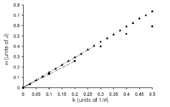
Figure 4: The collective-mode dispersion $\omega(\textbf{k})$ (triangles) calculated by the Bethe-Salpeter formalism for a 2D system with $\textbf{q}=q_{x}\textbf{e}_{x}$, $q_{x}=0.06\pi/a$, $\mu_{\uparrow}=3.5J$, $\mu_{\downarrow}=2.5J$, $\Delta=0.27J$, $U=3J$ and $T=0.07J$. The speed of sound to the direction of the x axis is $c=1.48Ja/\hbar$. The squire points are taken from Ref. [SF19, ], and the corresponding speed of sound is $c=1.29Ja/\hbar$.

IV Discussion

We have studied the Nambu-Goldstone excitation spectrum and the corresponding speed of sound of an interacting Fermi mixture of Lithium-6 and Potassium-40 atoms Fermi gases in deep optical lattices by using the Bethe-Salpeter equation in the GRPA. The generalized single-particle Green’s function, used in our numerical calculations, takes into account all possible thermodynamic averages. In view of the fact that most of the previous numerical calculations are based on the Nambu-Gor’kov single-particle Green’s function (6) which leads to the $4\times 4$ secular determinant, one may well ask whether the collective-mode dispersion, defined by the secular determinant $Z_{4}$, is significantly different in comparison to the dispersion obtained with the secular determinant $Z_{8}$.

To answer this question, we have calculated the collective-mode dispersion relation $\omega(Q_{x})$ using the $4\times 4$ determinant (12). The numerical results show that the determinant $Z_{4}$ and the determinant $Z_{8}$, both provide almost the same dispersions; the difference is about $2\%-7\%$ in the interval $-0.1\pi/a<Q_{x}<0.1\pi/a$, and less than $1\%$ out of this interval.

In conclusion, we briefly discuss the collective-mode dispersion of a population-imbalanced atomic Fermi gas obtained in Ref. [SF19, ] by applying the Kadanoff-Baym density response formalism. To the best of our knowledge this is the first paper in which the collective-mode dispersion and the corresponding speed of sound are calculated starting from the generalized single-particle Green’s function. However, it is not difficult to prove analytically that the location of the poles of the density response function is provided by the secular determinant $Z_{4}$. Since the Fock contributions to the electron self-energy are the same in the BS and the Kadanoff-Baym approaches, the only reason to have $Z_{4}$ instead of $Z_{8}$ is in the corresponding Hartree contributions. According to the Ref. [SF19, ], the Hartree contributions are $-UG_{22}(1;2)$, $-UG_{11}(1;2))$, $-UG_{44}(1;2)$, $-UG_{33}(1;2)$, while the Hartree terms $(U/2)(G_{44}(1;2)-G_{22}(1;2))$, $(U/2)(G_{33}(1;2)-G_{11}(1;2))$, $(U/2)(G_{22}(1;2)-G_{44}(1;2))$, and $(U/2)(G_{11}(1;2)-G_{33}(1;2))$ are obtained from the SD equations without any approximation. In other words, the Hartree contribution to the electron self-energy, as defined by Eq. (24), is an exact result. The dispersion obtained by means of the secular determinant $Z_{8}$ is presented in Fig. 4. In the range of small $k$, we find a difference of about $15\%$ between the speed of sound obtained by means of $Z_{8}$ secular determinant, and the speed of sound, calculated in Ref. [SF19, ]. The figure also indicates that the difference between the two dispersion curves tends to increase with $k$, reaching $25\%$ at $k=0.5/a$.

References

- (1) P. Fulde, and R. A. Ferrell, Phys. Rev. 135, A550 (1964).
- (2) A. I. Larkin, and Y. N. Ovchinnikov, Zh. Eksp. Teor. Fiz., 47, 1136 (1964) [Sov. Phys. JETP 20, 762 (1965)].
- (3) Y. Nambu, Phys. Rev. Lett., 4,380 (1960).
- (4) J. Goldstone, Nuovo Cimento, 19,154 (1961).
- (5) J. K. Chin, D. E. Miller, Y. Liu, C. Stan, W. Setiawan, C. Sanner, K. Xu, and W. Ketterle, Nature (London) 443, 961 (2006).
- (6) M.W. Zwierlein, A. Schirotzek, C. H. Schunck, and W. Ketterle, Science 311, 492 (2006).
- (7) G. B. Partridge, W. Li, R. I. Kamar, Y. Liao, and R. G. Hulet, Science 311, 503 (2006).
- (8) M.W. Zwierlein, C. H. Schunck, A. Schirotzek, and W. Ketterle, Nature (London) 442, 54 (2006).
- (9) Y. Shin, C. Schunck, A. Schirotzek, and W. Ketterle, Nature (London) 451, 689 (2008).
- (10) Y. Liao, A. S. C. Rittner, T. Paprotta, W. Li, G. B. Partridge, R. G. Hulet, S. K. Baur, and E. J. Mueller, Nature (London) 467, 567 (2010).
- (11) S. Nascimb‘ene, N. Navon, K. J. Jiang, L. Tarruell, M. Teichmann, J. McKeever, F. Chevy, and C. Salomon, Phys. Rev. Lett. 103, 170402 (2009).
- (12) S. Nascimb‘ene, N. Navon, K. Jiang, F. Chevy, and C. Salomon, Nature (London) 463, 1057 (2010).
- (13) G. M. Bruun and B.R. Mottelson, Phys. Rev. Lett. 87, 270403 (2001).
- (14) W. Hofstetter, J. I. Cirac, P. Zoller, E. Demler, and M. D. Lukin, Phys. Rev. Lett. 89, 220407 (2002).
- (15) Y. Ohashi, and A. Griffin, Phys. Rev. A 67, 063612 (2003).
- (16) G. Orso and G.V. Shlyapnikov, Phys. Rev. Lett. 95, 260402 (2005).
- (17) L. P. Pitaevskii, S. Stringari, and G. Orso, Phys. Rev. A 71, 053602 (2005).
- (18) W. Hofstetter Phil. Mag., 86, 1891 (2006).
- (19) W. Yi and L.-M. Duan, Phys. Rev. A 73, 063607 (2006).
- (20) T. Koponen, J.-P. Martikainen, J. Kinnunen, and P. Törmä1, Phys. Rev. A 73, 033620 (2006).
- (21) T. Koponen, J.-P. Martikainen, J. Kinnunen, L¿ M. Jensen, and P. Törmä1, New Journal of Physics 8, 179 (2006).
- (22) M. Iskin and C. A. R. Sá de Melo, Phys. Rev. Lett. 99, 080403 (2007).
- (23) T. K. Koponen, T. Paananen, J.-P. Martikainen, and P. Törmä, Phys. Rev. Lett. 99, 120403 (2007).
- (24) M. M. Parish, S. K. Baur, E. J. Mueller, and D. A. Huse, Phys. Rev. Lett. 99, 250403 (2007).
- (25) R. Haussmann, W. Rantner, S. Cerrito, and W. Zwerger, Phys. Rev. A 75, 023610 (2007).
- (26) T. Paananen, T. K. Koponen, P. Törmä, and J. P. Martikainen, Phys. Rev. A 77, 053602 (2008).
- (27) I. Bloch, J. Dalibard, and W. Zwerg, Rev. Mod. Phys. 80, 885 (2008).
- (28) T. Paananen, J. Phys. B: At. Mol. Opt. Phys. 42, 165304 (2009).
- (29) Ai-Xia Zhang and Ju-Kui Xue, Phys. Rev. A 80, 043617 (2009).
- (30) T. K. Koponen, T. Paananen, and P. Törmäl, Phys. Rev. Lett. 102, 165301 (2009).
- (31) J. M. Edge and N. R. Cooper, Phys. Rev. Lett. 103, 065301 (2009).
- (32) M. Iskin and C. A. R. Sá de Melo, Phys. Rev. Lett. 103, 165301 (2009).
- (33) Y. Yunomae, I. Danshita, D. Yamamoto, N Yokoshi, and S Tsuchiya, Journal of Physics: Conference Series 150, 032128 (2009).
- (34) Y. Yunomae, D. Yamamoto, I. Danshita, N Yokoshi, and S Tsuchiya, Phys. Rev. A 80, 063627 (2009).
- (35) R. Ganesh, A. Paramekanti and A. A. Burkov, Phys. Rev. A 80, 043612 (2009).
- (36) Cheng Zhao, Lei Jiang, Xunxu Liu, W. M. Liu, Xubo Zou, and Han Pu, Phys. Rev. A 81, 063642 (2010).
- (37) Z. Koinov, R. Mendoza and M. Fortes, Phys. Rev. Lett. 106 100402 (2011).
- (38) M. O. J. Heikkinen and P. Törmä, Phys. Rev. A 83, 053630 (2011).
- (39) L. M. Sieberer and M. A. Baranov, Phys. Rev. A 84, 063633 (2011).
- (40) J. Kajala, F. Massel, and P. Törmä, Phys. Rev. A 84, 041601(R)(2011).
- (41) Dong-Hee Kim, and P. Törmä, Phys. Rev. B 85, 180508(R)(2012).
- (42) M. O. J. Heikkinen, Dong-Hee Kim, and P. Törmä, Phys. Rev. B 87, 224513 (2013).
- (43) M. Iskin, Phys. Rev. A 88, 013631 (2013).
- (44) K. Seo, C. Zhang, and S. Tewari, Phys. Rev. A 88, 063601 (2013).
- (45) R. Mendoza, M. Fortes, M. A. Solís and Z. Koinov, Phys. Rev. A. 88 033606 (2013).
- (46) A. Korolyuk, J. J. Kinnunen, and P. Törmä, Phys. Rev. B 89, 013602 (2014).
- (47) Shaoyu Yin,1 J.-P. Martikainen, and P. Törmä, Phys. Rev. B 89, 014507 (2014).
- (48) J. Schwinger, Phys. Rev., 82, 914 (1951).
- (49) F. J. Dyson, Phys. Rev., 75, 1736 (1949).
- (50) H. A. Bethe and E. E. Salpeter, Phys. Rev., 82, 309 (1951); ibit. 84, 1232 (1951).
- (51) R. Cotê and A. Griffin, Phys. Rev. B 37, 4539 (1988).
- (52) R. Cotê and A. Griffin, Phys. Rev. B, 48, 10404 (1993).
- (53) H. Chu and Y. C. Chang, Phys. Rev. B 54, 5020 (1996).
- (54) Z. Koinov, Phys. Rev. B 72, 085203 (2005).
- (55) R. Combescot, M. Yu. Kagan, and S. Stringari, Phys. Rev. A 74, 042717 (2006).
- (56) Z. G. Koinov, Physica Status Solidi (B), 247 ,140 (2010); Physica C 407, 470 (2010).
- (57) Z. G. Koinov, Ann. Phys. (Berlin) 522, 693 (2010).
- (58) P. W. Anderson, Phys. Rev. 112, 1900 (1958).
- (59) G. Rickayzen, Phys. Rev. 115, 795 (1959).
- (60) L. Belkhir and M. Randeria, Phys. Rev. B 49, 6829 (1994).
- (61) G. Baym and L. P. Kadanoff, Phys. Rev., 124, 287 (1961).
- (62) G. Baym, Phys. Rev. 127, 1391 (1962).
- (63) C. Macêdo, and M. Coutinho-Filho, Phys. Rev. B, 43, 13515 (1991).
- (64) C. De Dominicis and P. Martin, J. Math. Phys., 5, 430 (1964).
- (65) C. Itzykson and J. Zuber, Quantum Field Theory, McGraw-Hill, NY 1980.
- (66) K. Maki, p. 1035, in ”Superconductivity”, edited by R.D. Parks, Marcel Dekker, Inc., New York, (1969).
- (67) P. Pieri, D. Neilson, and G. C. Strinati, Phys. Rev. B 75, 113301 (2007).
- (68) T. Hakioğlu and M. Şahin, Phys. Rev. Lett. 98, 166405 (2007).
- (69) T. Zhou and C. S. Ting, Phys. Rev. B 80, 224515 (2009).
- (70) Xian-Jun Zuo and Chang-De Gong, EPL, 86 47004 (2009).
- (71) H. Shimahara Phys. Rev. B 80, 214512 (2009).
- (72) A. Romano et al, Phys. Rev. B 81, 064513 (2010).
- (73) R. Ikeda, Phys. Rev. B 81, 060510(R) (2010).
- (74) M. M. Maśka et al, Phys. Rev. B 82, 054509 (2010).
- (75) Tung-Lam Dao, A. Georges, and M. Capone, Phys. Rev. B 76, 104517 (2007),
- (76) Q. Chen et al, Phys. Rev. B 75, 014521 (2007).
- (77) Xia-Ji Liu, H. Hu, and P. D. Drummond, Phys. Rev. A 76, 043605 (2007).
- (78) M. Rizzi, et al, Phys. Rev B 77, 245105 (2008).
- (79) Xia-Ji Liu, Hui Hu, and P. D. Drummond, Phys. Rev. A 78, 023601 (2008).
- (80) M. Reza Bakhtiari, M. J. Leskinen, and P. Törma, Phys. Rev. Lett. 101, 120404 (2008),
- (81) A. Lazarides and B. Van Schaeybroec Phys. Rev. A 77, 041602 (2008).
- (82) X. Cui and Y. Wang, Phys. Rev. B 79, 180509(R) (2009). A. Mishra and H. Mishra, Eur. Phys. J. D 53, 75 (2009);.
- (83) B. Wang, Han-Dong Chen, and S. Das Sarma, Phys. Rev. A 79, 051604(R) (2009).
- (84) Y. Yanase, Phys. Rev. B 80, 220510(R) (2009).
- (85) A. Ptok, M. Máska, and M. Mierzejewski, J. Phys.: Condens. Matter 21, 295601 (2009).
- (86) Yan Chen et al, Phys. Rev. B 79, 054512 (2009); Yen Lee Loh and N. Trivedi, Phys. Rev. Lett. 104, 165302 (2010).
- (87) A. Korolyuk, F. Massel, and P. Törma, Phys. Rev. Lett. 104, 236402 (2010).
- (88) F. Heidrich-Meisner et al, Phys. Rev. A 81, 023629 (2010).
- (89) S. K. Baur, J. Shumway, and E. J. Mueller, Phys. Rev. A 81, 033628 (2010).
- (90) A. Korolyuk, F. Massel, and P. Törmä, Phys. Rev. Lett. 104, 236402 (2010).
- (91) M. J. Wolak et al, Phys. Rev. A 82, 013614 (2010).
- (92) L. Radzihovsky and D. Sheehy, Rep. Prog. Phys. 73, 076501 (2010)
- (93) J. M. Edge and N. R. Cooper, Phys. Rev. Lett. 103, 065301 (2009); Phys. Rev. A 81, 063606 (2010).
- (94) A. Sedrakian and D. H. Rischke, Phys. Rev. D 80, 074022 (2009).
- (95) G. Sarma, J. Phys. Chem. 24, 1029 (1963).
- (96) P. F. Bedaque, H. Caldas, and G. Kupak, Phys. Rev. Lett. 91, 247002 (2003).
- (97) H. Caldas, Phys Rev. A 69, 063602 (2004).
- (98) H. Caldas, C. W. Morais and A. L. Mota, Phys. Rev. D 72, 045008 (2005).
- (99) S. Sachdev and K. Yang, Phys. Rev. B 73, 174504 (2006).
- (100) D.E. Sheehy, L. Radzihovsky, Phys. Rev. Lett. 96, 060401 (2006).
- (101) L. He, M. Jin, and P. Zhuang, Phys. Rev. B 74, 024516 (2006).
- (102) D.E. Sheehy and L. Radzihovsky, Ann. Phys. (N.Y.) 322, 1790 (2007).
- (103) M. Iskin and C.A.R. S de Melo, Phys. Rev. A 78, 013607 (2008).
- (104) S. Palh, and Z. Koinov, J Low. Temp. Phys., 176, 113 (2014)