Determining X-Ray Source Intensity and Confidence Bounds in Crowded Fields

Abstract

We present a rigorous description of the general problem of aperture photometry in high energy astrophysics photon-count images, in which the statistical noise model is Poisson, not Gaussian. We compute the full posterior probability density function for the expected source intensity for various cases of interest, including the important cases in which both source and background apertures contain contributions from the source, and when multiple source apertures partially overlap. A Bayesian approach offers the advantages that it allows one to (a) include explicit prior information on source intensities, (b) propagate posterior distributions as priors for future observations, and (c) use Poisson likelihoods, making the treatment valid in the low counts regime. Elements of this approach have been implemented in the Chandra Source Catalog.

1 Introduction

A common problem in astronomy is the estimate of the intensity of a celestial source, using digital image data that also include contaminating contributions from sky background and nearby sources. In optical, infrared, and ultraviolet images, there are typically sufficient photon events per pixel that a Gaussian statistical noise model can be assumed, and one may fit a model spatial profile, including telescope response and any intrinsic source extent, to the observed event distribution (see e.g. Stetson, 1987). In X-ray and $\gamma$-ray images however, there are typically few events per pixel, even for long exposures. Moreover, the telescope response or point spread function (PSF) may vary significantly with photon energy and with location in the field-of-view. Its size may range from approximately one image pixel near the optical axis to several tens of pixels at large off-axis distances. In such cases, model-fitting to the sparse photon data can become difficult, or at least computationally expensive, and researchers often resort to simpler aperture photometry techniques. These involve counting photon events in a region, or aperture, centered on the nominal source location, with background determined from event counts in near-by source-free regions. Net counts are then multiplied by correction factors to convert counts to flux for an assumed spectral model and to correct for losses due to detector/telescope efficiency or apertures whose sizes do not enclose the full PSF at the source location. The resulting intensities or fluxes are typically simple algebraic functions of the raw aperture counts, and their errors are often estimated by using simple propagation of error techniques which assume a Gaussian statistical noise model.

A number of authors have attacked the problem using Bayesian statistical techniques, which can naturally incorporate a Poisson noise model. Loredo (1992) first pointed out the advantages of such techniques to determine x-ray intensities for isolated sources, and Kraft, Burrows & Nousek (1991) used a Bayesian formalism to determine confidence bounds on x-ray intensities. Recently, Laird et al. (2009) considered the astronomically interesting case in which the prior distribution for source intensity is given by a $logN-logS$ distribution, and showed that this can naturally account for the sampling bias in intensity near detection threshold. However, these treatments all assume that background is either negligible or known and that background apertures are uncontaminated by source counts. Weisskopf et al. (2007) carried out a likelihood-based analysis that treats the case where both source and background apertures contain source contributions, and allows for uncertainties in background measurements. However, their analysis only treats the case of isolated sources and does not consider any prior information on source or background intensity.

In this paper we present a full Bayesian treatment for the problem and explicitly account for contributions from multiple sources in both source and background apertures. We emphasize that we are addressing the problem of estimating the range in which a source intensity is likely to be found, at some given probability level, not the probability that the source is real. The latter is an equally important but separate problem (Kashyap et al., 2010). We begin in Section 2 with a discussion of the Maximum Likelihood solution to ground the user in our terminology. In Section 3.1 we present our Bayesian formalism for the case of an isolated source and extend the treatment to multiple sources in Section 3.2. In Section 4, we consider some examples and explore the range of situations where our treatment is useful, using simulations. We present the detailed mathematics of our derivations in appendices.

2 Maximum Likelihood Estimate for Net Counts

We derive here the relevant formulae for computing maximum likelihood estimates for net counts for an unresolved source or sources from quantities obtained in aperture photometry measurements. We limit our discussion to net counts but note that other quantities such as source rate or flux can also be accommodated by introducing the appropriate conversion factors (e.g. exposure or effective area). This section essentially paraphrases the results derived in Appendix A of Weisskopf et al. (2007), modified only to accomodate the different variables and terms that we use throughout the paper. These are defined in Table 1.

2.1 An Isolated Source

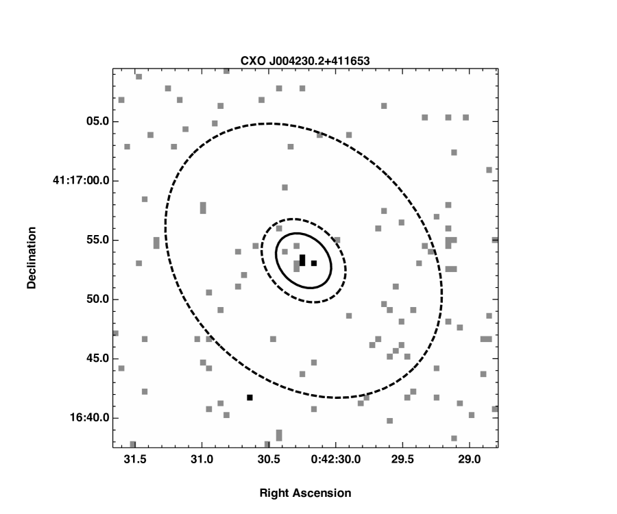
Figure 1: Source (solid ellipse) and background apertures (dashed ellipses) for an isolated X-ray source, from data obtained from Release 1.1 of the Chandra Source Catalog (Evans et al., 2010). The background aperture has been modified slightly to illustrate the use of a detached aperture. For this source, C=12, $\Omega_{s}$=67.74 $\,pix^{2}$, f=0.93, B=33, $\Omega_{b}$=1537.41 $\,pix^{2}$, and g=0.03.

We consider first the simple case of a single, isolated source, for which suitable source and background apertures can be constructed without encountering other contaminating sources. The situation is shown in Figure 1. For clarity, we omit the source subscript $i$. Although apertures may be of arbitrary shape, subject to the limitation that $\int_{R}psf(X,Y,x,y)dxdy$ exist, we use apertures bounded by ellipses since they roughly approximate the general shape of psfs for typical x-ray telescopes.

The ability to construct a suitable background aperture depends on a balance of competing factors. In x-ray images with very low background densities, it may be necessary to require $\Omega_{b}\gg\Omega_{s}$ in order to obtain an accurate measure of the background. One may also wish to separate or detach the source and background apertures, as we show in Figure 1, to minimize the source contribution to the background aperture. However, spatial variations in the background and a high source density may force a smaller background aperture situated close to the source, in order to approximate the background with a constant value and to treat the source as isolated.

Assuming that appropriate apertures can be defined, the observed counts $C$ in the source aperture and $B$ in the background aperture may be treated as samples from Poisson distributions with means $\mu_{s}=fs+\Omega_{s}b$ and $\mu_{b}=gs+\Omega_{b}b$, where $f$ and $g$ are PSF fractions in source and background apertures with areas $\Omega_{s}$ and $\Omega_{b}$, and $s$ and $b$ are true source counts and background density, respectively. Since $C$ and $B$ are statistically independent, the total probability of obtaining $C$ counts in source aperture $R_{s}$ and $B$ counts in background aperture $R_{b}$ is given by

$$P(C,B|\mu_{s},\mu_{b})=Pois(\,C\,|\,\mu_{s})\,Pois(\,B\,|\,\mu_{b})=\frac{\mu_{s}^{C}}{\Gamma(C+1)}e^{-\mu_{s}}\frac{\mu_{b}^{B}}{\Gamma(B+1)}e^{-\mu_{b}}.$$ (1)

Defining the log-likelihood function $L$ as

$$L=ln[P(C,B|\mu_{s},\mu_{b})]=C\,ln(\mu_{s})-\mu_{s}+B\,ln(\mu_{b})-\mu_{b}-ln[\Gamma(C+1)]-ln[\Gamma(B+1)],$$ (2)

we obtain maximum-likelihood estimators for $s$ and $b$ by requiring $\frac{\partial L}{\partial s}=0$ and $\frac{\partial L}{\partial b}=0$ . Both conditions are are satisfied by the solution to the two simultaneous linear equations

$$C = \mu_{s}=fs+\Omega_{s}b$$

$$B = \mu_{b}=gs+\Omega_{b}b.$$

The maximum-likelihood estimators for $s$ and $b$ (cf. Weisskopf et al. (2007), eq. A12 & A13) are thus

$$\hat{s} = \frac{C\Omega_{b}-B\Omega_{s}}{f\Omega_{b}-g\Omega_{s}}$$

$$\hat{b} = \frac{Bf-Cg}{f\Omega_{b}-g\Omega_{s}}.$$

When $C$ and $B$ are large, so that we can assume a Gaussian statistical model, we can estimate the error in $\hat{s}$ and $\hat{b}$ using simple propagation of errors:

$$\sigma_{\hat{s}}^{2} = \frac{C\Omega_{b}^{2}+B\Omega_{s}^{2}}{(f\Omega_{b}-g\Omega_{s})^{2}}$$

$$\sigma_{\hat{b}}^{2} = \frac{Bf^{2}+Cg^{2}}{(f\Omega_{b}-g\Omega_{s})^{2}}.$$

2.2 Multiple Sources

Next, we consider the case in which there are two or more sources which contribute to the counts in the source and background apertures. The situation is illustrated in Figure 2. If the source apertures overlap, as is the case for two of the sources here, events in the overlap region should be attributed to only one of the overlapping source apertures, to preserve the statistical independence of the aperture counts. Then, for $n$ sources, the log-likelihood function $L$ is a simple extension to Equation 2:

$$L=\sum_{i=1}^{n}\left\{C_{i}\,ln(\mu_{s_{i}})-\mu_{s_{i}}-ln[\Gamma(C_{i}+1)]\right\}+B\,ln(\mu_{b})-\mu_{b}-ln[\Gamma(B+1)],$$ (6)

and the maximum-likelihood estimators for $s_{i}$ and $b$ are obtained by requiring that $\frac{\partial L}{\partial s_{i}}=0$ and $\frac{\partial L}{\partial b}=0$ . These conditions are satisfied by the solution to the set of $n+1$ simultaneous linear equations (cf. Kashyap et al., 1994)

$$C_{i} = \mu_{s_{i}}=\sum_{j=1}^{n}f_{ij}s_{j}+\Omega_{s_{i}}b$$

$$B = \mu_{b}=\sum_{i=1}^{n}g_{i}s_{i}+\Omega_{b}b.$$

Equation LABEL:eq:ML-mult can be written in matrix form as $\overline{C}=\overline{\overline{F}}\times\overline{S,}$ where vectors $\overline{C}$ and $\overline{S}$ are given by

$$\overline{C} = (C_{1},\ldots C_{n},\,B)$$

$$\overline{S} = (s_{1},\ldots s_{n},\,b),$$

and the matrix $\overline{\overline{F}}$ is given by

$$\overline{\overline{F}} = \begin{bmatrix}f_{11}&\cdots&f_{1n}&\Omega_{s_{1}}\\ \vdots&\ddots&\vdots&\vdots\\ f_{n1}&\cdots&f_{nn}&\Omega_{s_{n}}\\ g_{1}&\cdots&g_{n}&\Omega_{b}\end{bmatrix}.$$

The solution is then $\overline{S}=\overline{\overline{F^{-1}}}\times\overline{C}$ , where $\overline{\overline{F^{-1}}}$ is the inverse of $\overline{\overline{F}}$, or

$$\hat{s}_{k} = \sum_{j=1}^{n}F_{kj}^{-1}C_{j}+F_{k,n+1}^{-1}B$$

$$\hat{b} = \sum_{j=1}^{n}F_{n+1,j}^{-1}C_{j}+F_{n+1,n+1}^{-1}B,$$ (8)

and the uncertainties are given by

$$\sigma_{\hat{s}_{k}}^{2} = \sum_{j=1}^{n}(F_{kj}^{-1})^{2}C_{j}+(F_{k,n+1}^{-1})^{2}B$$

$$\sigma_{\hat{b}}^{2} = \sum_{j=1}^{n}(F_{n+1,j}^{-1})^{2}C_{j}+(F_{n+1,n+1}^{-1})^{2}B.$$ (9)

3 Bayesian Formalism

We now consider the problem from a Bayesian perspective. Our goal is to derive relations for the posterior probability distributions for background and source intensities which can be used to determine intensities and credible regions analagous to the quantities described in Equations LABEL:eq:ML-single,LABEL:eq:ML-single-sigma,8, and 9.

3.1 An Isolated Source

We consider again the situation shown in Figure 1. We still assume that the counts in the source and background apertures are drawn from independent Poisson processes, but now use Bayes’ Theorem to express the posterior probability distributions for $\mu_{s}$and $\mu_{b}$, the total intensities due to both source and background in the respective apertures:

$$P(\mu_{s},\,\mu_{b}|\,C,\,B) = \frac{P(\mu_{s},\,\mu_{b})\,P(C,\,B\,|\,\mu_{s},\,\mu_{b})}{P(C,\,B)}$$

$$= \frac{P(\mu_{s})P(\mu_{b})}{P(C,\,B)}\,\frac{\mu_{s}^{C}}{\Gamma(C+1)}e^{-\mu_{s}}\frac{\mu_{b}^{B}}{\Gamma(B+1)}e^{-\mu_{b}},$$

where we have used the Poisson Likelihoods from Equation 1 and have taken advantage of the statistical independence of $C\,,B$ and $\mu_{s}\,,\mu_{b}$. For the prior probabilities for $\mu_{s}$ and $\mu_{b}$ we use $\gamma$-distributions of the form

$$P(\mu_{s}) = \frac{\beta_{s}^{\alpha_{s}}\mu_{s}^{\alpha_{s}-1}e^{-\beta_{s}\mu_{s}}}{\Gamma(\alpha_{s})},$$

$$P(\mu_{b}) = \frac{\beta_{b}^{\alpha_{b}}\mu_{b}^{\alpha_{b}-1}e^{-\beta_{b}\mu_{b}}}{\Gamma(\alpha_{b})}.$$

These distributions are referred to as conjugate priors for Poisson Likelihood functions, since they result in posterior distributions of the same functional form (Raiffa & Schlaifer, 1961). They are highly flexible functions that can be used to specify the Poisson intensity a priori. The number of counts is specified as $\alpha-1$, and the relative areas and exposure times are specified via $\beta$. In the limit in which $\alpha_{s}\,,\alpha_{b}\rightarrow 1$ and $\beta_{s}\,,\beta_{b}\rightarrow 0$, these approach non-informative, flat priors.

The joint posterior probability distribution is then

$$P(\mu_{s},\,\mu_{b}|\,C,\,B\,) = \mu_{s}^{C+\alpha_{s}-1}e^{-\mu_{s}(1+\beta_{s})}\mu_{b}^{B+\alpha_{b}-1}e^{-\mu_{b}(1+\beta_{b})}\times$$

$$\frac{1}{P(C,\,B)}\frac{\beta_{s}^{\alpha_{s}}\beta_{b}^{\alpha_{b}}}{\Gamma(\alpha_{s})\Gamma(C+1)\Gamma(\alpha_{b})\Gamma(B+1)}.$$

The evidence term $P(C,B)$ is determined by the standard normalization requirement

$$\intop_{0}^{\infty}d\mu_{s}\intop_{0}^{\infty}d\mu_{b}P(\mu_{s},\,\mu_{b}|\,C,\,B\,)=1,$$ (13)

and the posterior distribution $P(s)$ is determined by changing variables from $\mu_{s}\,,\mu_{b}$ to $s\,,b$ and then marginalizing over all values of b:

$$P(s\,|C,B)=\intop_{0}^{\infty}db\,P(s,b\,|C,B).$$ (14)

The mathematical details are provided in Appendix A. The final result is

$$P(s\,|C,\,B) = (\Omega_{b}f-\Omega_{s}g)\times(1+\beta_{s})^{(C+\alpha_{s})}\,e^{-fs(1+\beta_{s})}\times(1+\beta_{b})^{(B+\alpha_{b})}\,e^{-gs(1+\beta_{b})}\times$$

$$\sum_{k=0}^{(C+\alpha_{s}-1)}\,\sum_{j=0}^{(B+\alpha_{b}-1)}\frac{(fs)^{k}\,\Omega_{s}^{(C+\alpha_{s}-1-k)}}{\Gamma(k+1)\Gamma(C+\alpha_{s}-k)}\times\frac{(gs)^{j}\,\Omega_{b}^{(B+\alpha_{b}-1-j)}}{\Gamma(j+1)\Gamma(B+\alpha_{b}-j)}\times$$

$$\frac{\Gamma(C+\alpha_{s}-k+B+\alpha_{b}-j-1)}{[\Omega_{s}(1+\beta_{s})+\Omega_{b}(1+\beta_{b})]^{(C+\alpha_{s}-k+B+\alpha_{b}-j-1)}}\,.$$

For the case of non-informative prior distributions, with $\alpha_{s}=\alpha_{b}=1$ and $\beta_{s}=\beta_{b}=0$,

$$P(s\,|C,\,B) = (\Omega_{b}f-\Omega_{s}g)\times\,e^{-fs}\times e^{-gs}\times$$

$$\sum_{k=0}^{C}\,\sum_{j=0}^{B}\frac{(fs)^{k}\,\Omega_{s}^{(C-k)}}{\Gamma(k+1)\Gamma(C-k+1)}\times\frac{(gs)^{j}\,\Omega_{b}^{(B-j)}}{\Gamma(j+1)\Gamma(B-j+1)}\times$$

$$\frac{\Gamma(C-k+B-j+1)}{(\Omega_{s}+\Omega_{b})^{(C-k+B-j+1)}}\,.$$

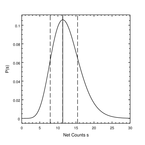
Figure 3: Posterior probability distribution for the source shown in Figure 1, evaluated using Equation 3.1. The distribution mode and 68% confidence bounds are indicated with vertical dashed lines. The Maximum Likelihood estimate is indicated by a solid vertical line.

We use Equation 3.1 to evaluate the posterior distribution for the source shown in Figure 1. The result is shown in Figure 3. We note that the mode of the posterior distribution is indistinguishable from the maximum likelihood estimate for net source counts, as should be expected, since we assumed non-informative or flat priors in deriving Equation 3.1. In such cases, as can be seen from Equation LABEL:bayestheorem, the posterior probability distribution reduces to the product of the likelihoods. We shall examine this topic in more detail in Section 4.

3.2 Multiple Sources

We now consider multiple sources from a Bayesian perspective. As before, Bayes’ Theorem is used to express the joint posterior probability distribution in terms of likelihoods and prior probabilities. The details are provided in Appendix B. The marginalized posterior probability distribution for source $s_{i}$ is given in Equation B4 as

$$P(s_{i}\,|\,C_{1}\ldots C_{n}\,,\,B)ds_{i}=K^{\prime}\dotsintop_{b\,,\,s_{j}\neq s_{i}}db\,P(\mu_{b})\,Pois(B\,|\,\mu_{b})\prod_{i=1}^{n}ds_{i}P(\mu_{s_{i}})\,Pois(C_{i}\,|\,\mu_{s_{i}}).$$ (17)

A similar result holds for $P(b\,|\,C_{1}\ldots C_{n}\,,\,B)db$, where integration is now over all sources, but not background.

We again assume $\gamma$-distributions for priors, so that, e.g.,

$$P(\mu_{s_{i}})=\frac{\beta_{i}^{\alpha_{i}}\mu_{s_{i}}^{\alpha_{i}-1}e^{-\beta_{i}\mu_{s_{i}}}}{\Gamma(\alpha_{i})}.$$ (18)

Since binomial expansions of powers containing $\alpha_{i}$ are no longer used in evaluating marginalizing integrals (as in Appendix A, Equation LABEL:eq:binomial), the restriction that $\alpha_{i}$ and $\alpha_{b}$ be integers is lifted.

The multiplicative constants in the prior distributions can be absorbed into the single normalization constant $K^{\prime},$ yielding

$$P(s_{i}\,|\,C_{1}\ldots C_{n}\,,\,B)ds_{i}=K^{\prime}\dotsintop_{b\,,\,s_{j}\neq s_{i}}db\,\mu_{b}^{\alpha_{b}-1}e^{-\beta_{b}\mu_{b}}\,Pois(B\,|\,\mu_{b})\prod_{i=1}^{n}ds_{i}\mu_{s_{i}}^{\alpha_{i}-1}e^{-\beta_{i}\mu_{s_{i}}}\,Pois(C_{i}\,|\,\mu_{s_{i}}).$$ (19)

As seen in Figure 3, the posterior distributions are expected to be localized near the distribution mode, and to vary smoothly. In such cases, it may be possible to evaluate the integrand in Equation 19 on a suitable (n+1)-dimensional grid and evaluate the n-dimensional marginalization integral by repeated one-dimensional numerical integrations. In our web page, we present a sample Python program for doing just that, using the maximum-likelihood estimates of source counts and errors to define the parameters of the mesh. In the next section we use our code to explore a number of test cases.

4 Verification and Simulations

4.1 Exemplar Test Cases

In this section, we apply the procedure discussed at the end of the last section to two test cases, using data from real Chandra observations.

4.1.1 An Isolated Point Source

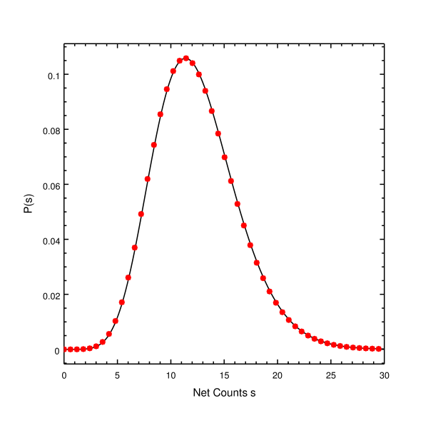
Figure 4: Comparison of posterior distributions computed from Equations 3.1 (solid black line) and 19 (red circles) for the example shown in Figure 1.

We begin with the simple case shown in Figure 1. As described at the end of Section 3.1, we computed $P(s\,|\,C,\,B)$ analytically for the aperture data given in the caption to Figure 1, using Equation 3.1, as implemented in the CIAO tool aprates. We now use our new sample code to compute $P(s\,|\,C,\,B)$ numerically from Equation 19. In both cases, we assumed non-informative $\gamma-$distribution priors with $\alpha=1$ and $\beta=0$. We compare the posterior distributions in Figure 4. The distributions are in excellent agreement, demonstrating that our numerical integration procedure and sample code produce results consistent with the analytical result in the simple case where both are applicable.

4.1.2 Sources in a Crowded Region

We next consider the four Chandra Source Catalog sources shown in Figure 2. All sources are treated at once, although only two have overlapping apertures. However, one of the remaining sources, r0115, is sufficiently bright that it may influence the background data even if its source aperture is excluded from the background. Source and background data for this case are listed in Table Determining X-Ray Source Intensity and Confidence Bounds in Crowded Fields. For the sources with overlapping source apertures, we have attributed counts and area in the overlap region to the fainter of the two sources, r0150.

Non-Informative Priors

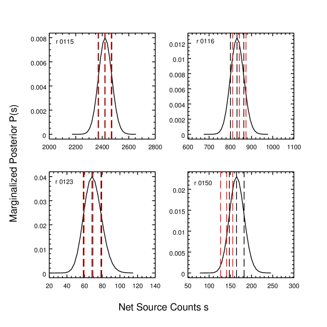
Figure 5: Posterior distributions for the four sources in Figure 2. Modes and 68% confidence bounds are indicated by black vertical dashed lines. Results from Release 1.1 of the Chandra Source Catalog are shown in red.

We first assume non-informative  $\gamma$-distribution priors for all sources and background, with $\alpha_{i}=1$ and $\beta_{i}=0$, so that we can compare our results with those of Release 1.1 of the Chandra Source Catalog (Evans et al., 2010). Our procedure yields the posterior distributions shown in Figure 5. To estimate confidence bounds, we approximate the mode of each distribution as the vertex of a quadratic function fit to the three highest points in the distribution. We then numerically integrate the sample posterior distribution above and below the mode until the $68\%$ confidence bounds are obtained. For the two isolated sources, r0115 and r0123, the modes and confidence bounds, (black dashed vertical lines), are in good agreement with those from Release 1.1 of the Chandra Source Catalog (red dashed vertical lines), in which all sources were treated independently. Results for the overlapping sources r0116 and r0150 differ, as expected, since data in the overlap area were excluded from the analysis in Release 1.1. At present, we only note that different results are obtained. In Section 4.2, we present results of simulations that demonstrate that the new procedure produces more accurate results than that used in Release 1.1.

Informative Priors

We examine the effect of using informative priors by dividing the time interval of the original data set into two halves, and using the posterior distributions from one half (computed assuming non-informative priors) to estimate the prior distributions for the second. To do this, we note that, from the definition of $\gamma$-distribution priors in Equation LABEL:eq:gamma-dist

$$\alpha = \frac{[E(\mu)]^{2}}{Var(\mu)}$$

$$\beta = \frac{E(\mu)}{Var(\mu)}$$

where

$$E(\mu) = \int_{0}^{\infty}d\mu\,\mu\,P(\mu)$$

$$Var(\mu) = E(\mu^{2})-[E(\mu)]^{2}.$$

Since the aperture quantities $\mu_{s_{i}},\,\mu_{b}$ are linear combinations of source and background intensities, as given in Equation LABEL:eq:ML-mult and Table 1, we may write

$$E(\mu_{s_{i}}) = \sum_{j=1}^{n}f_{ij}E(s_{j})+\Omega_{s_{i}}E(b)$$

$$Var(\mu_{s_{i}}) = \sum_{j=1}^{n}f_{ij}^{2}Var(s_{j})+\Omega_{s_{i}}^{2}Var(b)\,,$$

and similarly for $E(\mu_{b})$ and $Var(\mu_{b})$.

We thus compute $E(s_{i}),\,Var(s_{i}),\,E(b),\,$ and $Var(b)$ from Equation LABEL:eq:def_E_Var, using the marginalized posterior distributions $P(s_{i}\,|\,C_{1}\ldots C_{n}\,,\,B)$ and $P(b\,|\,\leavevmode\nobreak\ C_{1}\ldots\leavevmode\nobreak\ C_{n}\,,\,B)$ from the first half of the data set as the probability distributions, and use these to compute $E(\mu_{s_{i}}),\,Var(\mu_{s_{i}}),\,E(\mu_{b}),\,$ and $Var(\mu_{b})$ from Equation LABEL:eq:def_E. These quantities are then used to compute $\alpha_{s_{i}},\,\beta_{s_{i}},\,\alpha_{b},\,$ and $\beta_{b}$ from Equation LABEL:eq:def_alpha to define the prior distributions for analysis of the second half of the data set.

Our results are shown in Figure 6. We note that for all four sources the posterior distributions for the second half of the data set based on informative priors are narrower than the equivalent distributions based on non-informative priors, with modes consistent with the distributions derived from the full dataset, based on non-informative priors. Note that by adopting informative priors based on an analysis of the first half for the second half of the observation, we make an implicit assumption that the sources do not exhibit intrinsic variability; this assumption appears to be invalid for at least one of the sources, r0116.

Although it is tempting to err on the side of caution and include all sources which may contribute to data in the background aperture, there is a practical limit to the number of sources one can treat at once in the simple numerical integration scheme that we use. The mesh size grows geometrically with the number of sources, and must include an adequate number of points in any one dimension to allow accurate determination of the mode and confidence bounds. With a mesh size of $\sim 20-30$ per source, current experience indicates that fewer than 5 sources can be analyzed simultaneously without exceeding typical memory resources. For example, analysis of 5 sources (a 6-dimensional mesh including background) with a mesh size of 30 per source would require $\sim 5$ Gbytes to hold the joint posterior distribution in memory. In such cases, more sophisticated algorithms, such as Markov Chain Monte Carlo techniques, may be required to evaluate Equation 19. Alternatively, one may be able to ignore sources in the joint computation based on their relative contributions. For example, a source $j$ for which $g_{j}\lesssim 0.05$ and $f_{ij}\lesssim 0.05$ for all other sources $i$ can likely be ignored since that is typically the limit to which the point spread function is known.

4.2 Limits of Applicability

Finally we investigate in more detail the performance of our procedure using simulations. Our aim is to provide some comparison with other techniques, and to explore the ranges in relative source intensity and source separation for overlapping sources, for which our procedure yields reliable results.

4.2.1 Simulation Set-Up

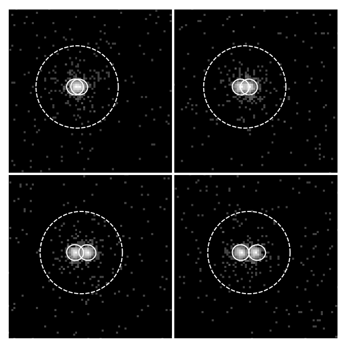
Figure 7: Simulated Chandra images of two point sources separated by $\Delta=0.5,1.0,1.5,2.0\times r_{90}$ at an off-axis angle of $\sim 0.5^{\prime}$. Each source has a true intensity of 1000 counts, and the mean background in the source aperture is $\sim 1$ count. Source apertures are constructed to enclose approximately 90% of the point spread function, and the background aperture (dashed circle with source apertures excluded) has an area 25 times greater than that of a single source aperture and is centered at a position halfway between the sources.

We build a systematic grid for simulations based on source separation, relative source intensity, and background level (D. Jones 2013, private communication). We used the CIAO tool ChaRT (Carter et al., 2003), Chandra raytracing software SAOTrace (Jerius et al., 2004), and CIAO tools psf_project_ray and dmcopy (Fruscione et al., 2006) to generate an ACIS image of the point spread function for a source at an off-axis angle of $\sim 0.5^{\prime}$ and pixel resolution of $\sim 0.25^{\prime\prime}$, using the metadata of Chandra observation 1575. We then used the two-dimensional modeling capabilities of $Sherpa$ (Freeman, Doe & Siemiginowska, 2001) to simulate pairs of sources separated by $\Delta=0.5,1.0,1.5,2.0\times r_{90}$, where $r_{90}$ is the average radius of an ellipse enclosing 90% of the encircled energy of the point spread function images, determined using the CIAO tool dmellipse. At the image locations chosen, $r_{90}\sim 1^{\prime\prime}$. At each separation, we considered a range of source intensities, with a bright source (source 1) with model counts $M_{1}=1000$ and a fainter source (source 2) with model counts $M_{2}=1000/r$. The relative intensity $r$ was chosen such that $log_{10}(r)=0,0.5,1,1.5,2,$ corresponding to $M_{2}$ values of $1000,\,316,\,100,\,31.6,$ and $10,$ respectively. Finally, we considered three different background levels, with model background in the 90% encircled energy source aperture for source 2 set to $b\times 900/r$, with $b=0.001,\,0.010,\,0.100$. For each combination of $\Delta,\,r,$ and $b$ , we used $Sherpa$ to simulate 1000 images with appropriate statistics applied for background and both source intensities. Examples for $r=1$ and $b=0.001$ are shown in Figure 7.

4.2.2 Results for New Procedure

We analyzed each image with our sample code, assuming non-informative priors for each source. We used the 90% encircled energy ellipses determined from $dmellipse$ to define the source apertures, and a circular region centered between the two sources with twenty-five times the area of a single source aperture to define the background aperture. Such background aperture sizes were typical of isolated point sources in Release 1.1 of the CSC. For each combination of $\Delta,\,r,$ and $b$ , and for each simulation $k$, we tabulated the modes, $S_{i}^{k}$, and 68% confidence bounds, $S_{i}^{k,-},S_{i}^{k,+}$, from the posterior probability distributions for each source $i$ in the image, and computed the average fractional error and fractional width, given by

$$fractional\,error_{i} = \frac{1}{1000}\times\sum_{k=1}^{1000}(\,S_{i}^{k}-M_{i}\,)/M_{i}$$

$$fractional\,width_{i} = \frac{1}{1000}\times\sum_{k=1}^{1000}(S_{i}^{k,+}-S_{i}^{k,-})/M_{i}$$

where $M_{i}$ refers to $M_{1}$ and $M_{2}$ for source 1 and 2, respectively.

For $\Delta\lesssim 1.5\,r_{90}\,$, there is substantial overlap in the source apertures, and we consider separately cases where overlap area $\Omega_{o}$ is assigned to the aperture of source 1 (Case 1) and source 2 (Case 2). To be specific, in Case 1 (for example), the aperture for source 1 is the full 90% encircled energy aperture with area $\Omega_{s_{1}}$, which includes area $\Omega_{o}$. All counts that fall within $\Omega_{s_{1}}$ are assigned to the aperture for source 1. Moreover, the aperture for source 2 is reduced in area to be $\Omega_{s_{2}}-\Omega_{o}$, and only counts that fall within this reduced area are assigned to the aperture for source 2. Case 2 is defined similarly. Fractional errors for both cases are shown in Figure Determining X-Ray Source Intensity and Confidence Bounds in Crowded Fields. We display the results as sets of density plots and contour of fractional error as a function of $\Delta$ and $log_{10}r$ for fixed values of $b,$ using radial basis linear interpolation on a $4\times 5$  $\Delta-log_{10}r$ mesh to provide smooth images and contours. Since the fractional errors, as defined in Equation LABEL:eq:fracerr, could be negative, we add a positive offset of 0.1 to all interpolated values to allow for a logarithmic scaling in the density plots. Contour values are corrected for the offset. Color bars and contours are the same for all plots. To provide a basis for comparison, we note that the intensity of an isolated point source with negligible background has a statistical uncertainty of $\sim 3\%$ for a $1000$ count source and $\sim 10\%$ for a $100$ count source.

As expected, fractional errors for source 1 are small over most of the range of $\Delta$ and $log_{10}r$, exceeding $+5\%$ only for $\Delta\lesssim 0.75\,r_{90}$ and $log_{10}r\lesssim 1$ (source 2 counts $\gtrsim 100$). Fractional errors for the fainter source 2 are larger, and exceed $\sim+50\%$ for sources fainter than $\sim 100$ counts or closer than $\sim r_{90}$ to source 1. It is interesting to note that Case 1 yields better results for source 2 than Case 2 does. For example, in Case 2 the fractional errors are in general larger in the region $\Delta\lesssim 1.0\,r_{90}$ and $log_{10}r\gtrsim 1.5$ than in Case 1, and the area in the density plots with fractional errors greater than $\sim+5\%$ is larger in Case 2 than in Case 1. We attribute this somewhat counter-intuitive efffect to the fact that the source 1 intensity, and hence its contribution to other aperture is more accurately determined when overlap area (and hence all counts) is assigned to its aperture.

Finally, in Figure Determining X-Ray Source Intensity and Confidence Bounds in Crowded Fields, we show results for fractional widths of the posterior probability distributions, displayed in a fashion similar to that used for fractional errors, except that since the widths are positive-definite quantities, no offset is added in displaying the density plots. For comparison, the $\pm 1\sigma$ width for a $1000$ count isolated point source with negligible background is $\sim 6\%$. We note again that better results for the fainter source 2 are achieved for Case 1. For example, the fractional widths are in general smaller in the region $\Delta\lesssim 1.0\,r_{90}$ and $log_{10}r\gtrsim 1.5$ than in Case 2, and the area in the density plots with fractional widths greater than $\sim+50\%$ is larger in Case 2 than in Case 1.

We emphasize that in our approach to resolving overlapping apertures, we do not assign counts to particular sources, but rather to particular apertures which have been modified to eliminate the overlap. Estimated counts in all apertures, as indicated in Equation LABEL:eq:ML-mult and Table 1, are modelled as a linear combination of background and all source intensities, with proportionality constants determined by psf contributions for sources and aperture area for background. Although it is possible to treat the overlap area as an additional aperture, this significantly complicates the mathematical treatment of the problem, and we don’t consider it here. We note that the major differences between Case 1 and Case 2, as indicated in Figure Determining X-Ray Source Intensity and Confidence Bounds in Crowded Fields, occur for $\Delta<\sim 1$. As a point of reference, in Release 1 of the Chandra Source Catalog (Evans et al., 2010), these close pairs amounted to fewer than $\sim 1\%$ of the total number of sources on average, although the fraction could be significantly larger in dense stellar clusters and nuclei of galaxies.

The approach of Broos et al. (2010) is similar to our Case 1, in that the aperture of the brighter source remains unchanged, while that of the fainter source is reduced. However, differences in the details of the reduced apertures may lead to somewhat different results.

4.2.3 Comparison with Maximum Likelihood Results

We also computed the Maximum Likelihood values for source intensity and uncertainty for both sources in each simulated image, using Equations 8 and 9. We then computed average fractional errors and widths as in Equation LABEL:eq:fracerr, substituting $\hat{s}_{k}$ for $S^{k}$ and $2\times\sigma_{\hat{s}_{k}}$ for $(S^{k,+}-S^{k,-})$. Cases 1 and 2 were defined as before. Our results are shown in Figures Determining X-Ray Source Intensity and Confidence Bounds in Crowded Fields and Determining X-Ray Source Intensity and Confidence Bounds in Crowded Fields, which may be compared to Figures Determining X-Ray Source Intensity and Confidence Bounds in Crowded Fields and Determining X-Ray Source Intensity and Confidence Bounds in Crowded Fields, respectively. The fractional errors for Source 1 and the fractional widths for both sources are, in fact, comparable to those determined using our procedure, for both Case 1 and Case 2. This might be expected, since we used non-informative priors in our current analysis, and, as noted at the end of Section 3.1, in such cases the Bayesian formalism reduces to the Maximum Likelihood one. However, for the fainter Source 2, the Maximum Likelihood average fractional errors are, in fact, much lower than those computed using our procedure in the region $\Delta\lesssim 1.5\,r_{90}$ and $log_{10}r\gtrsim 1.0$ (Source 2 counts $<100$). We attribute this to the fact that, although we use “non-informative” $\gamma-$distribution priors with $\alpha=1$ and $\beta=0$, we do take advantage of some prior information in our procedure, namely, the implicit assumption that all source intensities are non-negative. For bright sources, this prior information is of little significance, but for faint sources with few counts near brighter sources, it could be. In contrast, Maximum Likelihood estimators for source intensity do allow negative values, since they provide the most probable intensities for a particular dataset. For faint sources, positive statistical fluctuations in background, combined with negative statistical fluctuations in source counts, could lead to negative source intensities in the absence of any prior constraints. Indeed, in the region $\Delta\lesssim 1.5\,r_{90}$ and $log_{10}r\gtrsim 1.0$, approximately half of the Maximum Likelihood solutions for Source 2 intensity are negative. For those cases, the modes of the posterior distributions determined from our procedure are 0. Since the fractional errors defined in Equation LABEL:eq:fracerr are signed quantities, the averages for the Maximum Likelihood solutions will be less than those from our procedure. A similar effect was noted by Park et al. (2006), who find improved results when using a $\gamma-$distribution prior that is flat in log space.

4.2.4 Comparison with Chandra Source Catalog Release 1.1 Photometry

Finally, we compare the results from our procedure with those expected from the analysis procedure used in Release 1.1 of the Chandra Source Catalog (Evans et al., 2010). In that procedure, all sources are analyzed individually, and near-by contaminating sources are accounted for by excluding their entire source aperture from the background aperture and the aperture of the source being analyzed. We can mimic that process in our procedure by considering Source 1 and Source 2 separately, with appropriately chosen apertures, namely $\Omega_{s_{1}}-\Omega_{o}$ (the Case 2 aperture for source 1) when analyzing Source 1 and $\Omega_{s_{2}}-\Omega_{o}$ (the Case 1 aperture for source 2) when analyzing Source 2. The results are shown in Figure Determining X-Ray Source Intensity and Confidence Bounds in Crowded Fields. Here, the results for Source 1 in Figure Determining X-Ray Source Intensity and Confidence Bounds in Crowded Fieldsa should be compared to those for Source 1 in Figure Determining X-Ray Source Intensity and Confidence Bounds in Crowded Fieldsb and the results for Source 2 in Figure Determining X-Ray Source Intensity and Confidence Bounds in Crowded Fieldsa should be compared with those for Source 2 in Figure Determining X-Ray Source Intensity and Confidence Bounds in Crowded Fieldsa. The corresponding comparisons for fractional width are Source 1 in Figures Determining X-Ray Source Intensity and Confidence Bounds in Crowded Fieldsb and Determining X-Ray Source Intensity and Confidence Bounds in Crowded Fieldsb, and Source 2 in Figures Determining X-Ray Source Intensity and Confidence Bounds in Crowded Fieldsb and Determining X-Ray Source Intensity and Confidence Bounds in Crowded Fieldsa. In all cases, the fractional widths are comparable in the two procedures, but fractional errors are smaller for both sources using our current procedure.

5 Summary

We present a general Bayesian formalism for computing posterior distributions of source intensity in crowded fields. Distributions of intensities of multiple sources are determined simultaneously, through appropriate marginalization integrals of the joint posterior probability distribution. The procedure depends on the individual source point spread functions only through their integral properties, and hence is likely to be more robust than methods that depend on detailed psf fitting. We present examples from real data and simulations to illustrate the performance of the procedure and demonstrate that it duplicates the performance of the current $CIAO\,\,aprates$ tool used in Release 1.1 of the CSC for isolated sources. When source apertures overlap, the standard calculation differs significantly from the posterior distributions calculated by the new procedure. We carry out simulations to demonstrate the advantages of the new procedure.

When non-informative priors that are flat in linear space are used, our procedure yields results comparable to a Maximum Likelihood analysis for brighter sources, although the latter method yields better results for fainter sources. Improved results may be obtained for our procedure through the use of non-informative priors that are flat in log space.

When informative priors are used, our procedure can produce more accurate results. This may be particularly useful in combining data from multiple observations, such as a mosaic, in which the apertures and point spread functions for the same source may differ significantly in the various observations. In such cases, in the absence of variability, source intensity and uncertainty from one observation may be used to define the prior distribution for a subsequent observation.

In order to preserve statistical independence for all source apertures (so that Equation 17 holds), the procedure requires that areas in which two apertures overlap, and the counts contained in the overlap area, be assigned to only one aperture. Depending on the number of sources involved, there may be many ways of assigning overlap area. Results of our current simulations indicate that assigning the overlap to the aperture of the brighter source is preferable, although this should be verified with simulations of more complicated cases.

Finally, one must consider how many sources can be considered simultaneously. As shown in the example in Figure 2, multiple sources may be considered even when their source apertures do not overlap. However, practical considerations may limit this number. A simple numerical integration scheme, as we describe in Section 4, is suitable when the number of sources is few, but may severely tax computer memory resources when the number is large. For such cases, more sophisticated schemes, such as Markov Chain Monte Carlo techniques, may be required.

Appendix A Derivation of Posterior Probability Distribution for an Isolated Source

We determine the evidence term $P(C,\,B)$ by requiring $\intop_{0}^{\infty}d\mu_{s}\intop_{0}^{\infty}d\mu_{b}P(\mu_{s},\,\mu_{b}|\,C,\,B\,)=1.$ Since $\Gamma(A)=B^{A}\int_{0}^{\infty}dx\,x^{A-1}e^{-Bx},$ we find

$$P(C,\,B) = \frac{\Gamma(C+\alpha_{s})\beta_{s}^{\alpha_{s}}\Gamma(B+\alpha_{b})\beta_{b}^{\alpha_{b}}}{\Gamma(\alpha_{s})\Gamma(C+1)(1+\beta_{s})^{(C+\alpha_{s})}\Gamma(\alpha_{b})\Gamma(B+1)(1+\beta_{b})^{(B+\alpha_{b})}},$$ (A1)

and

$$P(\mu_{s},\,\mu_{b}|\,C,\,B\,) = \frac{(1+\beta_{s})^{(C+\alpha_{s})}\mu_{s}^{C+\alpha_{s}-1}e^{-\mu_{s}(1+\beta_{s})}}{\Gamma(C+\alpha_{s})}\times\frac{(1+\beta_{b})^{(B+\alpha_{b})}\mu_{b}^{B+\alpha_{b}-1}e^{-\mu_{b}(1+\beta_{b})}}{\Gamma(B+\alpha_{b})}.$$ (A2)

In order to obtain the posterior probability distribution for source intensity $s$, marginalized over all values of background intensity $b,$ we integrate the joint posterior distribution over all values of $b$, changing variables from $(\mu_{s},\,\mu_{b}),$ to $(s,\,b)$:

$$\intop_{all\,b}d\mu_{s}d\mu_{b}P(\mu_{s},\,\mu_{b}|\,C,\,B\,) = \intop_{b=0}^{\infty}\frac{\partial(\mu_{s},\,\mu_{b})}{\partial(s,\,b)}\,ds\,db\,P(\mu_{s}(s,\,b),\,\mu_{b}(s,\,b)|\,C,\,B\,),$$

$$= P(s\,|C,\,B)\,ds,$$

where the Jacobian determinant is

$$\frac{\partial(\mu_{s},\,\mu_{b})}{\partial(s,\,b)} = \frac{\partial\mu_{s}}{\partial s}\frac{\partial\mu_{b}}{\partial b}-\frac{\partial\mu_{b}}{\partial s}\frac{\partial\mu_{s}}{\partial b}=\Omega_{b}f-\Omega_{s}g.$$ (A4)

Thus, we have

$$P(s\,|C,\,B)\,ds = ds\,(\Omega_{b}f-\Omega_{s}g)\frac{(1+\beta_{s})^{(C+\alpha_{s})}}{\Gamma(C+\alpha_{s})}\,e^{-fs(1+\beta_{s})}\times\frac{(1+\beta_{b})^{(B+\alpha_{b})}}{\Gamma(B+\alpha_{b})}\,e^{-gs(1+\beta_{b})}\times$$

$$\intop_{0}^{\infty}db\,(fs+\Omega_{s}b)^{C+\alpha_{s}-1}e^{-\Omega_{s}b(1+\beta_{s})}(gs+\Omega_{b}b)^{B+\alpha_{b}-1}e^{-\Omega_{b}b(1+\beta_{b})}$$

$$= ds\,(\Omega_{b}f-\Omega_{s}g)\frac{(1+\beta_{s})^{(C+\alpha_{s})}e^{-fs(1+\beta_{s})}}{\Gamma(C+\alpha_{s})}\times\frac{(1+\beta_{b})^{(B+\alpha_{b})}e^{-gs(1+\beta_{b})}}{\Gamma(B+\alpha_{b})}\times$$

$$\intop_{0}^{\infty}db\,(fs+\Omega_{s}b)^{C+\alpha_{s}-1}(gs+\Omega_{b}b)^{B+\alpha_{b}-1}e^{-b[\Omega_{s}(1+\beta_{s})+\Omega_{b}(1+\beta_{b})]}.$$

If we limit our choices for $\alpha_{s}$ and $\alpha_{b}$ to be integers, we can use the Binomial Theorem to write

$$(fs+\Omega_{s}b)^{C+\alpha_{s}-1} = \sum_{k=0}^{C+\alpha_{s}-1}\left(\begin{array}[]{c}C+\alpha_{s}-1\\ k\end{array}\right)\,(fs)^{k}\,(\Omega_{s}b)^{C+\alpha_{s}-1-k}$$

$$= \sum_{k=0}^{C+\alpha_{s}-1}\frac{\Gamma(C+\alpha_{s})}{\Gamma(k+1)\Gamma(C+\alpha_{s}-k)}\,(fs)^{k}\,(\Omega_{s}b)^{C+\alpha_{s}-1-k}$$

and a similar expression for $(gs+\Omega_{b}b)^{B+\alpha_{b}-1}$. Equation LABEL:psds can then be written

$$P(s\,|C,\,B)\,ds = ds\,(\Omega_{b}f-\Omega_{s}g)\times(1+\beta_{s})^{(C+\alpha_{s})}\,e^{-fs(1+\beta_{s})}\times(1+\beta_{b})^{(B+\alpha_{b})}\,e^{-gs(1+\beta_{b})}\times$$

$$\sum_{k=0}^{(C+\alpha_{s}-1)}\,\sum_{j=0}^{(B+\alpha_{b}-1)}\frac{(fs)^{k}\,\Omega_{s}^{(C+\alpha_{s}-1-k)}}{\Gamma(k+1)\Gamma(C+\alpha_{s}-k)}\times\frac{(gs)^{j}\,\Omega_{b}^{(B+\alpha_{b}-1-j)}}{\Gamma(j+1)\Gamma(B+\alpha_{b}-j)}\times$$

$$\frac{\Gamma(C+\alpha_{s}-k+B+\alpha_{b}-j-1)}{[\Omega_{s}(1+\beta_{s})+\Omega_{b}(1+\beta_{b})]^{(C+\alpha_{s}-k+B+\alpha_{b}-j-1)}}\,.$$

For the case of non-informative prior distributions, with $\alpha_{s}=\alpha_{b}=1$ and $\beta_{s}=\beta_{b}=0$, we have

$$P(s\,|C,\,B)\,ds = ds\,(\Omega_{b}f-\Omega_{s}g)\times\,e^{-fs}\times e^{-gs}\times$$ (A11)

$$\sum_{k=0}^{C}\,\sum_{j=0}^{B}\frac{(fs)^{k}\,\Omega_{s}^{(C-k)}}{\Gamma(k+1)\Gamma(C-k+1)}\times\frac{(gs)^{j}\,\Omega_{b}^{(B-j)}}{\Gamma(j+1)\Gamma(B-j+1)}\times$$

$$\frac{\Gamma(C-k+B-j+1)}{(\Omega_{s}+\Omega_{b})^{(C-k+B-j+1)}}\,,$$

or

$$P(s\,|C,\,B)\,ds = ds\,(\Omega_{b}f-\Omega_{s}g)\times$$

$$\sum_{k=0}^{C}\,\sum_{j=0}^{B}\frac{Pois(k\,|\,fs)\,\Omega_{s}^{(C-k)}}{\Gamma(C-k+1)}\,\frac{Pois(j\,|\,gs)\,\Omega_{b}^{(B-j)}}{\Gamma(B-j+1)}\,\frac{\Gamma(C-k+B-j+1)}{(\Omega_{s}+\Omega_{b})^{(C-k+B-j+1)}}.$$

Appendix B Posterior Probability Distribution for Multiple Sources

Because of the additional mathematical complexity, we don’t attempt to derive an analytical expression for the joint posterior probability distribution for $n$ sources plus background. Rather, we assume that the marginalization integrals will be computed numerically, and take advantage of a change in variables to evaluate the joint posterior probability on an $(n+1)$-dimensional grid of $s_{1}\ldots s_{n},\,b$ , for easier marginalization.

We can extend Equation LABEL:bayestheorem to $n$ sources as

$$P(\mu_{s_{i}}\ldots\mu_{s_{n}},\,\mu_{b}|\,C_{1}\ldots C_{n},\,B) = K\,P(\mu_{b})\,Pois(B\,|\,\mu_{b})\times$$ (B1)

$$\prod_{i=1}^{n}P(\mu_{s_{i}})\,Pois(C_{i}\,|\,\mu_{s_{i}}),$$

where the normalization constant $K$ includes the Evidence term. We can then write the marginalization integral for source $s_{i}$ as

$$P(s_{i}\,|\,C_{1}\ldots C_{n}\,,\,B)ds_{i} = K\dotsintop_{b\,,\,s_{j}\neq s_{i}}d\mu_{b}\,P(\mu_{b})\,Pois(B\,|\,\mu_{b})\prod_{i=1}^{n}d\mu_{s_{i}}P(\mu_{s_{i}})\,Pois(C_{i}\,|\,\mu_{s_{i}})$$

$$= K\dotsintop_{b\,,\,s_{j}\neq s_{i}}\frac{\partial(\mu_{s_{1}}\ldots\mu_{s_{n}},\,\mu_{b})}{\partial(s_{1}\ldots s_{n},\,b)}\,db\,P(\mu_{b})\,Pois(B\,|\,\mu_{b})\prod_{i=1}^{n}ds_{i}P(\mu_{s_{i}})\,Pois(C_{i}\,|\,\mu_{s_{i}}).$$

We note that since $\mu_{s_{i}}$ and $\mu_{b}$ are linear functions of $s_{1}\ldots s_{n}$ and $b$ (cf. Table 1), the $(n+1)$-dimensional Jacobian determinant $\frac{\partial(\mu_{s_{1}}\ldots\mu_{s_{n}},\,\mu_{b})}{\partial(s_{1}\ldots s_{n},\,b)}$ is indepedent of $s_{1}\ldots s_{n}$ and $b$. For example, for the case $n=2$,

$$\frac{\partial(\mu_{s_{1}},\,\mu_{s_{2}},\,\mu_{b})}{\partial(s_{1},\,s_{2},\,b)}=f_{11}(f_{22}\Omega_{b}-g_{2}\Omega_{s_{2}})-f_{12}(f_{21}\Omega_{b}-g_{1}\Omega_{s_{2}})+\Omega_{s_{1}}(f_{21}g_{2}-f_{22}g_{1}).$$ (B3)

It can therefore be absorbed into the normalization constant $K$, and we can write

$$P(s_{i}\,|\,C_{1}\ldots C_{n}\,,\,B)ds_{i}=K^{\prime}\dotsintop_{b\,,\,s_{j}\neq s_{i}}db\,P(\mu_{b})\,Pois(B\,|\,\mu_{b})\prod_{i=1}^{n}ds_{i}P(\mu_{s_{i}})\,Pois(C_{i}\,|\,\mu_{s_{i}}).$$ (B4)

Table 1: Symbols and Definitions

Symbol	Definition
$x,y$	Image Pixel Coordinates
$X_{i},Y_{i}$	True Source Position for source $i$ on the image
$psf(X_{i},Y_{i},x,y)dx\,dy$	Telescope Point Spread Function, i.e., the probability that a photon from a source at location $X_{i},Y_{i}$ will be detected within area $dx\,dy$ at location $x,y$
$R_{s_{i}}$	Source Aperture for source $i$
$R_{b}$	Compound Background Aperture, common to all sources
$\Omega_{s_{i}}$	Area of Source Aperture for source $i$ (e.g. $pixel\leavevmode\nobreak\ ^{2}$)
$\Omega_{b}$	Area of Background Aperture
$C_{i}$	Total Counts in Source Aperture $i$
$B$	Total Counts in Background Aperture
$s_{i}$	Net Source Counts for source $i$
$b$	Background Density (e.g. $counts-pixel^{-2}$)
$f_{ij}$	Fraction of PSF for source $j$ enclosed in source aperture $R_{s_{i}}$, e.g., $\int_{R_{s_{i}}}psf(X_{j},Y_{j},x,y)dx\,dy$
$g_{i}$	Fraction of PSF for source $i$ enclosed in $R_{b}$, e.g., $\int_{R_{b}}psf(X_{i},Y_{i},x,y)dx\,dy$
$Pois(n|\mu)$	Probability of obtaining n counts from a Poisson Distribution with mean $\mu$, $Pois(n|\mu)=\mu^{n}e^{-\mu}/n!=\mu^{n}e^{-\mu}/\Gamma(n+1)$
$\mu_{s_{i}}$	Expected total counts in Source Aperture $i$
	$\mu_{s_{i}}\leavevmode\nobreak\ =\leavevmode\nobreak\ \sum_{j=1}^{n}\leavevmode\nobreak\ f_{ij}s_{j}\leavevmode\nobreak\ +\leavevmode\nobreak\ \Omega_{s_{i}}b$
$\mu_{b}$	Expected total counts in Background Aperture
	$\mu_{b}\leavevmode\nobreak\ =\leavevmode\nobreak\ \sum_{i=1}^{n}\leavevmode\nobreak\ g_{i}s_{i}\leavevmode\nobreak\ +\leavevmode\nobreak\ \Omega_{b}b$

Aperture Data for Sources in Figure 2

CSC Source CXO	Region ID	PSF Contribution from Source				Area ($pix^{2}$)	Counts
		J004248.4+412521	J004255.3+412556	J004251.7+412633	J004253.6+412550
J004248.4+412521	r0115	0.98	0.00	0.00020	0.00058	2912.72	2395
J004255.3+412556	r0116	0.00	0.88	0.00078	0.0014	3551.00	759
J004251.7+412633	r0123	0.00	0.00039	0.96	0.00097	3120.61	90
J004253.6+412550	r0150	0.00019	0.098	0.00059	0.97	3959.92	273
–	Background	0.0072	0.013	0.029	0.013	131014.00	1043

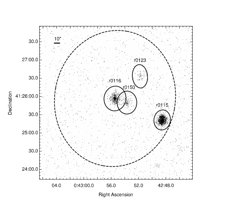
Figure 2: Source (solid ellipses) and background (dashed ellipse) apertures for four sources in a crowded region of Chandra OBSID 1575, from data obtained from Release 1.1 of the Chandra Source Catalog (Evans et al., 2010). Source aperture labels correspond to the Region IDs described in Table Determining X-Ray Source Intensity and Confidence Bounds in Crowded Fields. Data within the source apertures are excluded from the background aperture.

Figure 6: Posterior distributions for the four sources in Figure 2, computed using informative priors. The red and blue curves are for the first and second halves of the data set, computed using non-informative priors, and the black curves are the posterior distributions for the second half, using informative priors derived from the red curves. Vertical dashed lines indicate the mode and 68% confidence bounds computed from the entire data set, using non-informative priors (see Figure 5).

Average fractional error in source intensity as a function of $log_{10}r$ and $\Delta$ for relative background $b$ of $0.001,\,0.01,\,$ and $0.100$, from top to bottom. Contours for fractional errors of $-0.05,\,0.05,\,0.1,\,0.5,$ and $5.0$ are indicated. Sampled values are indicated by crosses and the interpolated surface is displayed using a logarithmic colormap. a) Case 1: overlap area in source apertures is assigned to the aperture for Source 1. b) Case 2: overlap area is assigned to the aperture for Source 2.

Average fractional width of source intensity probability distributions (see Figure Determining X-Ray Source Intensity and Confidence Bounds in Crowded Fields for plot details). a) Case 1: overlap area in source apertures is assigned to the aperture for Source 1. b) Case 2: overlap area is assigned to the aperture for Source 2.

Average fractional errors, as in Figure Determining X-Ray Source Intensity and Confidence Bounds in Crowded Fields based on maximum-likelihood determinations for source intensities and errors (see Figure Determining X-Ray Source Intensity and Confidence Bounds in Crowded Fields for plot details). a) Case 1: overlap area in source apertures is assigned to the aperture for Source 1. b) Case 2: overlap area is assigned to the aperture for Source 2.

Average fractional width of source intensity probability distributions, based on maximum-likelihood determinations for source intensities and errors (see Figure Determining X-Ray Source Intensity and Confidence Bounds in Crowded Fields for plot details). a) Case 1: overlap area in source apertures is assigned to the aperture for Source 1. b) Case 2: overlap area is assigned to the aperture for Source 2.

Average fractional errors and widths of source intensity probability distributions, assuming source apertures used in Rel. 1.1 of the Chandra Source Catalog. a) Average fractional errors. b) Average fractional widths.

References

- Broos et al. (2010) Broos, P. S., Townsley, L. K., Feigelson, E. D., Getman, K. V., Bauer, F. E., & Garmire, G. P., 2010, ApJ, 714, 1582
- Carter et al. (2003) Carter, C., Karovska, M., Jerius, D., Glotfelty, K., & Beikman, S., 2003, in Astronomical Data Analysis Software and Systems XII, ed. H. E. Payne, R. I. Jedrzejewski, & R. N. Hook, Vol. 295, 477
- Evans et al. (2010) Evans, I. N., et al., 2010, ApJS, 189, 37
- Freeman, Doe & Siemiginowska (2001) Freeman, P., Doe, S., & Siemiginowska, A., 2001, in Society of Photo-Optical Instrumentation Engineers (SPIE) Conference Series, ed. J.-L. Starck, F. D. Murtagh, Vol. 4477, 76
- Fruscione et al. (2006) Fruscione, A., et al., 2006, in Society of Photo-Optical Instrumentation Engineers (SPIE) Conference Series, Vol. 6270
- Jerius et al. (2004) Jerius, D. H., et al., 2004, in Society of Photo-Optical Instrumentation Engineers (SPIE) Conference Series, ed. K. A. Flanagan, O. H. W. Siegmund, Vol. 5165, 402
- Kashyap et al. (1994) Kashyap, V., Micela, G., Sciortino, S., Harnden, Jr., F. R., & Rosner, R., 1994, in The Soft X-ray Cosmos, ed. E. M. Schlegel, R. Petre, Vol. 313, 239
- Kashyap et al. (2010) Kashyap, V. L., van Dyk, D. A., Connors, A., Freeman, P. E., Siemiginowska, A., Xu, J., & Zezas, A., 2010, ApJ, 719, 900
- Kraft, Burrows & Nousek (1991) Kraft, R. P., Burrows, D. N., & Nousek, J. A., 1991, ApJ, 374, 344
- Laird et al. (2009) Laird, E. S., et al., 2009, ApJS, 180, 102
- Loredo & Wasserman (1993) Loredo, T., & Wasserman, I., 1993, in American Institute of Physics Conference Series, ed. M. Friedlander, N. Gehrels, & D. J. Macomb, Vol. 280, 749
- Loredo (1992) Loredo, T. J., 1992, in Statistical Challenges in Modern Astronomy, ed. E. D. Feigelson & G. J. Babu, 275
- Park et al. (2006) Park, T., Kashyap, V. L., Siemiginowska, A., van Dyk, D. A., Zezas, A., Heinke, C., & Wargelin, B. J., 2006, ApJ, 652, 610
- Raiffa & Schlaifer (1961) Raiffa, H., & Schlaifer, R., 1961, Applied Statistical Decision Theory, (Cambridge, Mass.: M.I.T. Press), first edition
- Stetson (1987) Stetson, P. B., 1987, PASP, 99, 191
- van Dyk et al. (2001) van Dyk, D. A., Connors, A., Kashyap, V. L., & Siemiginowska, A., 2001, ApJ, 548, 224
- Weisskopf et al. (2007) Weisskopf, M. C., Wu, K., Trimble, V., O’Dell, S. L., Elsner, R. F., Zavlin, V. E., & Kouveliotou, C., 2007, ApJ, 657, 1026