Novel energy detection using uniform noise distribution
Abstract
Energy detection is widely used in cognitive radio due to its low complexity. One fundamental challenge is that its performance degrades in the presence of noise uncertainty, which inevitably occurs in practical implementations. In this work, three novel detectors based on uniformly distributed noise uncertainty as the worst-case scenario are proposed. Numerical results show that the new detectors outperform the conventional energy detector with considerable performance gains.
Index Terms:
Average likelihood ratio test; cognitive radio; energy detection; noise uncertaintyI Introduction
Cognitive radio is considered to be a solution to the problems of spectrum under-utilization and “spectrum scarcity” [1]. The IEEE 802.22 Working Group has developed a standard for wireless regional area networks (WRAN) based on cognitive radio, which can operate on unused digital TV broadcast bands. In order to avoid interfering the primary services, the main task of WRAN is to detect the presence of the primary users. Many spectrum sensing methods have been proposed in the literature which can be mainly divided into three types: energy detection [2], matched-filter detection [3] and feature detection [4]. Among them, energy detection does not need any information about the primary signals and is widely used due to its simplicity [2]. Most works on energy detection assume that the noise power is accurately known. In reality, it is very difficult to obtain the accurate value of the noise power, leading to noise uncertainty [5]. The noise uncertainty can severely degrade the performance of energy detection [6].
In this work, three new energy detection schemes are proposed by using the distribution of the noise power in energy detection to remove the need for the noise power in the detector such that noise uncertainty can be avoided and energy detection can be improved. To do this, uniformly distributed noise power is adopted as the worst-case scenario, as the value of the noise power is equally likely across a certain interval. This uniform distribution is for noise power, not for noise uncertainty.
Numerical results show that the proposed new schemes have better performances than the conventional energy detector with noise uncertainty. They also show that even when there is a mismatch between the assumed uniform distribution and the actual distribution of the noise power, the new schemes still have considerable performance gains, verifying the robustness of the new schemes. Although the average likelihood ratio test (ALRT) [7] is not a new method and has been applied in many other works, the detectors from it are new and represent novelty. Due to the limited space, only the most relevant references on ALRT are discussed here, although there are other less relevant references on feature detectors.
II System Model
Consider the binary hypothesis testing problem for energy detection as
| (1) |
where represents the hypothesis that the signal is absent, indicates the hypothesis that the signal is present, index the signal samples, is the Gaussian signal with mean zero and variance [3, pp. 142], and is the additive white Gaussian noise with mean zero and variance . This assumption of Gaussian signal is widely used in previous works [3]. The Neyman-Pearson (NP) rule is commonly used. The performance of NP detection is measured by the pair of the detection probability and the false alarm probability . Similar to [2]-[4], this work does not consider the traffic load, which is the case when the primary user has very light traffic.
From (1), one can get the probability density function (PDF) of under as
| (2) |
and the PDF of under as
| (3) |
Then, ) under and ) under . The likelihood ratio test can be constructed according to [3, eq. (5.1)] as
| (4) |
where is the detection threshold and
| (5) |
| (6) |
Thus, one has from (4)
| (7) |
Denote the false alarm probability as
| (8) |
and the detection probability as
| (9) |
Therefore, the threshold can be determined as [3, pp. 143]
| (10) |
where is the right-tail probability for a random variable with degrees of freedom and is the inverse function of . This detector requires knowledge of the noise power in order to calculate the detection threshold. In practice, has to be estimated and the estimation error is random [6]. As a result, the estimate of used in the detection is also a random variable. This noise uncertainty leads to detection errors in (7). The proposed new detectors will not suffer from this estimation error and thus outperform (7).
Using the maximum likelihood method to estimate with samples, the PDF of the estimate is [8]
| (11) |
where is the estimate of the noise power . Note that this estimator uses pilot symbols in the training period of the secondary user. Such pilot symbols are not available from the primary user for spectrum sensing and thus, matched-filter detection cannot be used. Denote the detector in (7) as the NP-LRT detector, which is the conventional energy detector using the maximum likelihood estimate of the noise power.
One way of avoiding the noise uncertainty in (7) is to remove the use of in the detection. This can be achieved by averaging the likelihood function or the likelihood ratio over the distribution of based on the ALRT principle. References [9] and [10] analyzed the detector performance by averaging and . They did not average the decision variable to eliminate the noise uncertainty. We assume that is uniformly distributed over a certain interval as , with the PDF of
| (12) |
Uniform distribution has been widely used as a universal non-informative prior in many applications [11], especially when the parameter space is finite but the value and the distribution are unknown [12]. Compared with other distributions, such as log-normal distribution, the PDF of the uniform distribution has a simple structure and therefore closed-form energy detectors can be derived. Also, uniform distribution can be regarded as the worst-case scenario because the noise power is equally likely anywhere in the whole interval [13]. Thus, this is a very useful benchmark. In reality, the noise power equals , where is the single-sided power spectral density and is the bandwidth. Further, where is the Boltzman constant and is the temperature. Thus, as long as is fixed and is uniformly distributed over a certain interval with limited low temperature and high temperature, the noise power is also uniformly distributed in this case. Most receivers do have an operating range of temperature, which can be used to determine and together with and . Note that in realistic situation, one also needs to consider electrical and thermal noise, frequency response and other factors, but to simplify the detector, this work only considers the ideal situation where . In the realistic situation, one can assume the noise power equals , where is a constant which takes electrical noise, frequency influence and other factors into account.
III New energy detectors
In this section, three new detectors based on the uniform distribution of are proposed. The first one is denoted as NP-AVE detector which averages the likelihood function of each sample over the uniform distribution of . The second one is denoted as NP-AVN detector which averages the overall likelihood function of all the samples over the uniform distribution of . It is very difficult to obtain the exact average likelihood ratio over the uniform distribution of . Thus, this work conducts averaging over the numerator and the denominator separately to obtain tractable approximate detectors. This is somewhat brute-forced but still useful. The third one is denoted as the NP-LLR detector, which is obtained by averaging the log-likelihood ratio over the distribution of . Note that there are no closed-form expressions of and for the NP-AVE and NP-AVN detectors and one has to calculate them by numerical integrations. For the NP-LLR detector, the closed-form expression is available and will be provided.
III-A NP-AVE detector
One can get NP-AVE detector as
| (13) |
where is the detection threshold and
| (14) | ||||
and
| (15) | ||||
Proof: See Appendix. .
Due to the complexity of the decision variable in (13), the detection threshold will be calculated by simulation.
III-B NP-AVN detector
The NP-AVN detector is derived as
| (16) | ||||
where the exponential integral function [14] and is the detection threshold of the NP-AVN detector.
Proof: See Appendix. .
Again, due to the complicated structure of the decision variable in (16), has to be calculated via simulation.
III-C NP-LLR detector
Proof: See Appendix. .
Using (18), the detection threshold can be determined as
| (20) |
where is the inverse function of with parameters and . Denote the detector in (17) as Neyman-Pearson log-likelihood ratio (NP-LLR) detector. The receiver operating characteristic (ROC) curve for NP-LLR detector can be easily obtained using (20) in (19). Note that (17) has the same decision variable as the conventional detector in (7). However, the detection threshold in (7) depends on the noise power and thus suffers from noise uncertainty, while the detection threshold in (20) is independent of noise power such that (17) does not have noise uncertainty. Thus, they are different. Note that the new detectors do use the extra knowledge of the interval and the distribution of the noise power. This can be considered as a stochastic maximum likelihood method when the unknown parameter is eliminated by averaging over its distribution. The values of and are easier to obtain than , as they are only determined by the upper and lower limits of the possible range of . In practice, they can be calculated from the operating range of the receiver temperature when the bandwidth is fixed. Note also that all the detectors are compared based on the assumption of independent samples. This assumption has been widely used in the literature [15]. For the noise samples, this can be achieved by Nyquist sampling. For the signal samples, this can be achieved when the Doppler shift is large or the sampling interval is large.
IV Numerical results and discussion
In this section, the performances of the conventional detector with the maximum likelihood estimate given in Section 2 and the three new detectors derived in Section 3 are evaluated via computer simulation. Define the received signal power as and assume that the noise power is uniformly distributed over the interval . Define . In all the figures, “NP-LRT” refers to the conventional detector in (7), “NP-AVE” refers to the new detector in (13), “NP-AVN” corresponds to the new detector in (16) and “NP-LLR” refers to the new detector in (17). The thresholds and are calculated from Monte Carlo trials using the NP rule while the threshold and the threshold are calculated by (10) and (20), respectively. Also, assume that the bandwidth is and , together with the Boltzmann constant . Then, the noise power of , , , in the simulation below correspond to the temperature of 150K, 210K, 391K, 451K, respectively.
Fig. 1 compares the ROC curves for the NP-AVN, NP-AVE, NP-LLR and NP-LRT using maximum likelihood estimate with or at and . Fig. 1(a) considers the noise interval as = 0.7 and = 1.3 while Fig. 1(b) enlarges the noise interval to = 0.5 and = 1.5. One can see that the performances of these four detectors degrade when the noise interval increases, as expected. On the other hand, the performance gains of the new detectors over the conventional detector are large but decrease when the noise interval increases.
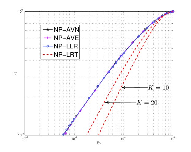
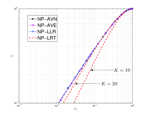
Fig. 2 compares the ROC curves for the NP-AVN, NP-AVE, NP-LLR and NP-LRT with or at , = 0.5 and = 1.5 for different . One can see that the performance gains of these new detectors increase when the received signal power increases. Also, one can see from Fig. 1(b) and Fig. 2(a) that the performance gains of the new detectors over the conventional detector increase when increases. The performance gains of the new detectors over the conventional detector are still substantial even at low SNRs.
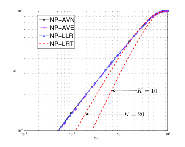
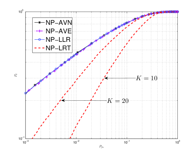
Fig. 3 compares the ROC curves for the NP-AVN, NP-AVE, NP-LLR and NP-LRT at and when the noise power follows a log-normal distribution with variance and the uniform distribution in the interval between and . Fig. 3 (a) considers while Fig. 3 (b) reduce the variance to . These figures are used to examine the effect of mismatch between assumed and actual noise power distributions on the performances of the new detectors, as the simulated samples are generated using log-normal distribution while the derivation in Section 3 assumes a uniform distribution. One can see that the three new detectors based on the uniform distribution still have considerable gains over the conventional detector even when the actual noise power follows a log-normal distribution. Moreover in Fig. 3 (a), one can see that the performances of the new detectors do degrade for small values of when there is a mismatch. However the performance degradation is quite small compared to their performance gains over the conventional detector. On the other hand, when the variance of log-normal distribution decreases, the gain of our new detectors over the conventional one increases.
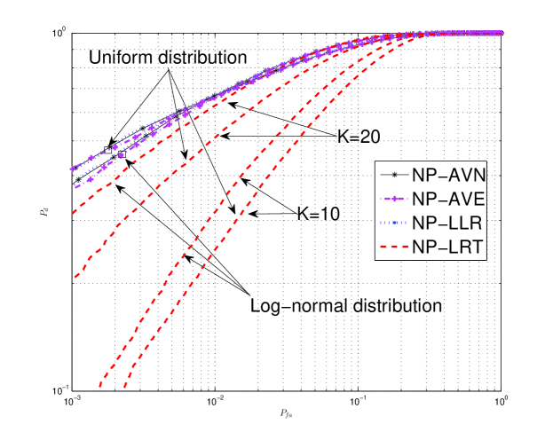
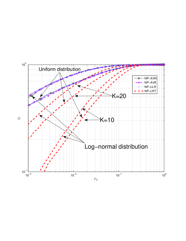
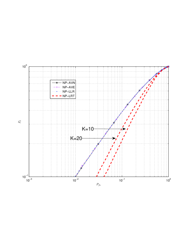
Fig. 4 compares the ROC curves for the NP-AVN, NP-AVE, NP-LLR and NP-LRT at , , and when the interference is assumed to follow a normal distribution with variance . This figure is used to examine the performances of new detectors over the conventional detector when the interference exists. Comparing Fig. 4 with Fig. 1 (a), one can see that, although the performances of new detectors degrade, there is still considerable gain of the new detectors over the conventional one in Fig. 4. Therefore, our new detectors are still useful even when interference exists.
As expected, one can see from these figures that the performance of NP-LRT detector improves when the number of samples increases. Also, one can find the NP-LLR detector gives the best detection performance while the conventional NP-LRT detector has the worst performance. Although the NP-AVN, NP-AVE and NP-LLR detectors have very close performances, they have different structures and complexities. NP-AVN detector has a slightly better performance but a more complicated structure than the NP-AVE detector because it includes exponential integral function. Specifically, NP-AVN detector takes 0.54 seconds while NP-AVE detector only takes 0.001 seconds in Matlab R2013a simulation using a computer with 64-bit operation system, CPU i7-2600 and 4G memory. Moreover, the NP-LLR detector has closed-form expressions for the threshold, the detection probability and the false alarm probability. Thus, one can choose the suitable detector according to their application for different performances or complexities. We have also found that the NP-AVN detector is more robust than NP-AVE detector to the mismatch between the assumed noise power interval and the true noise power interval.
V Conclusion
New energy detectors based on the uniform distribution of the noise power have been proposed. Numerical results have shown that these new detectors outperform the conventional detector in the presence of noise uncertainty. The performance gain depends on the received signal power, the noise power interval and the number of samples. This gain is achieved by using the extra knowledge of the uniform distribution and comparison of these detectors reveals the effect of this extra knowledge and therefore is useful. The new detectors however have similar performances, as can be seen from the figures.
APPENDIX A: DERIVATION OF THE NP-AVE DETECTOR
APPENDIX B: DERIVATION OF THE NP-AVN DETECTOR
APPENDIX C: DERIVATION OF THE NP-LLR DETECTOR
References
- [1] S. Haykin, “Cognitive radio: brain-empowered wireless communications,” IEEE Journal on Selected Areas in Communications, vol. 23, no. 2, pp. 201–220, Feb. 2005.
- [2] H. Urkowitz, “Energy detection of unknown deterministic signals,” Proceedings of the IEEE, vol. 55, no. 4, pp. 523–531, Apr. 1967.
- [3] S. M. Kay, Fundamentals of Statistical Signal Processing: Detection Theory. Prentice-Hall, 1998.
- [4] D. Cabric, S. M. Mishra, and R. W. Brodersen, “Implementation issues in spectrum sensing for cognitive radios,” in Conference Record of the Thirty-Eighth Asilomar Conference on Signals, Systems and Computers, vol. 1, Nov. 2004, pp. 772–776.
- [5] A. Sonnenschein and P. Fishman, “Radiometric detection of spread-spectrum signals in noise of uncertain power,” IEEE Transactions on Aerospace and Electronic Systems, vol. 28, no. 3, pp. 654–660, July 1992.
- [6] R. Tandra and A. Sahai, “SNR Walls for signal detection,” IEEE Journal of Selected Topics in Signal Processing, vol. 2, no. 1, pp. 4–17, Feb. 2008.
- [7] P. Panagiotou, A. Anastasopoulos, and A. Polydoros, “Likelihood ratio tests for modulation classification,” in 21st Century Military Communications Conference Proceedings (MILCOM 2000), vol. 2, 2000, pp. 670–674.
- [8] Y. Chen and N. C. Beaulieu, “Maximum likelihood estimation of snr using digitally modulated signals,” IEEE Transactions on Wireless Communications, vol. 6, no. 1, pp. 210 –219, Jan. 2007.
- [9] D. Chen, J. Li, and J. Ma, “Cooperative spectrum sensing under noise uncertainty in cognitive radio,” in 4th International Conference on Wireless Communications, Networking and Mobile Computing, 2008, pp. 1–4.
- [10] H. Wang, Y. Xu, X. Su, and J. Wang, “Cooperative spectrum sensing in cognitive radio under noise uncertainty,” in Proc. of 71st IEEE Vehicular Technology Conf., May 2010, pp. 1–5.
- [11] N. Shulman and M. Feder, “The uniform distribution as a universal prior,” IEEE Transactions on Information Theory, vol. 50, no. 6, pp. 1356 – 1362, June 2004.
- [12] H. Jeffreys, “An invariant form for the prior probability in estimation problems,” Proceedings of the Royal Society of London. Series A, Mathematical and Physical, vol. 186, no. 1007, pp. 453–461, Sep. 1946.
- [13] E.-W. Bai, R. Tempo, and M. Fu, “Worst-case properties of the uniform distribution and randomized algorithms for robustness analysis,” Mathemtics of Control, Signals and Systems, vol. 11, no. 3, pp. 183–196, 1998.
- [14] D. M. Smith, “Multiple-precision exponential integral and related functions,” ACM Transactions on Mathematical Software, vol. 37, no. 4, pp. 1 – 16, Feb. 2011.
- [15] G. L. Stüber, Principles of Mobile Communication, 3rd ed. Springer, 2012.
- [16] I. S. Gradshteyn and I. M. Ryzhik, Table of Integrals, Series, and Products, 6th ed. San Diego, CA: Academic, 2000.