Anomalous transport of subdiffusing cargos by single kinesin motors: the role of mechanochemical coupling and anharmonicity of tether
Abstract
Here we generalize our previous model of molecular motors trafficking subdiffusing cargos in viscoelastic cytosol by (i) including mechanochemical coupling between cyclic conformational fluctuations of the motor protein driven by the reaction of ATP hydrolysis and its translational motion within the simplest two-state model of hand-over-hand motion of kinesin, and also (ii) by taking into account the anharmonicity of the tether between the motor and cargo (its maximally possible extension length). It is shown that the major earlier results such as occurrence of normal versus anomalous transport depending on the amplitude of binding potential, cargo size and the motor turnover frequency not only survive in this more realistic model, but the results also look very similar for the correspondingly adjusted parameters. However, this more realistic model displays a substantially larger thermodynamic efficiency due to a bidirectional mechanochemical coupling. For realistic parameters, the maximal thermodynamic efficiency can be transiently about 50% as observed for kinesins, and even larger, surprisingly also in a novel strongly anomalous (sub)transport regime, where the motor enzymatic turnovers become also anomalously slow and cannot be characterized by a turnover rate. Here anomalously slow dynamics of the cargo enforces anomalously slow cyclic kinetics of the motor protein.
pacs:
05.40.-a,87.10.Mn,87.16.Uv,87.16.Nn1 Introduction
The problem of how molecular motors can operate and realize transport in such a crowded environment as cytosol of biological cells [1, 2, 3] came only recently in the limelight of attention [4, 5, 6, 7, 8, 9, 10, 11, 12]. Indeed, numerous recent experiments reveal that submicron particles like various endosomes and organelles, mRNA molecules, ionic channels and even smaller nanoparticles diffuse passively anomalously slow with mean-square distance growing sublinearly in time rather than simply diffuse (linear growth) on the relevant mesoscopic time and spatial scales [4, 6, 13, 14, 15, 16, 17, 18, 19, 20, 21, 22, 23, 24, 25, 26, 27, 28, 29, 30]. Molecular motors such as various kinesins are thus indispensable for delivering such and similar cargos e.g. along axons of neuronal cells [31]. In a two-state flashing ratchet model of molecular motors with position-independent switching rates it has been shown that a power stroke like operation mechanism can perfectly overcome subdiffusion slowness and result into a highly efficient normal transport characterized by mean transport velocity [10, 11]. However, the very possibility to realize such a normal active transport of (passively) subdiffusing cargos presents a highly nontrivial issue. It depends on (i) the binding strength of motor protein to the microtubule providing a transport highway, (ii) cargo size, (iii) motor operating frequency, (iv) external force directed again the processive motion of the motor [10, 11], and (v) the strength of the tether or linker connecting the motor and its cargo [11]. Anomalous active transport can also be typical for living cells [10, 11], and indeed an increasing number of experiments reveals its occurrence [17, 6, 30]. Our modeling route is based on non-Markovian Generalized Langevin Equation (GLE) [32, 33] description of viscoelasticity [34, 35, 36, 37] and its multi-dimensional Markovian embedding [36, 37]. The approach is deeply rooted in the main principles and dynamical foundation of statistical mechanics such as dynamical theory of Brownian motion and fluctuation-dissipation theorem [32, 33], which must hold when the system is at thermal equilibrium. The approach explains the dynamical origin of both normal and anomalous Brownian motion and naturally extends beyond thermal equilibrium, which makes it most suitable to describe physical processes in living cells. Our theory naturally explains, in particular, why the power exponent of anomalous active transport can be larger than one of the passive subdiffusion and why the power exponent of anomalous active Brownian motion can be larger than doubled exponent of passive motion [6, 30]. Such experimental facts cannot be consistently explained within the previous approaches [4, 7] to anomalous transport by molecular motors, as detailed in [11]. In fact, we develop a rather straightforward generalization of the Brownian ratchets approach to modeling of molecular motors [38, 39, 40, 41, 42, 43, 45, 46, 47, 48, 44], with a well proven utility in the case of molecular motors underlying memoryless Markovian dynamics, towards anomalous non-Markovian dynamics with long-lasting memory reflecting viscoelastic effects in cytosol. Non-Markovian dynamics can nevertheless be considered as low-dimensional projection of a multi-dimensional Markovian dynamics – the idea which has a long tradition in statistical mechanics [50].
As it is is well known, microtubule is a periodic electrically polar structure featured by asymmetric periodic distribution of negative and positive charge densities on its surface [1, 51]. It has a spatial period nm. Furthermore, the charge state of the motor protein depends on whether it is nucleotide free (no extra charges are present), either ATP, or ADP and the phosphate group are bound (three extra negative elementary charges altogether in each case), or only ADP is bound (two extra negative elementary charges). Reflecting the change of charge distribution on the motor protein the motor binding potential in the electrical field of microtubule can also change accordingly [41]. Being periodic in space it should, however, be spatially asymmetric, and this asymmetry can direct molecular motor in one selected direction (which can depend on the particular kind of motor) when the binding potential begins to stochastically fluctuate. These fluctuations can be caused by changing the overall charge of the motor protein accompanied by its conformational fluctuations due to the reactions of ATP binding, hydrolysis and dissociation of the products, repeated cyclically at random time instances. For two-headed kinesin molecules, one of the simplest, minimal model assumptions is to assume just two realizations of the binding potential depending on the motor state with the additional symmetry (the heads are assumed to be identical and treated on equal footing) [39, 40, 41, 42, 43, 46] . This ensures that two subsequent half-steps of the equal length makes one total step in the direction defined by the asymmetry of the potential, see in Fig. 1. Kinesins consume one ATP molecule per one full step. Hence, energy eV is invested into a half-step. Simplest further assumption is to characterize the switching process by one spatially-independent rate , so that the averaged motor turnover frequency is . A shortcoming of this approach is that it does not specify a mechanism of how the energy of ATP hydrolysis is invested into the change of . Neither reflects it the back influence (i.e. the mutual coupling) of the mechanical motion along microtubule on the biochemical turnovers of the motor enzyme. In particular, it is not consistent with the demand that if to gradually bring the reaction of ATP hydrolysis to thermodynamic equilibrium, , the translation motion of molecular motor must also gradually vanish. Nevertheless, this ratchet approach remains immensely popular for Markovian dynamics [44, 45, 40, 46, 48]. It has been generalized for anomalously operating motors in Refs. [10, 11]. The role of mechanochemical coupling [44, 39, 43, 40, 49] is, however, important to address. In the present work, we consider a simplest popular model of kinesins with spatially- and -dependent transition rates reflecting a mechanochemical coupling of the translation motion of motor protein and its conformational cyclic dynamics. We also consider an anharmonic model for tether connecting the motor and cargo by taking into account its maximally possible extension length, which encompasses the previous harmonic model [11] as a limiting case used for comparison.
2 The model and methods

We start from considering subdiffusive overdamped 1d dynamics of cargo with radius and coordinate subjected to both viscous Stokes friction with friction coefficient and memory friction with kernel , as well as to unbiased Gaussian thermal random forces and of the environment at temperature which are completely characterized by their autocorrelation functions
| (1) | |||
| (2) |
The above relations express the second (classical) fluctuation-dissipation theorem (FDT) by Kubo [32, 33]. It has a very important physical content. Namely, at the thermal equilibrium the energy loss due to friction is completely compensated by the energy gain from thermal stochastic force serving as a “stochastic lubricant”. Without it the motion would stop due to frictional losses. However, beyond thermal equilibrium there emerges an overall heat flux to the environment, even in the absence of a temperature gradient. Minimizing this flux one can arrive at the best thermodynamic efficiency of transport. This is a very important point: there is no need to minimize the friction, contrary to a popular belief, but rather try to stay most closely to the thermal equilibrium, in order to minimize the heat losses. Furthermore, the cargo is coupled to the motor with coordinate by an elastic tether or linker for which we use a finitely extensible non-linear elastic (FENE) model [52] with coupling energy
| (3) |
where , and is elastic coupling constant. For a small extension, , , recovering harmonic spring model, and the maximal extention length is . The motor is also characterized by Stokes friction and the corresponding thermal force obeying FDT (1) with . It moves in the binding potential which depends on the motor conformation . Altogether,
| (4) | |||||
| (5) |
where is an external loading force applied directly to the motor (for harmonic linker, , it is the same as to apply it to the cargo).
If the cargo is not coupled to the motor (), the fractional memory friction , , with fractional friction coefficient leads to subdiffusion of cargo, , at the sufficiently large times . Subdiffusion is characterized by the fractional diffusion coefficient . Initially, for diffusion is, however, normal with . For all times in this model [53],
| (6) |
where is the generalized Mittag-Leffler function. For the coupled motor and cargo, in the limit of infinitely rigid harmonic linker , one can exclude explicitely (see discussion in Ref. [11]) the cargo dynamics and consider anomalous dynamics of the motor alone, characterized by the Stokes friction , and the same memory friction. This would provide a generalization of the model studied in Ref. [10]. We consider here but a more general model.
For the binding potential, we consider the same model of piecewise linear asymmetric potential with amplitude , spatial period , and the maximum dividing the spatial period in the ratio , with , as in Ref. [11], see in Fig. 1. Similar models are well-known and widely used [41, 42].

Important distinction between different further models possible occurs on the level of intrinsic enzyme dynamics . The chemical coordinate must be cyclic, with the cycle driven preferably in one direction (rotation of “catalytic wheel” [54, 47]) by the free energy released from the reaction of ATP hydrolysis kept out of the thermodynamical equilibrium (shifted to the right) by maintaining out-of-equilibrium concentrations of reactants. One of simplest related cycles involves four discrete states (Fig. 2, left) [43]. The ratio of the product of the (pseudo-first order) rates (ATP, ADP, and molecules are abundant with concentrations kept constant) of the counter-clockwise transitions to the product of rates in the clockwise transitions must be equal [55, 56]. In the case of two-headed kinesins, it should be applied to each head, with the rates which are position-dependent (mechano-chemical coupling) which would make already a rather complicate model. The simplest possible drastical reduction accounting for the mechano-chemical coupling in the case of head-over-head motion of kinesins, a so-called two-state cycle [55, 43, 40], is shown in the right part of Fig. 2. One considers only two states and two realizations of obeying additional symmetry , with each transition accounting for a half-step (one head moves, another remains bound). The corresponding rates must be not only periodic in space, , , but also share additional symmetries, and . For a two-cycle it also must be:
| (7) |
for any , which can be satisfied, e.g., by choosing
| (8) |
The total rates
| (9) |
of the transitions between two energy profiles must satisfy
| (10) |
at thermal equilibrium (thermal detailed balance condition of vanishing dissipative fluxes both in the translation direction and within the conformational space of motor) [39, 40]. It is obviously satisfied for , where both the flux in the transport direction and the flux within the chemical coordinate space vanish together. Notice that if to choose , the latter condition is not possible to satisfy.
We still have some freedom in choosing various models for or . The rate corresponds to the reactions of ATP binding and hydrolysis considered as one lump reaction. It is reasonable to assume that this rate is constant, within some neighborhood of the minimum of potential and is zero otherwise. Correspondingly, the rate within neighborhood of the minimum of potential . Given these assumptions we have:
| (11) |
Furthermore, if we choose (for the given model of binding potential with ), then ATP binding to the motor and its hydrolysis can occur, in principle, anywhere on microtubule with the same rate. This is a reasonable assumption from the biophysical point of view, which lends a further support for our model choice. It is easy to grasp that this model can give very similar results to the ratchet model with spatially independent rates [11] for sufficiently large and potential amplitude having similar values. Then, is approximately the motor turnover frequency which is nearly independent of . This provides a possibility to compare the studied model with the model in Ref. [11] by choosing other parameters appropriately.
2.1 Energetics of the motor
In Eqs. (4), (5), , , describe total environmental forces. The averaged work done by these forces, , , is nothing else as the total heat exchange with the environment, . At thermal equilibrium, , i.e. overall heat exchange is absent. Beyond thermal equilibrium, describes the heat transfer to the environment or heat losses. The averaged energy transduced by the potential flashes is [57], which yields the averaged sum of the binding potential jumps at the transition points . The mechanical work done by the motor against the external load is . The energy balance is , if to neglect the back coupling of the potential fluctuations to the biochemical cycle of the motor, i.e. the energy transferred back to the motor and the ATP energy source, which drives the whole machinery. Hence, thermodynamic efficiency within such a treatment is
| (12) |
It becomes constant for a sufficiently large , in the case of normal transport, where both , and , but algebraically decays to zero, , in the case of anomalous transport, , in the cases of a periodic potential modulation [58, 53], or constant potential-independent flashing rates [10, 11]. In the absence of external load, , , i.e. all the input energy is eventually dissipated as heat. However, something useful is yet done. Namely, the cargo is transferred on some distance . Different Stokes efficiencies have been defined to characterize energetic performance of motors in such a situation for memoryless friction [59, 60, 61]. However, the notion of Stokes efficiency becomes even more ambiguous for viscoelastic environment [53]. For this reason, a delivery efficiency has been introduced in Ref. [10]. It is the ratio of the mean velocity of the cargo delivery to the mean number of motor enzyme turnovers made,
| (13) |
The definition (12) is the only possibility to define thermodynamic efficiency in the case of ratchet models which do not specify the mechanism of mechanochemical coupling. Within these models, is considered as a driver which provides input energy unidirectionally, i.e. without feeling any feedback [57]. However, within the considered model with a mutual coupling of the conformational cycling of the motor enzyme and its translational motion the interaction energy provides a bidirectional coupling. The energy can flow in both directions. The energy supply is provided by a pool of ATP molecules which is characterized by out-of-equilibrium chemical potential difference of the reaction of ATP hydrolysis, which we denoted as . Hence, it is reasonable to define the input energy as [39]. Then, the thermodynamic efficiency is
| (14) |
The idea is clear: each turnover of the catalytic wheel requires energy of the hydrolysis of one ATP molecule, in accordance with the main principles of the non-equilibrium thermodynamics applied to the biochemical cycle kinetics [55, 56]. One expects that . This is because a part of the energy can be given back to the motor, its intrinsic degree of freedom, and e.g. recuperated in the backward synthesis, . This feature is beyond simple ratchet models with spatially independent rates which do not take properly into account such a mechano-chemical coupling. However, this definition is also not quite precise. As a matter of fact, one ATP molecule is only consumed if a cycle is accomplished in the counter-clockwise direction in the left diagram of Fig. 2. Moreover, it is recuperated if the cycle is completed in the clockwise direction. Therefore, for the two-state cycle depicted in the right diagram of Fig. 2, to correctly calculate consumption of ATP molecules we should count , with for the transition , and with for the transition . The correspondingly calculated input energy is denoted as , and thermodynamic efficiency as . Obviously, since , . However, in a regime, where the catalytic wheel rotates overwhelmingly in one direction (like in Michaelis-Menthen treatment of enzymatic reactions, where the backward rotation is entirely neglected), the distinction between and becomes negligible. By the same token, one can modify the definition of the delivery efficiency in Eq. (13) by replacing with the averaged number of ATP molecules hydrolyzed. However, the difference between both definitions exists only beyond the Michaelis-Menthen description of the motor kinetics.
2.2 Markovian embedding and numerical method
Following to already well-established methodology of Markovian embedding of Refs. [36, 5, 37] we approximate power-law memory kernel by a sum of exponentials,
| (15) |
obeying fractal scaling , , and introduce auxiliary Brownian particles modeling viscoelastic properties of the environment. This allows to transform the considered non-Markovian problem into a Markovian problem in the space of enhanced (by ) dimensionality. Then, the standard methods of integration stochastic differential equations (SDEs), such as stochastic Euler, or stochastic Heun method, can be applied for a fixed realization of the potential . The method allows for a highly accurate numerical integration of fractional Langevin dynamics even for a moderate [36]. The accuracy of kernel approximation is controlled by the scaling parameter and even for the decade scaling expressing the idea “one power law time decade requires about one exponential in doing approximation” it is better than 4% between two memory cutoffs, short time cutoff , and large time cutoff . For , the accuracy of approximation improves to about [58]. Statistical errors in numerical simulations due to a finite number of trajectory realizations will always be larger for a practical , scaling as . For , suffices for most practical purposes with the accuracy of several percents which in stochastic simulations is considered as a very good one. Given the maximal time range of subdiffusion defined by , one can always find appropriate minimal Markovian embedding with the required accuracy. Since this ensures excellent numerical method [36, 37]. The finiteness of reflects finite effective viscosity of cytosol fluid which can be exponentially enhanced with respect to one of water depending on the cargo size [62, 63, 64]. Indeed, the effective friction at very large times is and on the scaling grounds, . For , passive diffusion of cargo becomes again normal. It is characterized by the friction coefficient and diffusion coefficient largely suppressed with respect to water. With these parameters [10],
| (16) |
Following to [37, 11], upon introduction of auxiliary overdamped Brownian particles with coordinates and frictional coefficients , the Markovian embedding dynamics reads
| (17) |
where , and . Furthermore, are uncorrelated white Gaussian noises of unit intensity, , which are also uncorrelated with the white Gaussian noise sources and . To have a complete equivalence with the stated GLE model in Eqs. (4), (5) with memory kernel (15), the initial positions are sampled from a Gaussian distribution centered around , with variances [37].
2.2.1 Choice of parameters and details of numerics.
As in Ref. [11], we take nm for the effective radius of kinesin, about 10 times larger than its linear geometrical size (without tether) in order to account for the enhanced effective viscosity experienced by the motor in the cytosol compared to its value in water. The viscous friction coefficient is estimated from the Stokes formula as , where is water viscosity. Furthermore, we use the characteristic time scale to scale time in the numerical simulations with . For the above parameters, . Distance is scaled in units of , elastic coupling constants in units of pN/nm, and forces in units of pN. was chosen ( 1/s) yielding ns, and was as found experimentally in [6, 21]. Two cargo sizes were considered, large nm, which corresponds to the magnetosome size in Ref. [6], and a smaller one. For larger cargo, we assume that its effective Stokes friction is enhanced by the factor of in cytosol. Assuming that s this yields fractional friction coefficient with [11], which yields subdiffusion coefficient . It is in a semi-quantitative agreement with the experimental results in [6]. Smaller cargo is characterized by yielding , ten times larger. Furthermore, we used two values of rate constant : (fast) and (slow), in order to match approximately the enzyme turnover rates in Ref. [11]. Accordingly, we used mostly in simulations, although we used also two larger values of , see Table 1, in order to arrive at the thermodynamical efficiencies as large as 50% typical for kinesins [44]. Moreover, two different values for the elastic spring constant were used, pN/nm (‘strong’), which corresponds to measurements in vitro [65], and a ten times softer spring pN/nm (‘weak’), in accordance with recent results in Ref. [21] in living cells. For the maximal extension of linker we used nm [1, 31], and also , which corresponds to harmonic linker in Ref. [11]. The studied set of parameters is shown in Table 1.
| Set | , | , pN/nm | , | , | , nm |
|---|---|---|---|---|---|
| 171 | 0.320 | 170 | 20 | ||
| 1710 | 0.320 | 170 | 20 | ||
| 1710 | 0.032 | 170 | 20 | ||
| 171 | 0.032 | 170 | 20 | ||
| 171 | 0.032 | 170 | 20 | 80 | |
| 171 | 0.320 | 34 | 20 | ||
| 171 | 0.032 | 34 | 20 | 80 | |
| 171 | 0.320 | 170 | 25 | 80 | |
| 171 | 0.320 | 170 | 30 | 80 | |
| 1710 | 0.320 | 170 | 25 | 80 | |
| 1710 | 0.320 | 170 | 30 | 80 |
In order to numerically integrate stochastic Langevin dynamics following to one potential realization , we used stochastic Heun method implemented in parallel on NVIDIA Kepler graphical processors. Stochastic switching between two potential realizations is realized using a well-known algorithm. Namely, if the motor is on the given surface or , at each integration time step it can switch with the probability or to another surface, or to evolve further on the same surface, where is the integration time step, and are given in Eq. (2). A particular embedding with and was chosen in accordance with our previous studies. Furthermore, we use and trajectories used for the ensemble averaging. The maximal time range of integration was , which corresponds to sec of motor operation. was taken in all numerical simulations. We also checked that with , the motor stops at , i.e. no directed motion and useful work can be derived from the reaction of ATP hydrolysis being at thermal equilibrium, in accordance with stochastic thermodynamics of isothermal engines [55, 56].
3 Results and Discussion
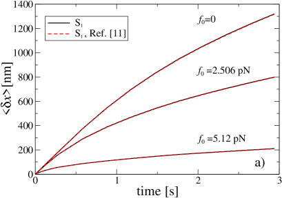
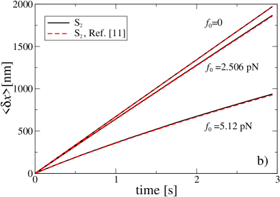
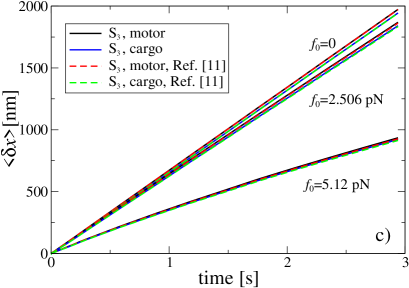
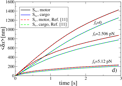
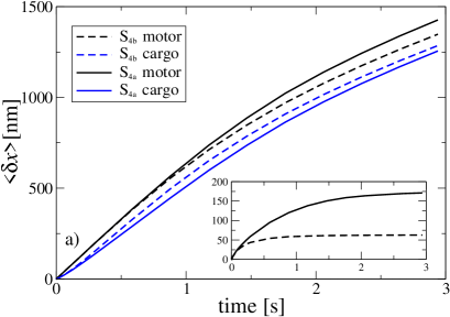
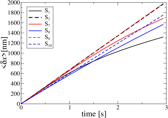
We compare first in Fig. 3 the results for the parameter sets , , , of the present model and the corresponding parameter sets , , , in Ref. [11] , for the ensemble averaged trajectories. One can see that almost no difference can be visually detected, both for larger and smaller cargo, stronger and weaker linker. The transport is clearly anomalously slow for and always (large cargo), and it changes from normal to anomalous transport upon increase of in the cases and (smaller cargo). For stronger linker, the difference between the motor and cargo positions is not significant, and for this reason the cargo position is not shown in Fig. 3, (a),(b). For weaker linker, the difference becomes very strong in the case of large cargo, see in Fig. 3, d, where for it increases up to about nm, see in the Fig. 4, a, inset. The corresponding elastic energy becomes , i.e. of the same of order as a typical energy of covalent bonds and such a linker clearly cannot sustain transport [11]. It will be disrupted. However, the linker anharmonicity starts to play a profound role when the cargo-motor distance becomes larger than about one fifth of the maximal linker extension . The latter one can be in the range between 10 nm and 150 nm for different motors [1, 31]. We consider nm (). Then, for a strong linker the anharmonicity does not play any essential role. We clarify its role in Fig. 4, a for a weak linker and large cargo. It is seen that anharmonicity restricts the increase of the cargo-motor distance by nm. Substituting this value in Eq. (3) yields . Such a linker should be able to sustain transport of large cargo, not necessarily it will be disrupted. This is an important result: Even weak linkers can possibly support strongly anomalous transport of large cargos due to nonlinear effects.
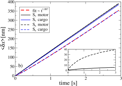
In Ref. [11], we revealed a very interesting effect which can emerge due to the weakness of linker. Namely, if to reduce the turnover frequency of motor pulling large cargo from 85 to Hz (which is the case in [11]) then the motor operates normally at , whereas the cargo enters temporally a super-transport regime with . A natural question emerges if this effect survives for the considered FENE model of linker. Fig. 4, b answers this question in affirmative, lending it therefore further support with respect to possible experimental verification. The explanation of this effect is simple: When the motor is in normal regime, its distance increases linearly in time. However, for a weak linker the retardation of the cargo past the motor increases sublinearly in time, see inset in Fig. 4, b. This causes the effect that the mean distance covered by cargo increases super-linearly in time, although it, in fact, moves slower than motor. Clearly, in this case “super”-transport does not imply a faster transport at all! The cargo lags behind the normally walking motor. Interestingly, sub-transport also does not proceed necessarily slower than the normal one [66, 67, 68].
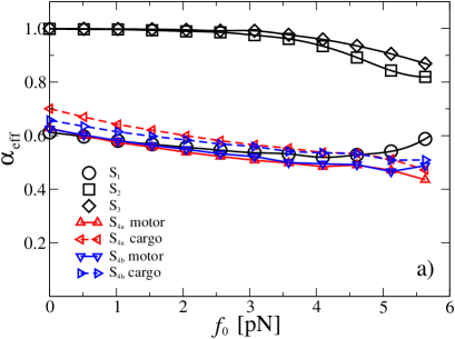
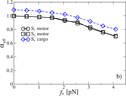
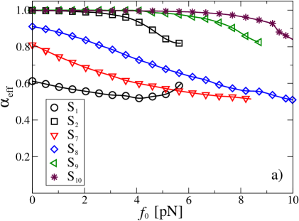
The effective transport exponents of motor and cargo (the latter one in some cases only, where the difference is substantial) are shown in Fig. 5. Their behavior is rather similar to one studied in [11]. The new feature is that the difference between for the motor and cargo in the case of the transport of large cargo on weaker linker becomes smaller due to nonlinear effects in elastic coupling. This is, however, what was to expect, not a surprise.
3.1 Thermodynamic efficiency
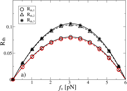
The real discrepancies between the studied model and the model in [11] appears only for the thermodynamic efficiency, see in Fig. 6. Indeed, is essentially larger than , and is slightly larger than . The latter relative discrepancy is, however, less than 2% for the set (strongly anomalous transport) and becomes almost negligible for the set (close to normal transport), indicating that “catalytic wheel” rotates overwhelmingly in one direction. Notice also that the difference between and the same quantity for similar parameter sets in Ref. [11] is small. This once more confirms that the ratchet models with constant, spatially independent rates provide a reasonable description of the work of molecular motors. What they, however, cannot do properly indeed is to describe thermodynamic efficiency of the motor. This is a principal shortcoming because simple ratchet models do not take properly the (bidirectional) mechano-chemical coupling into account. The correct definition of thermodynamic efficiency of molecular motors is one given by , and it can be essentially larger than .
However, the normal modus operandi of linear molecular motors such as kinesins is one at zero thermodynamic efficiency (). The work is done entirely on overcoming the dissipative resistance of the environment while relocating cargo from one place in the cell to another one. Neither potential energy of the motor, nor the potential energy of the cargo is enhanced at the end. This is very different from the work of the ionic pumps whose primary goal is to enhance the electrochemical potential of the pumped ions. The cargo delivery efficiency exhibits the same features revealed in Refs. [10, 11], and we do not consider it in further detail in this paper, referring the readers to Ref. [11]. As a matter of fact, all the main features revealed in Refs. [10, 11] with respect to occurrence of normal vs. anomalous transport regime depending especially on the cargo size, binding potential amplitude, and motor operating frequency remain valid, being even rather close in numerical values, if to match the parameters of both models appropriately. This confirms that the modeling route of flashing ratchets with spatially independent rates is a very reasonable one.
3.2 Anomalously slow motor turnovers with high thermodynamic efficiency
The last question, which we shall clarify, is that whether this simple model can demonstrate thermodynamic efficiency as high as 50% featuring real kinesins with stalling force about 7-8 pN [44]. Indeed, this is the case. As a guiding consideration let us start from the expression for the stalling force obtain in Ref. [11] by fitting numerical simulations therein:
| (18) |
for with , and at Hz, or , in our case. can be interpreted as free-energy barrier height. At , , the result which is easy to obtain due to the piece-wise constant character of the force in the considered binding potential. Temperature reduces due to entropic contribution , and for , the stalling force is exponentially small. This imposes the condition of minimal for molecular motors at physiological temperatures being [11]. Eq. (18) yields pN, at and , in agreement with numerics. It also predicts pN at , and pN at . This suggests to use in the range of to describe a realistically strong motor with larger efficiency. Simple ratchet models, which do not take properly the mechanochemical coupling into account, may prevent the detailed consideration of such high binding potential amplitudes because they create impression that the energy of the hydrolysis of one ATP molecule may simply be not enough to fuel one catalytic cycle and to move synchronously by one spatial period at the same time. This is because the sum of the energies required to lift the potential energy of the motor in the binding potential while doing two half-steps becomes larger than . Such an argumentation, however, neglects the fact the energy invested in the enhancement of the motor’s potential energy can be recuperated and used again. In fact, even for (sets , ) the motor moves remarkably fast, faster than for , in absolute terms, at the end point of simulations, but yet slower for intermediate times (set ), see in Fig. 7.
However, the motor becomes slower for than for (sets , ) at the same other parameters. This slowdown results obviously because the motor turnovers became slower. The stalling force about pN at is essentially lower than one predicted by Eq. (18). This is because the motor operation frequency is lower than Hz. More precisely, it cannot be characterized by a turnover frequency anymore, at least when it pulls a large cargo. Our analysis, see below, reveals that in this case the input energy grows sublinearly in time, , , or , meaning that the enzyme turnovers become anomalously slow, and it cannot be characterized anymore by a frequency. This is a profoundly new result: The mechano-chemical coupling can cause anomalously slow rotation of the catalytic wheel. Such an enzymatic reaction cannot be characterized by a mean rate anymore! The intuition is correct in predicting that it will be difficult to rotate one enzymatic cycle using energy of one ATP molecule for such a large . However, the motor operation is still possible, and it can start to consume ATP energy sublinearly in time, with exponent . Astonishingly, the motor can become thermodynamically highly efficient in this anomalous regime, see below.
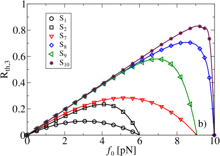
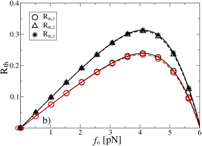
With the increase of to and further to thermodynamic efficiency indeed essentially increases. For the smaller cargo, it reaches a typical experimental value of 50% and even higher already for at pN with the stalling force pN, see in Fig. 8, b. The stalling force is a bit larger than for real kinesins. However, maximal thermodynamical efficiency of about 58% is also larger, as should be for a stronger motor. Nevertheless, this simple model yields indeed realistic efficiencies and stalling forces at the same time. Moreover, our model motor can operate even in the regime of strongly anomalous transport with at the thermodynamic efficiency as large as 70%, for , at pN with stalling force pN, see in Fig. 8, b. This is a real surprise! For smaller cargo the maximal efficiency is even larger, about 83% at , although this transport regime is close to normal. Anomalous subdiffusive transport regime with such a huge efficiency, over 70%, was difficult to expect a priory.
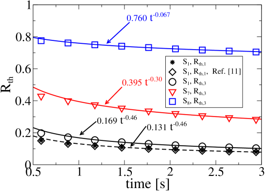
The explanation of this paradoxical behavior reveals a profoundly new feature. Namely, the enzymatic cycling and the potential flashes occur in this case anomalously slow in time with the power law exponent . To understand this we plotted the time-dependence of the thermodynamic efficiencies versus time in Fig. 9 for the sets (here and in Ref. [11]), , and , at taken the values , pN, and , correspondingly (near to the maximum of efficiency vs. ). For , both , and , with confirming that . However, for and , with . Assuming that , one obtains , from which . Hence, from the data in Fig. 9 we deduce that () for and () for . The occurrence of this thermodynamically highly efficient anomalous transport regime, where both the mean transport distance and the mean number of motor turnovers grow sublinearly in time, but with different exponents, presents a profound result of this work, beyond recent treatment in Refs. [10, 11].
4 Summary and Conclusions
In this paper, we further generalized our model of anomalous transport in viscoelastic cytosol of living cells realized by molecular motors like various kinesins. In this model, normally (in the absence of cargo) operating motor is pulling subdiffusive (if not coupled to motor) cargo on an elastic linker, or tether. Subdiffusion is described within non-Markovian GLE approach and its Markovian multi-dimensional embedding realization within a generalized Maxwell-Langevin model of viscoelasticity. The generalization consisted in two aspects. First, we took the mechano-chemical coupling between the motor cyclic turnovers and its translational motion into account within a variant of the model of hand-over-hand motion of kinesin which was introduced in Refs. [40, 43, 42]. It is featured by spatially-dependent rates of conformational transitions. This spatial dependence reflects biochemical cycle kinetics of the molecular motor moving in a periodic binding potential. Our particular model choice was done in accordance with a biophysically plausible requirement that ATP binding to the motor and its hydrolysis can be realized with the same rate anywhere on microtubule. This model choice allowed comparison with the ratchet model in Ref. [11], based on the same requirement, by matching with the doubled enzyme turnover rate in [11], using other parameters the same and for . Second, we considered anharmonic linker with a maximally possible extension length within the FENE model. This model choice allowed a direct comparison with the purely elastic linker model in [11] for the motor-cargo distances less than about one fifth (with 4% accuracy) of the maximal extension length. As a major result of this study, we confirmed within the present more realistic setting, for realistic model parameters, that all the major effects revealed in Refs. [10, 11] not only survives, but also quantitatively are very similar to the results in [11]. This allows to explain how the same motors operating in the same cells can realize both normal and anomalous transport of various cargos depending on the cargo size, strength of the motor (maximal or stall loading force which depends on the amplitude of binding potential), motor operating frequency (which depends on the ATP binding and hydrolysis rate), and the loading force opposing the motion.
However, an important discrepancy between two discussed models emerges on the level of thermodynamic efficiency. Within the present model, the input energy fueling the motor operation is calculated as the energy required to accomplish biochemical cycles of the motor in the working direction by hydrolysing ATP molecules [39, 43, 42], in accordance with the main principles of the free-energy transduction in isothermal engines [55], rather than energy invested into the potential flashes unidirectionally [57]. The former is less than the latter because of the energy recuperation (due to bidirectional coupling). This makes thermodynamic efficiency of molecular motor essentially larger than one obtains in simple ratchet models with unidirectional coupling and constant flashing rates. We showed that our model can consistently explain near to normal transport with thermodynamic efficiency of 50% in viscoelastic environment of biological cells, for realistic parameters. As a major surprise, we showed that a strongly anomalous subdiffusive transport is also possible with thermodynamic efficiencies as high as 70%. Here we revealed a very important new feature. Namely, the biochemical enzyme turnovers can become anomalously slow, , , due to mechanical coupling, not being characterized by a turnover rate anymore. To the best of our knowledge, this is the first time when anomalous enzyme kinetics of this kind, i.e. no mean turnover rate exists, is obtain within a physical approach based on fundamental principles of statistical mechanics [32, 33]. To reveal such a regime provide a real challenge for experimental biophysicists.
It is important to mention that the difference in thermodynamic efficiencies does not affect the major results in Refs. [10, 11] because normally such motors as kinesins are operating at zero thermodynamic efficiency just relocating cargos from one place in the cell to another one, not increasing their potential energy.
Furthermore, we showed that the linker anharmonicity practically does not introduce any significant difference in the case of strong linkers with elastic constant typically used in biophysical literature [65]. However, a recent experiment [21] suggested that the elastic constant can be an order of magnitude lower in viscoelastic environment of living cells as compare with one in water. In Ref. [11], we showed within the model of harmonic linker that the transport of large cargos is hardy possible on such a weak linker when the motor operates at a high turnover frequency of about 100 Hz. The linker should then become broken. However, in the present work we demonstrate that a weak linker can yet sustain such a transport due to strong anharmonic effects. Moreover, we reaffirmed the emergence of a paradoxical regime of cargo’s supertransport with on a weak linker for the motor stepping normally with at its small operating frequencies.
To conclude, we hope that the further confirmation of the major results of [10, 11] in a more realistic setup of this work, as well as new results of this work, will inspire the followup experimental work, which will provide a further feedback to theoretical description of both anomalous and normal transport processes in the viscoelastic crowded environment provided by the cytosol of living cells.
References
References
- [1] Pollard T D, Earnshow W C, Lippincott-Schwartz J 2007 Cell Biology 2nd ed. (Saunders Elsevier, Philadelphia).
- [2] McGuffee S R, Elcock A H 2010 Diffusion, crowding & protein stability in a dynamic molecular model of the bacterial cytoplasm PLoS Comput Biol 6 e1000694.
- [3] Luby-Phelps K 2013 The physical chemistry of cytoplasm and its influence on cell function: an update Mol. Biol. Cell 24 2593.
- [4] Caspi A, Granek R and Elbaum M 2002 Diffusion and directed motion in cellular transport Phys. Rev. E 66 011916.
- [5] Goychuk I 2010 Subdiffusive Brownian ratchets rocked by a periodic force Chem. Phys. 375 450.
- [6] Robert D, Nguyen Th-H, Gallet F and Wilhelm C 2010 In vivo determination of fluctuating forces during endosome trafficking using a combination of active and passive microrheology PLoS ONE 4 e10046.
- [7] Bruno L, Levi V, Brunstein M and Desposito M A 2009 Transition to superdiffusive behavior in intracellular actin-based transport mediated by molecular motors Phys. Rev. E 80 011912.
- [8] Goychuk I and Kharchenko V 2012 Fractional Brownian motors and Stochastic Resonance Phys Rev E 85 051131.
- [9] Kharchenko V and Goychuk I 2012 Flashing subdiffusive ratchets in viscoelastic media New J Phys 14 043042.
- [10] Goychuk I, Kharchenko V and Metzler R 2014 How molecular motors work in the crowded environment of living cells: coexistence and efficiency of normal and anomalous transport PLOS ONE 9 e91700.
- [11] Goychuk I, Kharchenko V and Metzler R 2014 Molecular motors pulling cargos in the viscoelastic cytosol: how power strokes beat subdiffusion Phys. Chem. Chem. Phys. 16 16524.
- [12] Bouzat S 2014 Influence of molecular motors on the motion of particles in viscoelastic media Phys. Rev. E 89 062707.
- [13] Guigas G, Kalla C and Weiss M 2007 Probing the nanoscale viscoelasticity of intracellular fluids in living cells Biophys. J. 93 316.
- [14] Saxton M J and Jacobson K 1997 Single-particle tracking: applications to membrane dynamics Annu. Rev. Biophys. Biomol. Struct. 26 373.
- [15] Qian H 2000 Single-particle tracking: Brownian dynamics of viscoelastic materials Biophys. J. 79 137.
- [16] Yamada S, Wirtz D and Kuo S C 2000 Mechanics of living cells measured by laser tracking microrheology Biophys. J. 78 1736.
- [17] Seisenberger G, Ried M U, Endre Th, Büning H, Hallek M, et al. 2001 Real-time single-molecule imaging of the infection pathway of an adeno-associated virus Science 29 1929.
- [18] Tolić-Nørrelykke I M, Munteanu E-L, Thon G, Oddershede L and Berg-Sørensen K 2004 Anomalous diffusion in living yeast cells Phys. Rev. Lett. 93 078102.
- [19] Golding I and Cox E C 2006 Physical nature of bacterial cytoplasm Phys. Rev. Lett. 96 098102.
- [20] Szymanski J and Weiss M 2009 Elucidating the origin of anomalous diffusion in crowded fluids Phys. Rev. Lett. 103 038102.
- [21] Bruno L, Salierno M, Wetzler D E, Desposito M A, Levi V 2011 Mechanical properties of organelles driven by microtubuli-dependent molecular motors in living cells PLoS ONE 6 e18332.
- [22] Jeon J H, Tejedor V, Burov S, Barkai E, Selhuber-Unkel C, Berg-Sørensen K, Oddershede L and Metzler R 2011 In vivo anomalous diffusion and weak ergodicity breaking of lipid granules Phys. Rev. Lett. 106 048103.
- [23] Jeon J H, Leijnse M , Oddershede L B and Metzler R 2013 Anomalous diffusion and power-law relaxation of the time averaged mean squared displacement in worm-like micellar solutions New J. Phys. 15 045011.
- [24] E. Barkai, Y. Garini and R. Metzler 2012 Strange kinetics of single molecules in living cells Phys. Today 65(8) 29.
- [25] Tabei S M A, Burov S, Kim H Y, Kuznetsov A, Huynh T, Jureller J, Philipson L H, Dinner A R and Scherer N F 2013 Intracellular transport of insulin granules is a subordinated random walk Proc. Natl. Acad. Sci. USA 110 4911.
- [26] Höfling F and Franosch T 2013 Anomalous transport in the crowded world of biological cells Rep. Progr. Phys. 76 046602.
- [27] Taylor M A, Janousek J, Daria V, Knittel J, Hage B, Bachor H-A and Bowen W P 2013 Biological measurement beyond the quantum limit Nature Photonics 7 229.
- [28] Weber S C, Spakowitz A J, Theriot J A 2010 Bacterial chromosomal loci move subdiffusively through a viscoelastic cytoplasm Phys. Rev. Lett. 104 238102.
- [29] Weiss M 2013 Single-particle tracking data reveal anticorrelated fractional Brownian motion in crowded fluids Phys. Rev. E 88 010101 (R).
- [30] Harrison A W, Kenwright D A, Waigh T A, Woodman P G and Allan V J 2013 Modes of correlated angular motion in live cells across three distinct time scales Phys. Biol. 10 036002.
- [31] Hirokawa N and Takemura R 2005 Molecular motors and mechanisms of directional transport in neurons Nature Reviews 6 201.
- [32] Kubo R 1966 The fluctuation-dissipation theorem Rep Prog Phys 29 255.
- [33] Zwanzig R 2001 Nonequilibrium Statistical Mechanics (Oxford University Press, Oxford).
- [34] Mason TG, Weitz DA 1995 Optical measurements of frequency-dependent linear viscoelastic moduli of complex fluids Phys Rev Lett 74 1250.
- [35] Waigh TA 2005 Microrheology of complex fluids Rep Prog Phys 68 685.
- [36] Goychuk I 2009 Viscoelastic subdiffusion: from anomalous to normal Phys. Rev. E 80 046125.
- [37] Goychuk I 2012 Viscoelastic subdiffusion: Generalized Langevin Equation approach Adv. Chem. Phys. 150 187.
- [38] Chauwin J-F, Ajdari A and Prost J 1994 Force-free motion in asymmetric structures: a mechanism without diffusive steps Europhys. Lett. 27 421.
- [39] Jülicher F, Ajdari A and Prost J 1997 Modeling molecular motors Rev. Mod. Phys. 69 1269.
- [40] Astumian R D and Bier M 1996 Mechanochemical coupling of the motion of molecular motors to ATP hydrolysis Biophys. J. 70 637.
- [41] Astumian R D 1997 Thermodynamics and kinetics of a Brownian motor Science 276 917.
- [42] Parmeggiani A, Jülicher F, Ajdari A and Prost J 1999 Energy transduction of isothermal ratchets: Generic aspects and specific examples close to and far from equilibrium Phys. Rev. E 60 2127.
- [43] Jülicher F, Force and motion generation of molecular motors: a generic description, in: Müller S C, Parisi J and Zimmermann W (eds.) 1999 Transport and Structure: Their Competitive Roles in Biophysics and Chemistry (Springer, Berlin) Lect. Not. Phys. 532 46.
- [44] Nelson P 2004 Biological Physics: Energy, Information, Life (Freeman and Co., New York).
- [45] Reimann P 2002 Brownian motors: noisy transport far from equilibrium Phys. Rep. 361 57.
- [46] Makhnovskii Yu A, Rozenbaum V M, Yang D-Y, Lin S H and Tsong T Y 2004 Flashing ratchet model with high efficiency Phys. Rev. E 69 021102.
- [47] Rozenbaum V M, Yang D-Y, Lin S H and Tsong T Y 2004 Catalytic Wheel as a Brownian motor J. Phys. Chem. B 108 15880.
- [48] Perez-Carrasco R and Sancho J M 2010 Theoretical analysis of the -ATPase experimental data Biophys. J. 98 2591.
- [49] Fisher M E and Kolomeisky A B 2001 Simple mechanochemistry describes the dynamics of kinesin molecules Proc Natl Acad Sci USA 98 7748.
- [50] van Kampen NG 1992 Stochastic Processes in Physics and Chemistry, 2nd ed. (North-Holland, Amsterdam).
- [51] Baker N A, Sept D, Joseph S, Holst M J and McCammon J A 2001 Electrostatics of nanosystems: Application to microtubules and the ribosome Proc. Nat. Acad. Sci. USA 98 10037.
- [52] Herrchen M and Öttinger H C 1997 A detailed comparison of various FENE dumbbell models J. Non-Newtonian Fluid Mech. 68 17.
- [53] Kharchenko V and Goychuk I 2013 Subdiffusive rocking ratchets in viscoelastic media: Transport optimization and thermodynamic efficiency in overdamped regime Phys. Rev. E 87 052119.
- [54] Wyman J 1975 The turning wheel: a study in steady states Proc. Nat. Acad. Sci. USA 72 3983.
- [55] Hill T L 1989 Free Energy Transduction and Biochemical Cycle Kinetics (Springer, New York).
- [56] Qian H 2005 Cycle kinetics, steady state thermodynamics and motors – a paradigm for living matter physics J. Phys.: Condens. Matter 17 S3783.
- [57] Sekimoto K 1997 Kinetic characterization of heat bath and the energetics of thermal ratchet models J. Phys. Soc. Jpn. 66 1234.
- [58] Goychuk I and Kharchenko V 2013 Rocking subdiffusive ratchets: origin, optimization and efficiency Math. Model. Nat. Phenom. 8 144.
- [59] Derenyi I, Bier M and Astumian R D 1999 Generalized efficiency and its application to microscopic engines Phys. Rev. Lett. 83 903.
- [60] Suzuki D and Munakata T 2003 Rectification efficiency of a Brownian motor Phys. Rev. E 68 021906.
- [61] Wang H and Oster G 2002 The Stokes efficiency for molecular motors and its applications Europhys. Lett. 57 134.
- [62] Odijk T 2000 Depletion theory of protein transport in semi-dilute polymer solutions Biophys. J. 79 2314.
- [63] Masaro L and Zhu X X 1999 Physical models of diffusion for polymer solutions, gels and solids Prog. Polym. Sci. 24 731.
- [64] Holyst R et al. 2009 Scaling form of viscosity at all length-scales in poly(ethylene glycol) solutions studied by fluorescence correlation spectroscopy and capillary electrophoresis Phys. Chem. Chem. Phys. 11 9025.
- [65] Kojima H, Muto E, Higuchi H and Yanagida T 1996 Mechanics of single kinesin molecules measured by optical trapping nanometry Biophys. J. 73 2012.
- [66] Goychuk I 2012 Is subdiffusional transport slower than normal? Fluct. Noise Lett. 11 1240009.
- [67] Goychuk I 2012 Fractional time random walk subdiffusion and anomalous transport with finite mean residence times: faster, not slower Phys. Rev. E. 86 021113.
- [68] Goychuk I and Kharchenko V O 2014 Anomalous features of diffusion in corrugated potentials with spatial correlations: faster than normal, and other surprises Phys. Rev. Lett. 113 100601.