Lagrangian study of temporal changes of a surface flow through the Kamchatka Strait

Abstract

Using Lagrangian methods we analyze a 20-year-long estimate of water flux through the Kamchatka Strait in the northern North Pacific based on AVISO velocity field. It sheds new light on the flux pattern and its variability on annual and monthly time scales. Strong seasonality in surface outflow through the strait could be explained by temporal changes in the wind stress over the northern and western Bering Sea slopes. Interannual changes in a surface outflow through the Kamchatka Strait correlate significantly with the Near Strait inflow and Bering Strait outflow. Enhanced westward surface flow of the Alaskan Stream across the $174^{\circ}\,\text{E}$ section in the northern North Pacific is accompanied by an increased inflow into the Bering Sea through the Near Strait. In summer, the surface flow pattern in the Kamchatka Strait is determined by passage of anticyclonic and cyclonic mesoscale eddies. The wind stress over the Bering basin in winter – spring is responsible for eddy generation in the region.

1 Introduction

The water circulation in the Bering Sea is tightly connected with a general circulation in the northern North Pacific. It is formed by the cyclonic gyre with two main currents, the Kamchatka Current along the western boundary and the Bering Slope Current in the eastern part of the sea. The most part of Pacific water enters the Bering Sea through the Amukta Pass (Stabeno et al., 2005; Ladd and Stabeno, 2009) and Near Strait (sill depth is about 2000 m) (Fig. 1). The Alaskan Stream, transporting relatively warm subsurface waters, is the main source of waters in the upper 1000 m layer in the Bering Sea. The water outflow from the Bering Sea into the Pacific Ocean occurs mainly through the Kamchatka Strait. The Kamchatka Strait (KS) with its width of 190 km and maximum depth of 4420 m, located between the Kamchatka Peninsula and the Bering Island, occupies 46% of the total area of the straits connecting the Bering Sea and the Pacific Ocean. The water transport through the KS and straits of the Aleutian Island chain is of great importance for the volume, heat and nutrient fluxes between the Bering Sea and the North Pacific (Stabeno et al., 1999). According to various estimates (Overland et al., 1994; Reed, 1995; Cokelet et al., 1996; Panteleev et al., 2006), the volume transport makes up from 5 to 25 Sv ($\text{1~{}Sv}=10^{6}$ m³/s). Speeds of geostrophic flows in the strait, 25–40 cm s^-1, have the maximum in the upper layer (Cokelet et al., 1996). Bering Strait (55 m deep and 85 km wide) provides a connection between the Bering Sea and the Chukchi Sea in the Arctic Ocean. The northward flow through the Bering Strait (${\sim}1$ Sv) is insignificant to the water budget of the deep Bering Sea but it helps balance the freshwater budgets of the Pacific and Atlantic oceans.

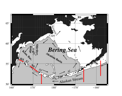
Figure 1: Schematic representation of the currents in the study area. Kom. Bas. — Komandorsky Basin, BS — Bering Strait, KS — Kamchatka Strait, NS — Near Strait, AI — Aleutian Islands, KI — Komandorsky Islands, NI — Near Islands. Thick straight lines show the sections where surface flow anomalies were estimated. Depths more than 1000 m are shaded by grey.

Mesoscale variability is an important factor in the Bering Sea dynamics. The eddy activity in the vicinity of Near Strait has a strong impact on the flow through the strait (Reed and Stabeno, 1993). Generation of anticyclonic and cyclonic submesoscale eddies in Near Strait leads to the flow reversals in central and eastern parts of the strait and westward (or eastward) shift in the velocity core (Prants et al., 2013a). The meanders and eddies are consistent features in the Bering Slope Current and the Kamchatka Current regions (Verkhunov and Tkachenko, 1992; Mizobata et al., 2002). The distributions of the sea surface height anomaly (SSHA) in the KS area and satellite infrared images indicate strong anticyclonic and cyclonic eddy activity in the strait. Although the flux pattern in the KS has been known for decades, volume transport variability and its causes remain highly uncertain because of the lack of direct observations. In this study we analyze a 20-year-long estimate of the water flux through the KS based on AVISO surface velocity fields.

To estimate surface flow in the region we apply in this paper the Lagrangian approach that is based on computing trajectories of passive particles advected by an AVISO velocity field. The domain under study is seeded by a large number of synthetic particles whose trajectories are computed forward or backward in time for a given period of time. When integrating advection equations (1) forward in time one gets an information about fate of water masses and when integrating them backward in time we can determine their origin and history. A graphic view of transport and mixing in a studied area is provided by so-called Lagrangian maps which are plots of one of the Lagrangian indicators versus particle’s initial positions (Uleysky et al., 2007; Prants et al., 2011b, a; Prants, 2013; Prants et al., 2013b). That approach has been successfully applied to study transport and mixing in different basins, from marine bays (Prants et al., 2013b) and seas (Prants et al., 2011a, 2013a) to the ocean scale (Prants et al., 2011b; Prants, 2013).

The Lagrangian approach sheds new insight on the flow patterns in the KS and the variability on annual to monthly time scales. Computed backward-in-time latitudinal Lagrangian maps show mesoscale and submesoscale eddies in the region and origin and history of water masses crossing the strait for a given period of time. We demonstrate in this paper correlations between the outflow flux through the KS, the inflow through the Near Strait, the Bering Strait transport derived from moored observations (Woodgate et al., 2012) and Alaskan Stream surface flow.

2 Data and methods

Since 1992, the ocean surface topography has been continuously observed from the space by the Topex/Poseidon, European Remote Sensing, Geosat Follow-On, Envisat and Jason satellite missions. These data are available at http://www.aviso.oceanobs.com. We use the gridded SSHA for the period of 1993–2012 for diagnostic computations. For each 7-day period, the SSHAs, obtained by optimal interpolation of all available altimeter missions, were downloaded from the AVISO site. In our study, we use the monthly wind stress dataset from the NCEP reanalysis. The horizontal resolution of the NCEP data is $1.9^{\circ}\times 1.9^{\circ}$.

Geostrophic daily velocities, obtained from the AVISO database on a $1/3^{\circ}\times 1/3^{\circ}$ Mercator grid, are an approximation to the real surface fields in the ocean. To provide accurate numerical results we apply a bicubical spatial interpolation and third order Lagrangian polynomials in time. We compute in this paper transport for periods as long as a few weeks. It is reasonably to suppose that various ageostrophic corrections are averaged out for such a long time. Moreover, our results are based not on individual trajectories but on statistics for thousands of trajectories. Most of them have been found to be chaotic with positive values of the maximal finite-time Lyapunov exponent which is an average rate of dispersion of initially closed particles (see, for example, Prants et al., 2011a). Typical chaotic systems are highly robust against a high-frequency noise mimicking small-scale diffusion (see, e. g., Makarov et al., 2006). Individual trajectories are sensitive to small noisy variations in the velocity field but different statistical characteristics and structures like mesoscale manifolds and fronts are not (Hernández-Carrasco et al., 2011; Keating et al., 2011). Thus, an additional small noise in the advection equations is not expected to change our results based on statistics for a large number of particles.

Lagrangian trajectories have been computed by integrating the advection equations with a fourth-order Runge-Kutta scheme

$$\dot{x}=u(x,y,t),\qquad\dot{y}=v(x,y,t),$$ (1)

where time $t$ is in days. Coordinates $x$ and $y$ of a passive particle are related with its latitude $\phi$ and longitude $\lambda$ in degrees as follows:

$$\begin{gathered}\lambda=\frac{x}{60},\quad\phi=\frac{180}{\pi}\arcsin{\tanh{\left(\frac{\pi}{180}\left(\frac{y}{60}+y_{0}\right)\right)}},\\ y_{0}=\frac{180}{\pi}\operatorname{artanh}{\sin{\left(\frac{\pi}{180}\phi_{0}\right)}},\quad\phi_{0}=-82.\end{gathered}$$ (2)

We use the transformation (2) because the AVISO grid is homogeneous in $x\text{--}y$ coordinates. The velocities $u$ and $v$ in Eq. (1) are expressed through the latitudinal $U_{\phi}$ and longitudinal $U_{\lambda}$ components of the linear velocity $U$ in cm s^-1 as follows:

$$u =\frac{10800}{\pi R_{E}\cos\phi}\frac{86400}{100000}U_{\lambda}\approx\frac{0.466}{\cos\phi}U_{\lambda},$$ (3)

$$v =\frac{10800}{\pi R_{E}\cos\phi}\frac{86400}{100000}U_{\phi}\approx\frac{0.466}{\cos\phi}U_{\phi},$$

where $R_{E}=6370$ km is the Earth radius.

The surface fluxes through the KS and the Near Strait have been computed as follows. The lines, crossing the straits from $[163.4^{\circ}\,\text{E}:56.0^{\circ}\,\text{N}]$ to $[165.5^{\circ}\,\text{E}:55.5^{\circ}\,\text{N}]$ and from $[168.5^{\circ}\,\text{E}:54.5^{\circ}\,\text{N}]$ to $[172.3^{\circ}\,\text{E}:53.0^{\circ}\,\text{N}]$, are divided in 20 segments. The flux across each segment was obtained by integrating velocity normal to it at a given point.

3 Results

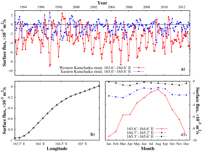
Figure 2: a) Temporal changes in the Kamchatka Strait fluxes, b) flux averaged for 1993–2012 yrs vs longitude, where middles of the intervals are denoted by points, c) monthly averaged flux through different parts of the Kamchatka Strait.

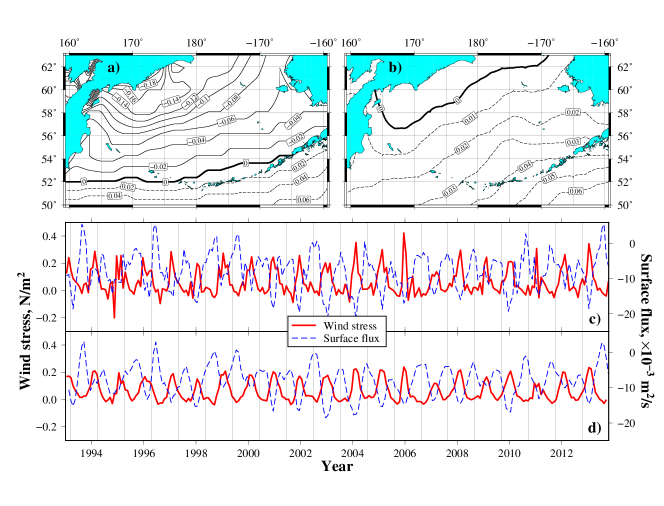
Figure 3: Spatial patterns of zonal wind stress (N m^-2) in the northern North Pacific and Bering Sea in a) November – March and b) July – September c) and d) Time series of the surface flux through the Kamchatka Strait and the wind stress over the Bering Sea ($\tau_{x}^{58^{\circ}\,\text{N},\,165^{\circ}\,\text{E}\text{--}170^{\circ}\,\text{W}}+0.2\tau_{y}^{56\text{--}58^{\circ}\,\text{N},\,165^{\circ}\,\text{E}}$). Low-pass (three-months running mean) filtered series are shown in d).

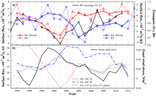
Figure 4: a) The interannual changes of the flux through the Kamchatka and Near Straits and the volume transport through the Bering Sea (http://psc.apl.washington.edu/HLD/Bstrait/Data b) the interannual changes of the surface flux (westward is positive) of the Alaskan Stream (AS) and the zonal wind stress over the northern North Pacific ($52^{\circ}\,\text{N}$, $165^{\circ}\,\text{E}$ – $170^{\circ}\,\text{W}$) averaged for November – March

.

Figures 2a–c show monthly time series of surface fluxes through the western and eastern parts of the KS, the water flux averaged for 1993–2012 years versus longitude and the monthly averaged flux through the different parts of the KS. The computed net flow through the KS is directed from the Bering Sea to the North Pacific. The northward (southward) flow is positive (negative). The surface fluxes of the Alaskan Stream were computed as flows across $174^{\circ}\,\text{E}$ (from $50.0^{\circ}\,\text{N}$ to $52.5^{\circ}\,\text{N}$), $166^{\circ}\,\text{W}$ (from $51.5^{\circ}\,\text{N}$ to $53.5^{\circ}\,\text{N}$) and $158^{\circ}\,\text{W}$ (from $53.0^{\circ}\,\text{N}$ to $55.0^{\circ}\,\text{N}$) lines (Fig. 1). The surface southward flow is enhanced in the western part of the strait, but the flow in its eastern side is relatively weak (Fig. 2b). The flux time series through the western and eastern KS are negatively correlated at the 95% significance level (Fig. 2a). The correlation coefficient is $-0.52$ for the monthly mean values. The negative correlation means that when the southward flow via the western KS is strong, the flow via the eastern KS tends to be northward. A remarkable feature of the surface flux through the KS is relatively high amplitude of its seasonal variations (Fig. 2c). The southward flux through the western part of the KS is strong between November and April and relatively weak in June – September.

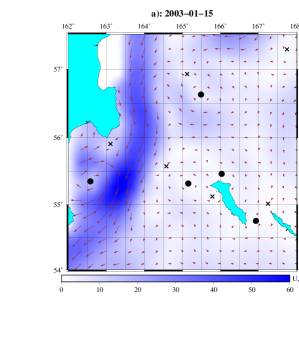
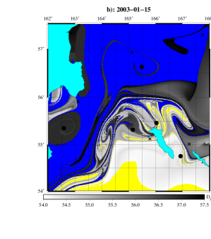
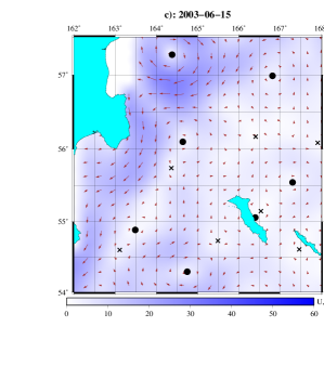
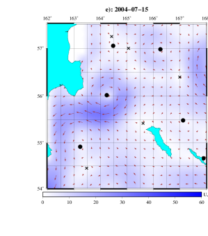
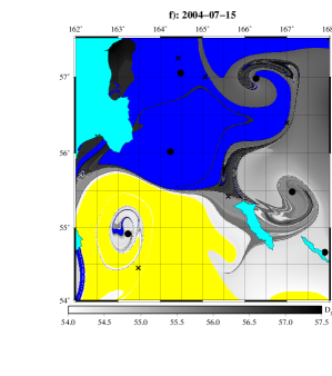
Figure 5: Altimetric velocity fields (a, c and e) and the corresponding latitudinal Lagrangian maps (b, d and f) in the Kamchatka Strait area in winter and summer. Nuances of color on velocity maps measure the modulus of the linear velocity $U$ in cm s^-1. Hyperbolic and elliptic stagnation points are marked by crosses and circles, respectively. The latitudinal maps are computed backward-in-time starting from the date shown to the date which is 180 days before. Dark grey and black colors in geographic degrees code the particles originated from the latitudes north of the strait, ${>}58^{\circ}\,\text{N}$, whereas the light grey and white ones code the particles coming from the latitudes south of the strait, ${<}54^{\circ}\,\text{N}$. (In the web version of this article an additional information is coded by “yellow”and “blue” colors which mark waters that originated outside the domain and advected from the south and north, respectively).

The effect of local wind on the annual variation of the surface flux through the KS may be important due to strong seasonality of the wind forcing (Figs. 3a,b). There is a tendency to have negative (westward and southward) wind stresses over the central and western Bering Sea in winter (Fig. 3a). This wind pattern is favorable for a pile up of the Ekman transport to set up the alongshore jet (Csanady, 1978, 1998) and a sea level rise along the northern and western boundaries of the Bering Sea basin (the Aleutian Basin and the Komandorsky Basin). In summer, the zero wind stress contour extends from the west-southwest to the east-northeast across the central Bering Sea with negative values to its north and positive values to its south (Fig. 3b). Seasonal Ekman forcing is one of the possible causes for a winter maximum of the surface flux through the KS. To assess the effect of the Ekman forcing, we plot in Figs. 3c and 3d the monthly time series of the surface flux through the KS and the wind stress averaged along the northern (from $165^{\circ}\,\text{E}$ to $170^{\circ}\,\text{E}$ along $58^{\circ}\,\text{N}$) and western (from $56^{\circ}\,\text{N}$ to $58^{\circ}\,\text{N}$ along $165^{\circ}\,\text{E}$) Bering Sea slope segments ($\tau_{x}^{58^{\circ}\,\text{N},\,165^{\circ}\,\text{E}\text{--}170^{\circ}\,\text{W}}+0.2\tau_{y}^{56\text{--}58^{\circ}\,\text{N},\,165^{\circ}\,\text{E}}$, where $0.2$ is the ratio between the length of the western and northern Bering Sea slope segments). The similar approach was used for an examination of the SSHA along the Alaska/Canada coast from the TOPEX/Poseidon data (Qiu, 2002) and the tide gauge sea level data along the northern and western coasts of the Okhotsk Sea (Nakanowatari and Ohshima, 2013). Our results show a good correspondence ($r=-0.59$, unfiltered series in Fig. 3c) and $-0.69$ (low-pass filtered series Fig. 3d) between the monthly time-series signals of the surface flux through the KS and the wind stress $\tau_{L}$. The monthly time series of the volume transport along the continental slope of the KS (computed as $\tau_{L}L/(f\rho)$, where $L$ is the total length of the northern and western Bering basin segments, $\rho$ is the density of water and $f$ is the Coriolis parameter) exhibit a strong seasonal cycle with peak southward (negative) transport of 6–8 Sv in winter and near-zero or positive (${\sim}2$ Sv) transport in summer.

The bulk of inflow into the Bering Sea occurs through the Near Strait at the western end of the Aleutian Islands ($168^{\circ}\,\text{E}$ – $172^{\circ}\,\text{E}$). Figure 4a demonstrates year-to-year changes of the water flux through the KS (averaged for January – September) and the Near Strait, and the volume transport through the Bering Strait derived from 20-year moored observations (Woodgate et al., 2012). Enhanced water inflow from the Pacific Ocean to the Bering Sea through the Near Strait accompanies increased outflow through the KS ($r=-0.67$, 1993–2012, low-pass filtered series) and the Bering Strait ($r=0.78$, 1993–2011). On the interannual time scale, the positive correlation ($r=0.48$) is diagnosed between the flow into the Bering Sea through the Near Strait and the Alaskan Stream surface flow through the $174^{\circ}\,\text{E}$ section (Fig. 4b). Stronger Alaskan Stream in the Near Islands area appears to increase NS inflow. But there is a negative correlation between the NS inflow and the Alaskan Stream surface flow through the $158^{\circ}\,\text{W}$ section ($r=-0.67$).

In winter, the surface flow pattern in the KS is determined by a strong stream directed from the Bering Sea to the Pacific Ocean via the western part of the strait (see the altimetric velocity field on 15 January, 2003 in Fig. 5a). In order to get a more detailed information about transport through KS, we compute latitudinal Lagrangian maps. The domain under study is seeded with a large number of synthetic particles which are advected backward in time by the AVISO velocity field starting from a given day to a day in the past. The latitude from which each particle came to its final position during that period of time is coded by color. Figure 5b shows meridional displacements of markers during the second half of 2002 with dark grey and black colors in geographic degrees coding the particles originated from the latitudes north of the strait (${>}58^{\circ}\,\text{N}$), whereas the light grey and white colors code the particles coming from the latitudes south of the strait (${<}54^{\circ}\,\text{N}$). Hyperbolic and elliptic stagnation points, where the velocity is found to be zero, are marked in this figure by crosses and circles, respectively. Motion around “trivial” elliptic points is stable, and they are situated, as a rule, in the centers of eddies. Unstable hyperbolic or saddle points organize fluid motion in their neighbourhood in a specific way: particles approach that point along two stable directions and quit it along the other two unstable directions.

In summer, according to cruise data (Verkhunov and Tkachenko, 1992), satellite altimetry data and infrared satellite images, the flow pattern through the KS is induced mainly by mesoscale eddies in the strait. In June 2003, the cyclonic eddy perturbed the surface flow in KS, enhancing the southward flow in the middle of the strait and causing northward flow on the western side. The net flux through the KS was directed from the Bering Sea into the North Pacific (Figs. 5c and d). In summer of the next year, a mesoscale anticyclone in KS centered at $[164.25^{\circ}\,\text{E}:56^{\circ}\,\text{N}]$ and a mesoscale cyclone $[163.25^{\circ}\,\text{E}:{\approx}55^{\circ}\,\text{N}]$ to the south blocked flow through the strait (Figs. 5e and f).

The flow, directed from the ocean to the Bering Sea in the eastern part of the KS, is accompanied by a flow, directed from the Bering Sea to the ocean in the western part of the KS ($r=-0.74$), and vice versa (Fig. 6a). The year-to-year changes in the fluxes through the western and eastern parts of the KS in June – September are correlated ($r=0.55$ and $-0.57$) with the 1-year lagged zonal wind stress over the Bering basin, $\tau_{x}^{58^{\circ}\,\text{N},\,165^{\circ}\,\text{E}\text{--}170^{\circ}\,\text{W}}$, in January – April (Fig. 6a). Increased/decreased westward component of the wind stress over the Bering basin in winter leads to generation of negative/positive SSHAs along the Bering slope off the Navarin Cape and in Shirshov Ridge area ($r=0.57\text{--}0.79$) (Fig. 6b). These SSHAs could be observed in KS area with a 1-year lag (Fig. 6c). The correlation coefficient between the SSHA time-series in KS area and the 1-year lagged SSHA along the northern and western Bering slope in spring – fall is $0.84$.

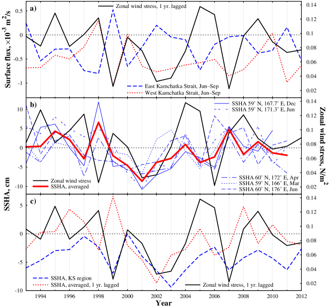
Figure 6: Year-to-year changes of the surface flux through the Kamchatka Strait in June – September (a), sea surface height anomaly (SSHA) in the Bering Sea (b and c) and the zonal wind stress ($56^{\circ}\,\text{N}$ – $58^{\circ}\,\text{N}$, $165^{\circ}\,\text{E}$ – $170^{\circ}\,\text{W}$) over the Bering Sea averaged for January – April (a–c).

4 Discussion

4.1 Spatial and temporal variation of the surface flow

The annual modulation in the Bering Sea gyre intensity may be interpreted as a barotropic response to seasonal wind stress curl forcing. The magnitude of this response is quantifiable by a time-dependent Sverdrup balance (Bond et al., 1994). Our results (Fig. 3c) demonstrate that seasonal wind stress forcing is one of possible reasons for the winter maximum of the surface flux through the KS. Based on results of a numerical model simulation, it has been found that monthly mean volume flux time series through the Near Strait and the KS were significantly correlated with the correlation coefficient $-0.80$ (Clement Kinney and Maslowski, 2012). The correlation essentially means that when inflow into the Bering Sea via the Near Strait is strong, outflow via the KS also tends to be strong and vice versa. Correlations between volume transport through the KS and the passes east of the Near Strait are much lower in magnitude (from $0.15$ to $0.27$) and, therefore, less important than correlation between the KS and the Near Strait (Clement Kinney and Maslowski, 2012). On the interannual scale, we diagnosed the statistically significant correlation ($r=-0.67$, 1993–2012) between inflow into the Bering Sea through the Near Strait and outflow through the KS (Fig. 4a). On the seasonal time scale, we did not observe a statistically significant correlation between Near Strait inflow and outflow via the KS. The main outflow through the KS occurs from November to April (Fig. 2c). But the monthly averaged inflows via the Near Strait in winter are only 20 percent higher than those in summer.

The changes in the Alaskan Stream transport may be one of the main causes of variability in water inflow via the Aleutian Passes and outflow through the KS. Based on results of the ocean circulation model simulation, it has been demonstrated that an increase of the Alaskan Stream transport from 10 to 25 Sv causes warming and sea level rise in the Bering Sea shelf due to increased transport of warmer Pacific waters through the eastern passages of the Aleutian Islands (Ezer and Oey, 2010). An increase of the Alaskan Stream transport from 25 to 40 Sv had an opposite impact on the Bering Sea shelf with a slight cooling (Ezer and Oey, 2010). By using SSHA observed by satellites in 1992–2010 and monthly climatology of temperature and salinity, it has been found by Panteleev et al. (2012) a significant negative correlation ($r=-0.84$) between the low-pass filtered series of the Near Strait inflow and the Alaskan Stream transport across the $158^{\circ}\,\text{W}$ section. The stronger Alaskan Stream appears to reduce the Near Strait inflow and at the same time produces a larger transport through the Aleutian Arc which amplifies the main cyclonic gyre controlled by the continental slope within the Bering Slope Current region (Panteleev et al., 2012).

The surface anomalies of the Near Strait inflow and the Alaskan Stream flow across $158^{\circ}\,\text{W}$ computed by us are in a good agreement with the transport anomalies calculated by Panteleev et al. (2012). On the interannual scale, we obtain a negative correlation between the Alaskan Stream flow across $158^{\circ}\,\text{W}$ and the Near Strait inflow ($r=-0.67$). However, our results demonstrate (Figs. 4a and b) that there is a positive correlation between the Alaskan Stream flow across $174^{\circ}\,\text{E}$ (the Near Islands area) and the Near Strait inflow ($r=0.48$). It means that the Near Strait inflow is amplified when the Alaskan Stream in the Near Islands area is relatively strong. There is a significant difference between the time-series of the Alaskan Stream flux across $174^{\circ}\,\text{E}$ (the western Aleutian Islands area), $166^{\circ}\,\text{W}$ (the eastern Aleutian Islands area) and $158^{\circ}\,\text{W}$ (the Alaska region) (Fig. 4b). The $158^{\circ}\,\text{W}$ section crosses the northern boundary of the Alaska cyclonic gyre. The difference in the Alaskan Stream fluxes across $174^{\circ}\,\text{E}$, $166^{\circ}\,\text{W}$ and $158^{\circ}\,\text{W}$ sections may be caused by a recirculation of the Alaskan Stream waters in the Alaska gyre. A part of the Alaskan Stream waters inflows into the Bering Sea through the Aleutian Passes located eastward of the Near Strait ($172^{\circ}\,\text{E}$ – $166^{\circ}\,\text{W}$).

Interannual variation in the surface flux of the Alaskan Stream across $174^{\circ}\,\text{E}$ and the surface flux through the Near Strait correlate with changes in along Aleutian Islands wind stress. The correlation coefficients between the zonal wind stress ($52^{\circ}\,\text{N}$, $165^{\circ}\,\text{E}$ – $170^{\circ}\,\text{W}$), averaged for November – March, and annually averaged surface flux of the Alaskan Stream (Fig. 4b) and the surface flux through the Near Strait are $-0.58$ and $-0.74$ (low-pass filtered series). In November – March, the Aleutian Low develops in the North Pacific, strong westward winds appear in the Bering Sea, and eastward winds prevail in the northern North Pacific (Fig. 3a). An increased westward winds (negative values of the zonal wind stress) over the Aleutian Islands in November – March may force a westward surface flow of the Alaskan Stream and enhanced water flux via the Near Strait into the Bering Sea.

4.2 Eddy impact on the flow through the Kamchatka Strait

The flow pattern in the KS during summer (June – September) is determined by strength of cyclonic and anticyclonic eddies in the strait area. Passing of a cyclone through the KS enhances a southward flux on the western side of the strait and a northward flux on its eastern side (Fig. 5d). Anticyclones typically increase northward flux through the western KS and southward flux through the eastern KS. In some summers, there appears a cyclonic companion of the anticyclone in the strait. Such a vortex pair practically blocks water exchange through the KS. The Lagrangian map in Fig. 5e demonstrates that effect in July, 2004. There is a strong negative correlation ($r=-0.74$) between the surface fluxes via the western and eastern parts of the strait averaged for June – September (Fig. 6a).

Observations of eddies in the Bering Sea basin have been made by the authors of papers Verkhunov and Tkachenko (1992); Stabeno and Reed (1994); Cokelet et al. (1996); Mizobata et al. (2002) and others. The model results over the 26-year simulation, 1974–2000 (Maslowski et al., 2008) show frequent and complex eddy activity in the Bering Sea with lifetimes of the order of a few months. Half of the eddies is anticyclonic and the other half is cyclonic. Diameters of those eddies are 120 km and greater and velocities are up to 40 cm s^-1. Instabilities along the Bering Slope and the Kamchatka Current and interactions with canyons and embayments at the landward edge of these currents, as well as inflows through the Aleutian Islands Passes, may be responsible for eddy generation in this region (Kinder et al., 1980; Cokelet et al., 1996).

5 Conclusions

1. The surface southward flux through the Kamchatka Strait demonstrates relatively high amplitude of its seasonal variations. The southward flow through the strait is strong between November and April and relatively weak in June – September. The strong seasonality in surface outflow through the Kamchatka Strait can be explained by temporal changes in the wind stress over the northern and western Bering Sea slopes.

2. The interannual changes in a surface outflow through the Kamchatka Strait statistically significantly correlate with Near Strait inflow and Bering Strait outflow. Enhanced westward surface flux of the Alaskan Stream across the $174^{\circ}\,\text{E}$ section in the northern North Pacific is accompanied by an increased inflow into the Bering Sea through the Near Strait.

3. In summer, the surface flow pattern in the Kamchatka Strait is determined by passing of anticyclonic and cyclonic eddies. Those eddies are formed in the central and western Bering Sea with wind stress over the Bering basin in winter – spring to be responsible for eddy generation in the region.

References

- Bond et al. (1994) Bond, N.A., Overland, J.E., Turet, P., 1994. Spatial and temporal characteristics of the wind forcing of the bering sea. Journal of Climate 7, 1119–1130. doi:10.1175/1520-0442(1994)007<1139:SATCOT>2.0.CO;2.
- Clement Kinney and Maslowski (2012) Clement Kinney, J., Maslowski, W., 2012. On the oceanic communication between the western subarctic gyre and the deep bering sea. Deep Sea Research Part I: Oceanographic Research Papers 66, 11–25. doi:10.1016/j.dsr.2012.04.001.
- Cokelet et al. (1996) Cokelet, E.D., Schall, M.L., Dougherty, D.M., 1996. Adcp-referenced geostrophic circulation in the bering sea basin. Journal of Physical Oceanography 26, 1113–1128. doi:10.1175/1520-0485(1996)026<1113:ARGCIT>2.0.CO;2.
- Csanady (1978) Csanady, G.T., 1978. The arrested topographic wave. Journal of Physical Oceanography 8, 47–62. doi:10.1175/1520-0485(1978)008<0047:TATW>2.0.CO;2.
- Csanady (1998) Csanady, G.T., 1998. The non-wavelike response of a continental shelf to wind. Journal of Marine Research 56, 773–788. doi:10.1357/002224098321667350.
- Ezer and Oey (2010) Ezer, T., Oey, L.Y., 2010. The role of the alaskan stream in modulating the bering sea climate. Journal of Geophysical Research 115. doi:10.1029/2009JC005830.
- Hernández-Carrasco et al. (2011) Hernández-Carrasco, I., López, C., Hernández-García, E., Turiel, A., 2011. How reliable are finite-size Lyapunov exponents for the assessment of ocean dynamics? Ocean Modelling 36, 208–218. doi:10.1016/j.ocemod.2010.12.006.
- Keating et al. (2011) Keating, S.R., Smith, K.S., Kramer, P.R., 2011. Diagnosing Lateral Mixing in the Upper Ocean with Virtual Tracers: Spatial and Temporal Resolution Dependence. J. Phys. Oceanogr. 41, 1512–1534. doi:10.1175/2011JPO4580.1.
- Kinder et al. (1980) Kinder, T.H., Schumacher, J.D., Hansen, D.V., 1980. Observation of a baroclinic eddy: An example of mesoscale variability in the bering sea. Journal of Physical Oceanography 10, 1228–1245. doi:10.1175/1520-0485(1980)010<1228:OOABEA>2.0.CO;2.
- Ladd and Stabeno (2009) Ladd, C., Stabeno, P.J., 2009. Freshwater transport from the pacific to the bering sea through amukta pass. Geophysical Research Letters 36. doi:10.1029/2009GL039095.
- Makarov et al. (2006) Makarov, D., Uleysky, M., Budyansky, M., Prants, S., 2006. Clustering in randomly driven hamiltonian systems. Physical Review E 73. doi:10.1103/PhysRevE.73.066210.
- Maslowski et al. (2008) Maslowski, W., Roman, R., Kinney, J.C., 2008. Effects of mesoscale eddies on the flow of the alaskan stream. Journal of Geophysical Research 113. doi:10.1029/2007JC004341.
- Mizobata et al. (2002) Mizobata, K., Saitoh, S., Shiomoto, A., Miyamura, T., Shiga, N., Imai, K., Toratani, M., Kajiwara, Y., Sasaoka, K., 2002. Bering sea cyclonic and anticyclonic eddies observed during summer 2000 and 2001. Progress in Oceanography 55, 65–75. doi:10.1016/S0079-6611(02)00070-8.
- Nakanowatari and Ohshima (2013) Nakanowatari, T., Ohshima, K.I., 2013. Coherent sea level variability in and around the sea of okhotsk. Progress in Oceanography (submitted) .
- Overland et al. (1994) Overland, J.E., Spillane, M.C., Hurlburt, H.E., Wallcraft, A.J., 1994. A numerical study of the circulation of the bering sea basin and exchange with the north pacific ocean. Journal of Physical Oceanography 24, 736–758. doi:10.1175/1520-0485(1994)024<0736:ANSOTC>2.0.CO;2.
- Panteleev et al. (2012) Panteleev, G., Yaremchuk, M., Luchin, V., Nechaev, D., Kukuchi, T., 2012. Variability of the bering sea circulation in the period 1992–2010. Journal of Oceanography 68, 485–496. doi:10.1007/s10872-012-0113-0.
- Panteleev et al. (2006) Panteleev, G.G., Stabeno, P., Luchin, V.A., Nechaev, D.A., Ikeda, M., 2006. Summer transport estimates of the kamchatka current derived as a variational inverse of hydrophysical and surface drifter data. Geophysical Research Letters 33. doi:10.1029/2005GL024974.
- Prants et al. (2013a) Prants, S., Andreev, A., Budyansky, M., Uleysky, M., 2013a. Impact of mesoscale eddies on surface flow between the pacific ocean and the bering sea across the near strait. Ocean Modelling 72, 143–152. doi:10.1016/j.ocemod.2013.09.003.
- Prants et al. (2011a) Prants, S., Budyansky, M., Ponomarev, V., Uleysky, M., 2011a. Lagrangian study of transport and mixing in a mesoscale eddy street. Ocean Modelling 38, 114–125. doi:10.1016/j.ocemod.2011.02.008.
- Prants (2013) Prants, S.V., 2013. Dynamical systems theory methods to study mixing and transport in the ocean. Physica Scripta 87, 038115. doi:10.1088/0031-8949.
- Prants et al. (2013b) Prants, S.V., Ponomarev, V.I., Budyansky, M.V., Uleysky, M.Y., Fayman, P.A., 2013b. Lagrangian analysis of mixing and transport of water masses in the marine bays. Izvestiya, Atmospheric and Oceanic Physics 49, 82–96. doi:10.1134/S0001433813010088.
- Prants et al. (2011b) Prants, S.V., Uleysky, M.Y., Budyansky, M.V., 2011b. Numerical simulation of propagation of radioactive pollution in the ocean from the Fukushima Dai-ichi nuclear power plant. Doklady Earth Sciences 439, 1179–1182. doi:10.1134/S1028334X11080277.
- Qiu (2002) Qiu, B., 2002. Large-scale variability in the midlatitude subtropical and subpolar north pacific ocean: Observations and causes. Journal of Physical Oceanography 32, 353–375. doi:10.1175/1520-0485(2002)032<0353:LSVITM>2.0.CO;2.
- Reed (1995) Reed, R.K., 1995. On geostrophic reference levels in the bering sea basin. Journal of Oceanography 51, 489–498. doi:10.1007/BF02286394.
- Reed and Stabeno (1993) Reed, R.K., Stabeno, P.J., 1993. The recent return of the Alaskan Stream to Near Strait. Journal of Marine Research 51, 515–527. doi:10.1357/0022240933224025.
- Stabeno et al. (2005) Stabeno, P.J., Kachel, D.G., Kachel, N.B., Sullivan, M.E., 2005. Observations from moorings in the aleutian passes: temperature, salinity and transport. Fisheries Oceanography 14, 39–54. doi:10.1111/j.1365-2419.2005.00362.x.
- Stabeno and Reed (1994) Stabeno, P.J., Reed, R.K., 1994. Circulation in the bering sea basin observed by satellite-tracked drifters: 1986–1993. Journal of Physical Oceanography 24, 848–854. doi:10.1175/1520-0485(1994)024<0848:CITBSB>2.0.CO;2.
- Stabeno et al. (1999) Stabeno, P.J., Schumacher, J.D., Ohtani, K., 1999. The physical oceanography of the Bering Sea, in: Loughlin, T., Ohtani, K. (Eds.), Dynamics of the Bering Sea: A Summary of Physical, Chemical, and Biological Characteristics, and a Synopsis of Research on the Bering Sea. University of Alaska Sea Grant. volume 99 of Alaska Sea Grant College Program report, pp. 1–28.
- Uleysky et al. (2007) Uleysky, M.Y., Budyansky, M.V., Prants, S.V., 2007. Effect of dynamical traps on chaotic transport in a meandering jet flow. Chaos: An Interdisciplinary Journal of Nonlinear Science 17, 043105. doi:10.1063/1.2783258.
- Verkhunov and Tkachenko (1992) Verkhunov, A.V., Tkachenko, Y.Y., 1992. Recent observations of variability in the western bering sea current system. Journal of Geophysical Research 97, 14369. doi:10.1029/92JC01196.
- Woodgate et al. (2012) Woodgate, R.A., Weingartner, T.J., Lindsay, R., 2012. Observed increases in bering strait oceanic fluxes from the pacific to the arctic from 2001 to 2011 and their impacts on the arctic ocean water column. Geophysical Research Letters 39, L24603. doi:10.1029/2012GL054092.