The Massive and Distant Clusters of WISE Survey. III. Sunyaev-Zel’dovich Masses of Galaxy Clusters at
Abstract
We present CARMA 30 GHz Sunyaev-Zel’dovich (SZ) observations of five high-redshift (), infrared-selected galaxy clusters discovered as part of the all-sky Massive and Distant Clusters of WISE Survey (MaDCoWS). The SZ decrements measured toward these clusters demonstrate that the MaDCoWS selection is discovering evolved, massive galaxy clusters with hot intracluster gas. Using the SZ scaling relation calibrated with South Pole Telescope clusters at similar masses and redshifts, we find these MaDCoWS clusters have masses in the range . Three of these are among the most massive clusters found to date at , demonstrating that MaDCoWS is sensitive to the most massive clusters to at least . The added depth of the AllWISE data release will allow all-sky infrared cluster detection to and beyond.
Subject headings:
cosmology: observations — galaxies: clusters: general — galaxies: clusters: intracluster medium — galaxies: high redshift — infrared: galaxies1. Introduction
The last decade, roughly since the launch of the Spitzer Space Telescope, has been a remarkably productive time for the discovery of high-redshift () galaxy clusters. This is due in large part to Spitzer’s superb sensitivity to massive galaxies out to very high redshift, but also to the maturation of Sunyaev-Zel’dovich (SZ) effect surveys and increasingly sophisticated X-ray and radio active galactic nucleus (AGN)-based surveys. These techniques have successfully identified galaxy clusters beyond (e.g., Rosati et al., 2004; Mullis et al., 2005; Stanford et al., 2006; Eisenhardt et al., 2008; Muzzin et al., 2009; Brodwin et al., 2010; Galametz et al., 2010; Brodwin et al., 2013; Zeimann et al., 2013; Reichardt et al., 2013; Hasselfield et al., 2013; Bleem et al., 2015) and even at (e.g., Fassbender et al., 2011b; Santos et al., 2011; Stanford et al., 2012; Zeimann et al., 2012; Muzzin et al., 2013; Bayliss et al., 2014; Willis et al., 2013; Newman et al., 2014).
Despite their successes in discovering high-redshift clusters, deep X-ray (e.g., Fassbender et al., 2011a; Mehrtens et al., 2012) and Spitzer surveys (e.g., Eisenhardt et al., 2008; Papovich et al., 2010; Rettura et al., 2014) are limited to relatively small areas ( deg2), and thus do not probe the volume required to meaningfully sample the high-mass end of the cluster mass function. The South Pole Telescope (SPT, Reichardt et al., 2013; Bleem et al., 2015) and Atacama Cosmology Telescope (ACT, Hasselfield et al., 2013) SZ surveys, though much larger, are still limited to a few thousand square degrees, whereas the all-sky Planck SZ survey (Planck Collaboration et al., 2014) is limited to due to its large beam.
The Massive and Distant Clusters of WISE Survey (MaDCoWS, Gettings et al., 2012; Stanford et al., 2014) is a new IR-selected galaxy cluster survey based on the all-sky catalogs of the Wide-field Infrared Survey Explorer (WISE, Wright et al., 2010). The combination of WISE infrared and Sloan Digital Sky Survey (SDSS) DR8 optical photometry (Aihara et al., 2011) allows us to robustly isolate galaxy clusters at in the northern hemisphere. The first spectroscopically confirmed MaDCoWS cluster, MOO J2342+1301 at , was reported by Gettings et al. (2012). The reader is referred to that paper, along with the upcoming survey paper (Gonzalez et al. in prep), for a more complete description of the survey methodology.
The current 10,000 deg2 survey footprint is four times larger than the SPT-SZ survey (Bleem et al., 2015) and 1000 times larger than the area of the IRAC Distant Cluster Survey (IDCS), in which the most massive galaxy cluster known to date was found (Brodwin et al., 2012; Stanford et al., 2012; Gonzalez et al., 2012). Given the unprecedented volume surveyed at high redshift, the MaDCoWS sample should contain a large number of very massive, distant clusters.
In this paper we present Combined Array for Research in Millimeter-wave Astronomy111http://www.mmarray.org (CARMA) 30 GHz observations of five MaDCoWS clusters spanning a range of infrared richnesses. The spectroscopic confirmations for all but one of these clusters are given in Stanford et al. (2014). In §2 we present the MaDCoWS clusters, including a (red sequence) photometric redshift measurement for MOO J1014+0038, and describe the CARMA SZ observations. In §3 we describe the measurements of total Comptonization, from which we infer masses. We discuss our results in §4. We assume a concordance CDM cosmology with , and km s-1 Mpc-1. Spitzer/IRAC and ground-based optical magnitudes are calibrated to the Vega and AB systems, respectively.
2. Data
2.1. CARMA Observations
CARMA is an interferometer that consists of six 10.4 m, nine 6.1 m, and eight 3.5 m telescopes, providing fields of view of FWHM 3.8′, 6.6′ and 11.4′ at 30 GHz, respectively. All 23 telescopes have 30 and 90 GHz receivers, while the 10.4 m and 6.1 m telescopes have an additional 230 GHz receiver. CARMA is equipped with two correlators: an 8-station correlator with 7.5 GHz of bandwidth per baseline (the “wideband correlator”) and a more flexible correlator that can be configured to correlate 23 stations with 2 GHz bandwidth per baseline at 30 GHz (“spectral line correlator”). To maximize sensitivity, both correlators can be used simultaneously.
Clusters MOO J0012+1602, MOO J0319-0025 and MOO J1014+0038 were observed when the 10.4 m and 6.1 m telescopes were in E configuration, the 3.5 m telescopes were in SL configuration, and the signals were processed by both correlators (“E+SL”). MOO J1155+3901 was observed using the wideband correlator and the eight 3.5 m telescopes in the SH configuration. MOO J1514+1346 was observed twice, first using the eight 3.5 m telescopes in the SL configuration with the wideband correlator and later with all 23 telescopes in the E+SL configuration using only the spectral line correlator. All observations were centered around 31 GHz.
With the exception of MOO J1514+1346, cluster observations in the E+SL configuration used the wideband correlator to process the intermediate frequency (IF) signal from eight of the 6.1 m telescopes. The synthesized beam formed by the 6.1 m 6.1 m baselines is approximately 1′, a resolution well matched to the angular size of the SZ signal from these distant clusters. The wideband correlator provides most of the sensitivity to the cluster signal in these observations. The 23-element observations of MOO J1514+1346 lacked the wideband correlator due to a hardware problem and were primarily useful for confirming a point source that was not well detected by the SL data alone. For the standard E+SL observations, the spectral line correlations sample baselines from 0.35-12.0 k, while the wideband correlations sample baselines from 0.65-4.0 k.
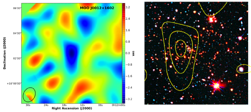
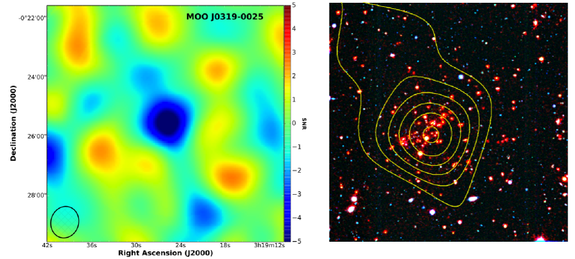
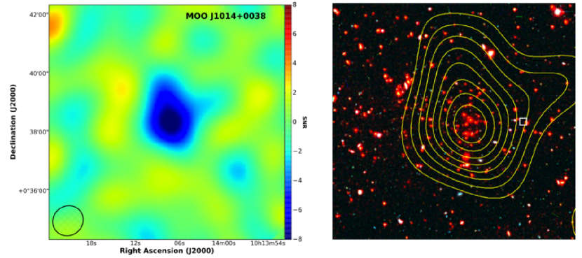
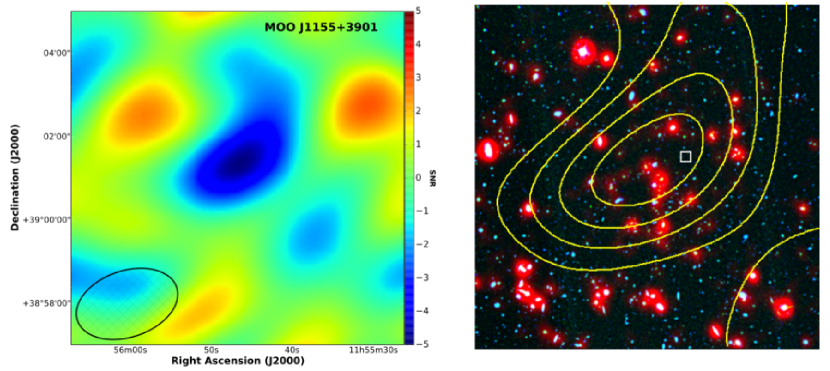
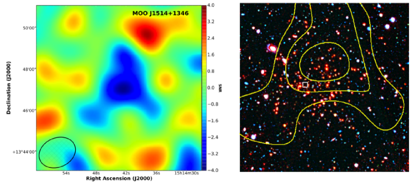
The CARMA observations, summarized in Table 1, used the WISE centroid positions as the pointing and phase centers. The data were reduced with a pipeline using MIRIAD (Sault et al., 1995) similar in function to the one described in Muchovej et al. (2007). After filtering for bad weather and instrumentation problems, the data were gain-calibrated using observations of bright, unresolved quasars interleaved every 15 minutes between the cluster observations. Flux densities are calibrated against observations of Mars using the model presented in Rudy et al. (1987). The pipeline produces a set of flux-calibrated visibilities of the cluster field. The CARMA images in Figure 1 are created by combining naturally-weighted data from both correlators. They are in SNR units and a 2 k cutoff is applied to the data to highlight the cluster-sensitive baselines in the images. Models fit to emissive sources are removed (see §3.1). The residual maps are CLEANed inside a square box 3′ on a side, centered on the position of the map with the largest absolute value in SNR units. CLEAN is allowed to proceed until the largest peak in the map is 1.5 times the map RMS value.
| Cluster ID | R.A. | Decl. | UT Dates | CARMA Array | Exp. Time11Total on-source exposure time, excluding overhead, calibrations and flagged (unused) data. | Map RMS Noise22The map RMS noise is the mean noise within a 3.5′ radius circle centered on the pointing center. |
|---|---|---|---|---|---|---|
| (J2000) | (J2000) | (hr) | (mJy) | |||
| MOO J00121602 | 00:12:13.0 | 16:02:15 | 2013 Sep 24; Oct 1,3,6 | E+SL | 6.0 | 0.11 |
| MOO J03190025 | 03:19:24.4 | 00:25:21 | 2013 Sep 30 | E+SL | 1.0 | 0.26 |
| MOO J10140038 | 10:14:08.4 | 00:38:26 | 2013 Oct 6-7 | E+SL | 2.2 | 0.17 |
| MOO J11553901 | 11:55:45.6 | 39:01:15 | 2012 May 11-12 | SH | 7.2 | 0.33 |
| MOO J15141346 | 15:14:42.7 | 13:46:31 | 2013 Jun 1,3,5-7,9,11 | SL | 8.4 | 0.20 |
| 2013 Aug 15 | E+SL | 0.5 | 0.19 |
| Cluster ID | R.A. | Decl. | Flux |
|---|---|---|---|
| (J2000) | (J2000) | (mJy) | |
| MOO J00121602 | 00:12:14.39 | 16:02:23.6 | |
| MOO J03190025 | - | - | - |
| MOO J10140038 | 10:14:03.84 | 00:38:26.0 | |
| MOO J11553901 | 11:55:44.36 | 39:01:28.6 | |
| MOO J15141346 | 15:14:33.59 | 13:52:47.3 | $\dagger$$\dagger$This is an extended radio source 6′ NW of the phase center. The flux was measured in an elliptical aperture with a 16″ semi-major axis and an axial ratio of 0.72. |
| 15:14:44.57 | 13:46:34.8 |
2.2. Gemini Data
All but one of these clusters (MOO J1014+0038) were observed with the Gemini Multi-Object Spectrograph (GMOS) on Gemini-North. Exposure times of 15 min were obtained in the - and -bands to produce color magnitude diagrams (CMDs) from which red-sequence members could be selected for follow-up spectroscopic observations. These images are combined with IRAC 3.6 m or WISE 3.4 m images to make the color images for four of the five clusters shown in Figure 1.
These images were used to construct several of the masks, for both Gemini/GMOS-N and Keck/DEIMOS, with which we spectroscopically confirmed 20 MaDCoWS clusters to date, including four of the five in the present work. Stanford et al. (2014) provide a full description of the MaDCoWS spectroscopy.
2.3. Magellan Data
Cluster MOO J1014+0038 was observed on UT 2014 January 22 with the Inamori Magellan Areal Camera and Spectrograph (IMACS; Dressler et al., 2006) in the , and bands for 2, 12, and 12 minutes, respectively. These data were reduced with the SPT optical pipeline, as described in Song et al. (2012), and the and images are combined with IRAC 3.6 m to make the color image of this cluster shown in Figure 1.
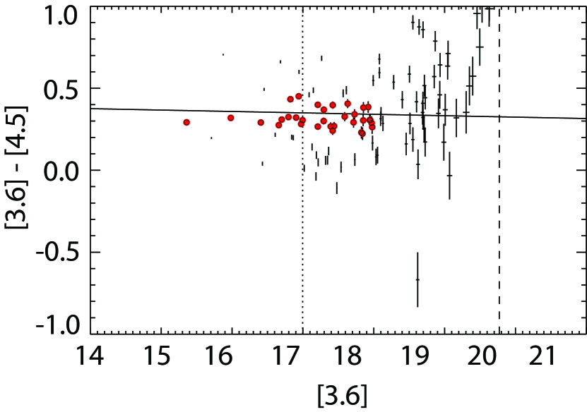
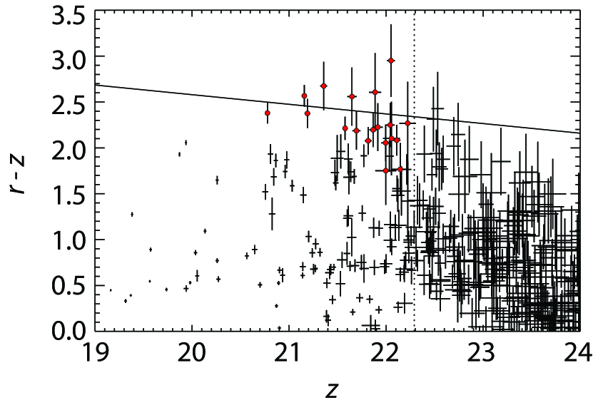
Photometric redshifts based on the cluster red-sequence were measured from both optical and IRAC color magnitude relations, shown in Figure 2. The best-fit photometric redshift in both cases is consistent with . We have used this value in converting the observed SZ decrement to a total mass.
3. Analysis
3.1. Identification of Compact Radio Sources
Compact radio sources are a potential source of uncertainty in SZ cluster mass measurements. Since these synchrotron sources are often variable, it is important to identify and remove their contribution contemporaneously with the SZ measurement. The long baselines of our CARMA observations (up to 12 k) can identify compact emission sources at high sensitivity. We identify contaminating sources by visual inspection of the long-baseline data and checking the 1.4 GHz catalogs from the NRAO VLA Sky Survey (NVSS, Condon et al., 1998) and the VLA Faint Images of the Radio Sky at Twenty-Centimeters (FIRST, Becker et al., 1995). A radio source is jointly modeled with the cluster signal if its flux is detected in the CARMA data at 3 or greater, or if there is a source in the NVSS or FIRST catalog. In the case that the source is only marginally-detected in the CARMA data and present in a VLA catalog, its position is fixed and only the flux is allowed to vary. The simultaneous fit mitigates the contamination of our significance and mass fits due to variable emissive sources, as described below.
In MOO J11553901, which has a centrally located source of emission detected at in the CARMA data, there exists a slight positive correlation between the measured parameter for the cluster and the point source flux. In the remaining 4 clusters, there is no sign of covariance between the cluster parameters and other source parameters. The coordinates and beam-corrected fluxes of compact radio sources identified toward each cluster are given in Table 2.
3.2. SZ Decrement Significance
To determine the significances of the observed SZ decrements, we measure the difference in between a model of our observations that contains no cluster with models (described in §3.3) that do include a cluster. In the cases where there is contaminating radio emission, models for these point sources are fitted in both the cluster and no-cluster models. The models are fit to the data in the -plane using a Markov chain Monte Carlo routine, which correctly accounts for the noise in our data from the heterogeneous CARMA array (see, e.g., Plagge et al., 2013).
The resulting values are converted to significances in terms of Gaussian standard deviations. They range from 2.7 to 9.5 and are listed in Table 3. In fitting the SZ cluster centroids, a uniform 1.5′ radius prior centered on the IR position is used. For low significance decrements, negative noise spikes can formally bias the SNR to higher values. However, given the strong prior of an IR-selected, confirmed cluster at the targeted position, and the small number of independent beams () over which the SZ centroid is allowed to vary, we expect all of these decrements to be robust. Using an approximate analytical calculation of the noise properties in our CARMA maps we conservatively estimate the probability of false detection for the two least significant clusters to be 8-10%. The higher significance clusters have no significant probability of false detection.
3.3. SZ Mass Measurements
The mass estimates are produced following the method described in recent CARMA papers (e.g. Brodwin et al., 2012). Briefly, we parameterize the SZ signal as a pressure profile that we integrate to measure the integrated Compton parameter. We use a generalized NFW pressure profile as presented in Nagai et al. (2007),
| (1) |
where is the normalization, is a dimensionless radial variable, and and are allowed to vary. The power-law exponents are fixed to the “universal” values (i.e., , , and ) of Arnaud et al. (2010). The cluster centroid and the positions and fluxes of any coincident emissive sources are allowed to vary as well. There is a strong degeneracy between and in the data, however the resulting parameter, as defined below, is well-constrained.
We integrate the derived pressure profile to a cutoff radius to calculate the integrated parameter,
| (2) |
To determine the cutoff radius, we enforce consistency with the scaling relation derived in Andersson et al. (2011) by requiring that the chosen integration radius (and thus, mass) and resulting lie on the mean relation. We determine the final integration radius iteratively, and the value of typically converges in roughly five iterations. The values in Table 3 correspond to the derived values of in our cosmology.
| ID | Redshift | Significance | 11 masses were extrapolated from the measured masses using the Duffy et al. (2008) mass–concentration relation. | 22 is the offset between the IR and SZ positional centroids. | |||
|---|---|---|---|---|---|---|---|
| () | (Mpc) | ( Mpc2) | ( ) | ( ) | (Mpc) | ||
| MOO J00121602 | 0.944 | 2.7 | 0.270 | ||||
| MOO J03190025 | 1.194 | 6.6 | 0.194 | ||||
| MOO J10140038 | 33The fit for this cluster assumed a Gaussian redshift prior with centered on the photometric redshift of . Due to the flat angular diameter distance, the redshift independence of the SZ and the narrow evolutionary window, no scatter is imposed by the redshift uncertainty at the significance presented. | 9.5 | 0.142 | ||||
| MOO J11553901 | 1.009 | 2.8 | 0.099 | ||||
| MOO J15141346 | 1.059 | 3.2 | 0.282 |
3.4. SZ and IR Centroids
The SZ and IR galaxy density centroids trace different physical probes of the potential, namely the integrated pressure of the ICM and the distribution of massive galaxies, respectively. For individual clusters these need not be coincident. Indeed, recent work has suggested that even X-ray and SZ centroids may be offset from each other during a major merger (Zhang et al., 2014).
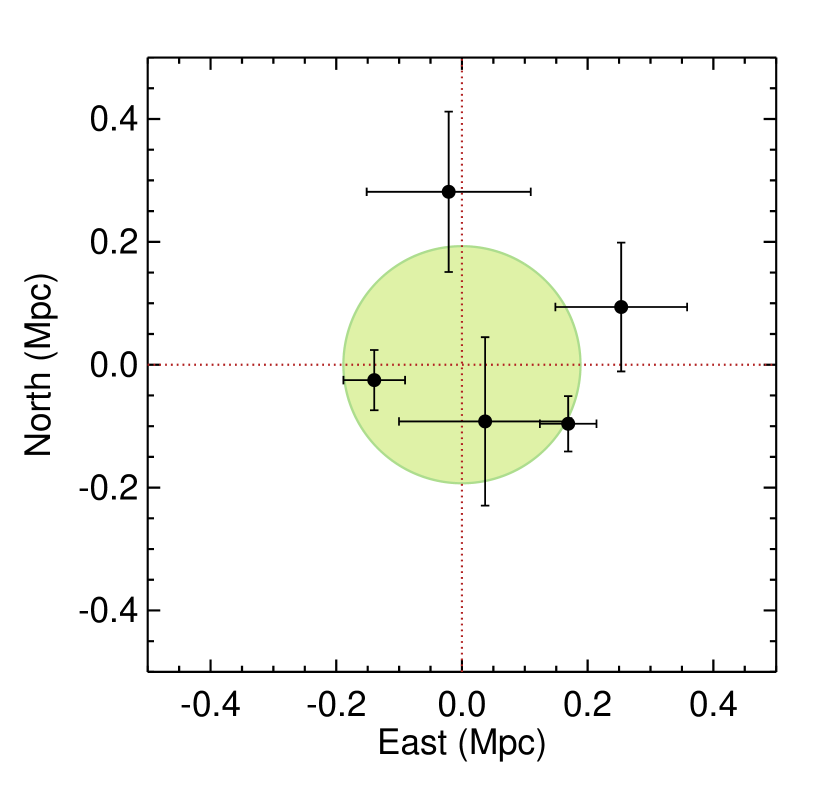
In Figure 3 we plot the angular offsets of the CARMA SZ cluster centroids from the WISE IR cluster positions, taken as the peaks in the wavelet detection map. The SZ-IR offset is less than 300 kpc for all the clusters in this sample. The error bars represent the quadrature sum of the uncertainties in the CARMA and WISE centroids. The CARMA positional errors, , determined in the fit described in §3.3, are jointly fit with the positions and fluxes of the emissive radio sources. The WISE centroiding precision is limited by finite gridding (15″/pixel) in the WISE cluster search, and to a lesser extent, to confusion caused by the relatively large WISE beam (). However, the metric offsets caused by these technical factors should be small ( kpc) for these high-SNR cluster detections.
The larger offsets seen here are likely due to real differences between IR galaxy density and SZ ICM centroids. We estimate the average residual positional offset, , by setting the reduced chi-squared statistic equal to unity:
| (3) |
where is the number of degrees of freedom. We find kpc, shown as the filled circular region at the center of the plot. A similar result is obtained using IR centers defined by the BCGs identified in follow-up IRAC imaging, confirming the IR-SZ offset is not due to an unknown systematic in the WISE centering.
4. Discussion
We have presented SZ decrements and derived masses for five distant (), massive ( ) MaDCoWS galaxy clusters selected via their stellar mass signatures in the WISE All-Sky data release. Four of these are spectroscopically confirmed (Stanford et al., 2014), and we have presented a reliable photometric redshift for the fifth derived from both deep optical and Spitzer photometry.
The current MaDCoWS catalog is drawn from the 10,000 deg2 overlap between the WISE and SDSS surveys. With the largest volume yet surveyed at high redshift, we expect to find very rare, massive clusters in the distant Universe. Indeed, three of the clusters in this preliminary CARMA pilot study have masses in excess of , among the most massive discovered to date at . More extensive characterization of the MaDCoWS sample is underway with CARMA and other facilities, including an ongoing AO-13 XMM-Newton program targeting several of the clusters presented in this work.
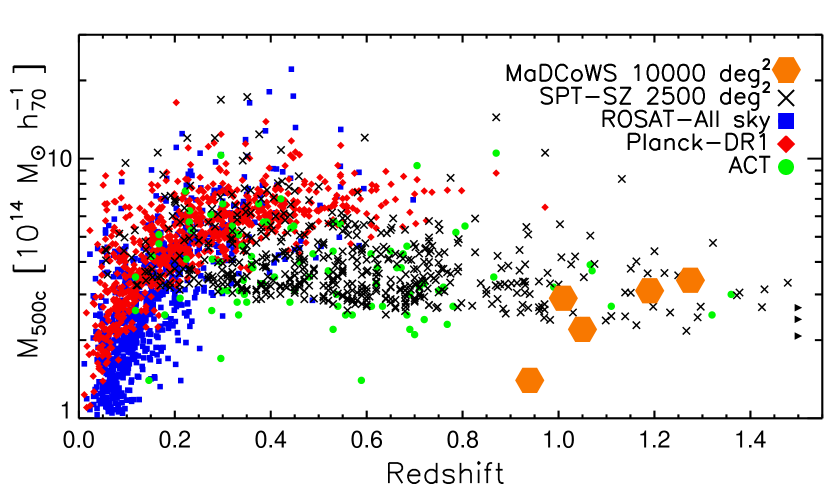
Figure 4, adapted from Bleem et al. (2015), shows the mass–redshift plane for the largest, wide-area cluster surveys to date. These include the ROSAT X-ray surveys (Piffaretti et al., 2011), composed of the NORAS (Böhringer et al., 2000), REFLEX (Böhringer et al., 2004) and MACS (Ebeling et al., 2001, 2007, 2010) cluster catalogs, and the SZ cluster catalogs from the Planck (Planck Collaboration et al., 2014), ACT (Marriage et al., 2011; Hasselfield et al., 2013) and SPT (Reichardt et al., 2013; Bleem et al., 2015) collaborations. The IR-selected MaDCoWS clusters presented in this work, shown as orange hexagons, are similar to the high-redshift clusters selected from the high-resolution SZ surveys (i.e., SPT and ACT). They are drawn from the massive cluster population at , and as ICM and/or weak lensing masses for the larger MaDCoWS sample are measured, we should identify high-redshift () clusters even more massive than those seen to date in the smaller-area SZ surveys.
In the near future, the MaDCoWS sample will be extended in both area and redshift. The recent AllWISE data release (Cutri, 2013) has significantly more uniform sky coverage, with an average of twice the exposure time over the previous all-sky catalog. This should allow the identification of massive galaxy clusters to . Our current search is also limited to the SDSS footprint. With the arrival of large optical surveys in, or extending to, the Southern hemisphere, such as Pan-STARRS, VST and DES, our search area will soon cover the bulk of the extragalactic sky. This will enable the discovery, within MaDCoWS, of the rarest, most massive clusters at .
References
- Aihara et al. (2011) Aihara, H., et al. 2011, ApJS, 193, 29
- Andersson et al. (2011) Andersson, K., et al. 2011, ApJ, 738, 48
- Arnaud et al. (2010) Arnaud, M., Pratt, G. W., Piffaretti, R., Böhringer, H., Croston, J. H., and Pointecouteau, E. 2010, A&A, 517, A92
- Bayliss et al. (2014) Bayliss, M. B., et al. 2014, ApJ, 794, 12
- Becker et al. (1995) Becker, R. H., White, R. L., and Helfand, D. J. 1995, ApJ, 450, 559
- Bleem et al. (2015) Bleem, L. E., et al. 2015, ApJS, 216, 27
- Böhringer et al. (2004) Böhringer, H., et al. 2004, A&A, 425, 367
- Böhringer et al. (2000) Böhringer, H., et al. 2000, ApJS, 129, 435
- Brodwin et al. (2012) Brodwin, M., et al. 2012, ApJ, 753, 162
- Brodwin et al. (2010) Brodwin, M., et al. 2010, ApJ, 721, 90
- Brodwin et al. (2013) Brodwin, M., et al. 2013, ApJ, 779, 138
- Condon et al. (1998) Condon, J. J., Cotton, W. D., Greisen, E. W., Yin, Q. F., Perley, R. A., Taylor, G. B., and Broderick, J. J. 1998, AJ, 115, 1693
- Cutri (2013) Cutri, R. M. 2013, VizieR Online Data Catalog 2328, 0
- Dressler et al. (2006) Dressler, A., Hare, T., Bigelow, B. C., and Osip, D. J. 2006, in Society of Photo-Optical Instrumentation Engineers (SPIE) Conference Series, Presented at the Society of Photo-Optical Instrumentation Engineers (SPIE) Conference
- Duffy et al. (2008) Duffy, A. R., Schaye, J., Kay, S. T., and Dalla Vecchia, C. 2008, MNRAS, 390, L64
- Ebeling et al. (2007) Ebeling, H., Barrett, E., Donovan, D., Ma, C.-J., Edge, A. C., and van Speybroeck, L. 2007, ApJ, 661, L33
- Ebeling et al. (2001) Ebeling, H., Edge, A. C., and Henry, J. P. 2001, ApJ, 553, 668
- Ebeling et al. (2010) Ebeling, H., Edge, A. C., Mantz, A., Barrett, E., Henry, J. P., Ma, C. J., and van Speybroeck, L. 2010, MNRAS, 407, 83
- Eisenhardt et al. (2008) Eisenhardt, P. R. M., et al. 2008, ApJ, 684, 905
- Fassbender et al. (2011a) Fassbender, R., et al. 2011a, New J. Phys., 13, 125014
- Fassbender et al. (2011b) Fassbender, R., et al. 2011b, A&A, 527, L10
- Galametz et al. (2010) Galametz, A., Stern, D., Stanford, S. A., De Breuck, C., Vernet, J., Griffith, R. L., and Harrison, F. A. 2010, A&A, 516, A101
- Gettings et al. (2012) Gettings, D. P., et al. 2012, ApJ, 759, L23
- Gonzalez et al. (2012) Gonzalez, A. H., et al. 2012, ApJ, 753, 163
- Hasselfield et al. (2013) Hasselfield, M., et al. 2013, JCAP, 7, 8
- Marriage et al. (2011) Marriage, T. A., et al. 2011, ApJ, 737, 61
- Mehrtens et al. (2012) Mehrtens, N., et al. 2012, MNRAS, 423, 1024
- Muchovej et al. (2007) Muchovej, S., et al. 2007, ApJ, 663, 708
- Mullis et al. (2005) Mullis, C. R., Rosati, P., Lamer, G., Böhringer, H., Schwope, A., Schuecker, P., and Fassbender, R. 2005, ApJ, 623, L85
- Muzzin et al. (2013) Muzzin, A., Wilson, G., Demarco, R., Lidman, C., Nantais, J., Hoekstra, H., Yee, H. K. C., and Rettura, A. 2013, ApJ, 767, 39
- Muzzin et al. (2009) Muzzin, A., et al. 2009, ApJ, 698, 1934
- Nagai et al. (2007) Nagai, D., Kravtsov, A. V., and Vikhlinin, A. 2007, ApJ, 668, 1
- Newman et al. (2014) Newman, A. B., Ellis, R. S., Andreon, S., Treu, T., Raichoor, A., and Trinchieri, G. 2014, ApJ, 788, 51
- Papovich et al. (2010) Papovich, C., et al. 2010, ApJ, 716, 1503
- Piffaretti et al. (2011) Piffaretti, R., Arnaud, M., Pratt, G. W., Pointecouteau, E., and Melin, J.-B. 2011, A&A, 534, A109
- Plagge et al. (2013) Plagge, T. J., et al. 2013, ApJ, 770, 112
- Planck Collaboration et al. (2014) Planck Collaboration, Ade, et al. 2014, A&A, 571, A29
- Reichardt et al. (2013) Reichardt, C. L., et al. 2013, ApJ, 763, 127
- Rettura et al. (2014) Rettura, A., et al. 2014, ApJ, 797, 109
- Rosati et al. (2004) Rosati, P., et al. 2004, AJ, 127, 230
- Rudy et al. (1987) Rudy, D. J., Muhleman, D. O., Berge, G. L., Jakosky, B. M., and Christensen, P. R. 1987, Icarus, 71, 159
- Santos et al. (2011) Santos, J. S., et al. 2011, A&A, 531, L15
- Sault et al. (1995) Sault, R. J., Teuben, P. J., and Wright, M. C. H. 1995, in R. A. Shaw, H. E. Payne, & J. J. E. Hayes (ed.), Astronomical Data Analysis Software and Systems IV, Vol. 77 of Astronomical Society of the Pacific Conference Series, p. 433
- Song et al. (2012) Song, J., et al. 2012, ApJ, 761, 22
- Stanford et al. (2012) Stanford, S. A., et al. 2012, ApJ, 753, 164
- Stanford et al. (2014) Stanford, S. A., Gonzalez, A. H., Brodwin, M., Gettings, D. P., Eisenhardt, P. R. M., Stern, D., and Wylezalek, D. 2014, ApJS, 213, 25
- Stanford et al. (2006) Stanford, S. A., et al. 2006, ApJ, 646, L13
- Willis et al. (2013) Willis, J. P., et al. 2013, MNRAS, 430, 134
- Wright et al. (2010) Wright, E. L., et al. 2010, AJ, 140, 1868
- Zeimann et al. (2013) Zeimann, G. R., et al. 2013, ApJ, 779, 137
- Zeimann et al. (2012) Zeimann, G. R., et al. 2012, ApJ, 756, 115
- Zhang et al. (2014) Zhang, C., Yu, Q., and Lu, Y. 2014, ApJ, 796, 138