Lagrangian analysis of the vertical structure of eddies
simulated in the Japan Basin of the Japan/East Sea

Abstract

The output from an eddy-resolved multi-layered circulation model is used to analyze the vertical structure of simulated deep-sea eddies in the Japan Basin of the Japan/East Sea constrained by bottom topography. We focus on Lagrangian analysis of anticyclonic eddies, generated in the model in a typical year approximately at the place of the M3 mooring (Takematsu et al., 1999) and the hydrographic sections (Talley et al., 2001), where such eddies have been regularly observed in different years (1993–1997, 1999–2001). Using a quasi-3D computation of the finite-time Lyapunov exponents and displacements for a large number of synthetic tracers in each depth layer, we demonstrate how the simulated feature evolves of the eddy, that does not reach the surface in summer, into a one reaching the surface in fall. This finding is confirmed by computing deformation of the model layers across the simulated eddy in zonal and meridional directions and in the corresponding temperature cross sections. Computed Lagrangian tracking maps allow to trace the origin and fate of water masses in different layers of the eddy. The results of simulation are compared with observed temperature zonal and meridional cross sections of a real anticyclonic eddy to be studied at that place during the oceanographic Conductivity, Temperature, and Depth (CTD) hydrochemical survey in summer 1999 (Talley et al., 2001). Both the simulated and observed eddies are shown to have the similar eddy core and the relief of layer interfaces and isotherms.

1 Introduction

The Japan/East Sea (JES) is the semi-closed marginal sea with narrow shallow straits and three deep basins. The Proper Water of the JES with a weak stratification is formed from the surface waters basically during winter in the deepest Japan Basin (JB, 3000–3560 m). It occupies the northern part of the sea (Fig. 1) where the climate is more severe than in the southern one. The general circulation pattern of the JES, to be found from observations (see, e. g., Takematsu et al., 1999; Lee and Niiler, 2005, and references therein) and modeling (see, e. g., Holloway et al., 1995; Yoon and Kim, 2009, and references therein), includes the cyclonic gyre with several cores of the large-scale cyclonic patterns over the JB (see, e. g., Trusenkova and Ishida, 2005, and references therein) and a current system with prevailing anticyclonic vorticity in the southern sea area (see, e. g., Lee and Niiler, 2005, 2010, and references therein).

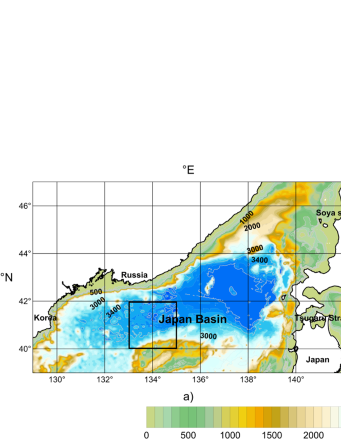
Figure 1: The bottom topography in a) the northern part of the Japan/East Sea and b) the studied area.

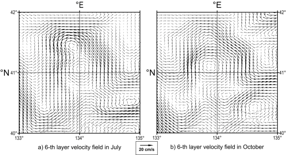
Figure 2: Simulated current velocity field in the studied area in the 6th layer velocity field averaged over a) July and b) October.

The Subpolar Front (SPF) separates subtropical and subarctical waters and lies between $38^{\circ}\,\text{N}$ and $41^{\circ}\,\text{N}$ being a boundary of distinct physical and chemical properties and a distinct vertical water structure (Talley et al., 2006). The zonal eastward current along the SPF is known to be highly variable with seasonal migration (Yoon and Kim, 2009). Meandering of the SPF is accompanied with formation of eddies of different polarity and sizes generated through baroclinic instability (Lee and Niiler, 2005, 2010). Satellite infrared images and drifter observations show that the eastward extension of the East Korean Warm Current along the SPF looks like a typical frontal eddy street (the scale is about 100 km) over the southern edge of the JB. The mesoscale and submesoscale eddies with smaller scales 30–50 km and 3–10 km are formed, respectively, over the JB and its steep northwestern continental slope and shelf break (Prants et al., 2011a, 2013b).

Anticyclonic eddies have been often observed to the north of the SPF. As part of an international cooperative program Circulation Research of the East Asian Marginal Seas (CREAMS), long-term moored current measurements have been carried out at seven sites in the JB. One of the moorings, M3, was deployed at $41.5^{\circ}\,\text{N}$ and $134.3^{\circ}\,\text{E}$ where the JB is 3500 m deep. It was equipped with three current meters at about 1000, 2000 and 3000 m depths which made the measurements for three years, from August 1993 to July 1996, with the data sampling period of one hour. The current meter data of 3-year duration have shown that deep-sea anticyclonic eddies (ACEs) with the orbital speeds of the order of 0.1 m s^-1 occurred every year in the deep layers (Takematsu et al., 1999). Available time series of sea-surface-temperature images and World Ocean Circulation Experiment (WOCE) drifter tracks were well correlated to that finding. The currents at 1000, 2000, 3000 m have been found by (Takematsu et al., 1999) to be highly coherent throughout the observational period of August 1993 to July 1996. They have observed intensification of the current in fall and winter. The eddies observed in the JB did not exhibit any definite direction of propagation. (Takematsu et al., 1999) indicated that the effect of the bottom geometry may be important. Once a barotropic eddy is established in the JB, it will be forced to remain only in the interior region of the Basin. In fact, the eddy currents were observed only at M3, but not in the rim area of the Basin at M1, M2, M4, M6 and M7 stations (Takematsu et al., 1999).

During the oceanographic CTD-hydrochemical survey in summer 1999 (Talley et al., 2001, 2006), the mesoscale ACE with the center approximately at the site of the M3 mooring has been found in temperature, salinity, dissolved oxygen and NO₃ sections along $134^{\circ}\,\text{E}$ and $41.25^{\circ}\,\text{N}$.

In this paper we use the output from the eddy-resolved multi-layered circulation MHI model (Shapiro, 2000) to analyze from a Lagrangian perspective the vertical structure of simulated deep-sea ACEs in the JB constrained by bottom topography. We focus on the ACE, generated in the MHI model approximately at the place of the M3 mooring (Takematsu et al., 1999) and the hydrographic sections (Talley et al., 2001, 2006), where such eddies have been regularly observed in different years (1993–1997, 1999–2001).

Two-dimensional Lagrangian approach has been successfully applied for studying horizontal transport and mixing in numerically-generated and altimetric velocity fields in different basins, from bays (Lekien et al., 2005; Lipphardt et al., 2006; Gildor et al., 2009; Prants et al., 2013b) and seas (Abraham and Bowen, 2002; d’Ovidio et al., 2004; Schneider et al., 2005; Mancho et al., 2008; Prants et al., 2013a) to the ocean scale (Beron-Vera et al., 2008; Waugh and Abraham, 2008; Prants, 2013; Prants et al., 2014c). Lagrangian methods are especially suitable because they allow to delineate eddy’s boundaries (Prants et al., 2011a; Beron-Vera et al., 2013; Prants et al., 2014c), to visualize transport barriers and corridors along which the core of an eddy is exchanged by water with its surrounding (Sulman et al., 2013; Prants et al., 2013b, a) and to quantify that transport (Miller et al., 1997).

The challenging problem is identifying the vertical structure of an eddy and quantifying its coherence. In order to quantify properties of the 3D structure of eddies (for example, their volume), it is often the eddy’s surface edges are simply extended to a given depth along the vertical. It is well known, however, that most eddies do not have a cylinder-like form. Moreover, the intriguing problem is changes in the structure of eddies at different depths in the course of time.

The Lagrangian analysis in this paper will be performed using two indicators, the finite-time Lyapunov exponent (FTLE) (Pierrehumbert and Yang, 1993) and displacements for a large number of tracers (Prants et al., 2011b; Prants, 2013; Prants et al., 2014c). We will show how our modeled ACE evolves of the eddy without any signs of rotation motion at the sea surface in summer into a one reaching the surface in fall. In order to demonstrate that we implement a quasi-3D computation of those Lagrangian indicators. We use the full 3D velocity field from the output of the MHI model and compute the synoptic maps of the FTLE and particle’s displacements in every model layer.

Quasi-3D Lagrangian approach has been applied recently by (Bettencourt et al., 2012) for diagnostics of 3D Lagrangian coherent structures around a particular cyclonic eddy pinched off from a Benguela upwelling front. Three-dimensional Lagrangian coherent structures were extracted as “ridges” of the calculated fields of the finite-size Lyapunov exponent obtained from an output of the Regional Ocean Modeling System (ROMS). They have been found by (Bettencourt et al., 2012) to be quasi-vertical surfaces. Another eddy feature, a ring of the Loop Current in the Gulf of Mexico has been studied by (Sulman et al., 2013) by the similar method, using the data-assimilating HYbrid Coordinate Ocean Model (HYCOM). Those authors have studied the location of relevant transport barriers during the formation of Eddy Franklin in 2010 at several depths from the surface down to 200 m.

Our paper is organized as follows. Section 2 describes briefly the eddy-resolved multi-layered circulation MHI model adopted to the JES and the Lagrangian approach to be used. Section 3 contains the main results of the 3D Lagrangian analysis of isolated deep-sea eddies in the JB. As the study case, we focus on a simulated mesoscale ACE to the north of the SPF and investigate its vertical structure. Backward-in-time FTLE and drift maps are calculated in different layers in Section 3.1 to illustrate the evolution of boundaries of the eddy and its vertical structure during summer and fall. The deformation of the model layers across the eddy in zonal and meridional directions and the corresponding temperature cross sections are computed in Section 3.2 and compared in Section 3.3 with the data of the oceanographic CTD-hydrochemical survey in summer 1999 (Talley et al., 2001, 2006). In Section 3.4 we calculate the Lagrangian tracking maps which allow to illustrate pathways and barriers to transport into and out of the eddy at different depths. The form, nonlinearity and stability of simulated ACEs are discussed briefly in the end of Section 3.

2 The model and methods

2.1 Circulation numerical model adopted to the Japan/East Sea

We use the MHI ocean circulation quasi-isopicnal layered model (Mikhailova and Shapiro, 1993; Shapiro, 2000) with a free surface boundary condition incorporating the horizontally inhomogeneous upper mixed layer. The model is based on a system of primitive equations integrated within each quasi-isopicnal layer. All layers are assumed to be horizontally inhomogeneous, however, the density in each thermocline layer changes within the limits determined a priori by the prescribed basic stratification.

It is assumed that the layers may outcrop. The layer outcropping is similar to the isopycnal model applied by (Hogan and Hurlburt, 2006) to the Japan/East Sea. The interfaces of the inner model layers can climb to the upper mixed layer in the frontal zones. The horizontally inhomogeneous upper-mixed-layer model includes parametrizations of turbulent heat, salt and momentum fluxes, drift current in that layer, entrainment and subduction processes at the bottom of the layer (Mikhailova and Shapiro, 1993; Shapiro, 2000). The basic equations for momentum, temperature and salinity in the upper mixed layer are similar to the integrated vertically equations for inner layers of the model. The commonly used convective adjustment scheme is applied to simulate vertical convection. According to our previous studies (Prants et al., 2011a) the MHI quasi-isopycnal layered model successfully simulates the mesoscale eddy dynamics, interaction between eddies over the shelf edge and steep continental slope of the Japan Basin, as well as, mesoscale eddies and currents, mixing and transport of water masses in the Peter the Great Bay of the Japan/East Sea (Prants et al., 2013b).

The numerical experiment with the MHI model is focused in this paper on simulation of the mesoscale circulation over the deep JB, its continental slope and shelf during summer and fall. The model domain is the closed sea area $39\text{--}44^{\circ}\,\text{N}$ and $129\text{--}139^{\circ}\,\text{E}$ with the horizontal resolution 2.5 km (Prants et al., 2011a).

The no-slip boundary conditions for current velocity at the sea domain contour, including sea coast, northern, eastern and southern boundaries, are set. The model is assumed to consist of 10 quasi-isopycnal layers with the first one to be a horizontally inhomogeneous upper mixed layer. The first 9 layers are located inside the main pycnocline with the lower boundary of the ninth layer to be the lower boundary of the main pycnocline which is not deeper than 250 m in the area studied. The lower tenth layer includes deep and bottom waters of the JES. The realistic bottom topography (Fig. 1), obtained from ETOPO2 (2-Minute Gridded Global Relief Data), is one of the most important factor in simulation of the large scale and mesoscale circulations.

The initial conditions for summer isopycnal interfaces in the model layers, temperature and salinity distribution include only large scale features of the model variables. It have been taken from oceanographic survey in 1999 (Talley et al., 2001, 2006) with a substantial smoothing. After smoothing, there were no any mesoscale structures in the initial conditions. The MHI model has been integrated with the time step of 4 min from the initial condition under realistic meteorological situations. The first month with June meteorological conditions is a time interval of the model spin up. The wind stress, short wave radiation, near surface air temperature, humidity and wind speed have been taken from daily mean National Centers for Environmental Prediction/National Center for Atmospheric Research (NCEP/NCAR) Reanalysis. The heat fluxes at the sea surface, being depended on the mixed layer temperature and meteorological characteristics, are calculated in the model.

The coefficients of quasi-isopycnal biharmonic viscosity, harmonic viscosity, and diffusion used in the momentum and heat/salt transfer equations have been varied correspondingly from $10^{17}$ m⁴s^-1, $10^{7}$ m²s^-1 and $0.4\cdot 10^{7}$ m²s^-1 in the model spin up (60 days) to $10^{16}$ m⁴s^-1, $10^{6}$ m²s^-1 and $0.4\cdot 10^{6}$ m²s^-1 during the other months of the warm period of a year until late November. The quasi-isopycnal harmonic viscosity is applied only near the domain boundary in a warm period of a year and in the whole area in winter. We basically simulate the nonlinear large scale and mesoscale circulation over the JB, continental slope and shelf taking into account daily mean external atmospheric forcing from July 1 to December 1. The numerical experiments with minimized coefficients of the horizontal and vertical viscosity show intensive mesoscale dynamics. In particular, they demonstrate variability of the mesoscale anticyclonic and cyclonic eddies over the shelf, the shelf break and base of the continental slope and in the central deep area of the JB as well. The anticyclonic eddies, generated over the shelf break and continental slope, move usually downstream of the current with prevailing phase velocity of about 6–8 cm s^-1 (Prants et al., 2011a). Some quasi-stationary mesoscale eddies in the central JB area, including the eddies studied in this paper, are generated in the thermocline and deep JB water over the mesoscale bottom troughs and sea mounts.

Figure 2 demonstrates the monthly mean current velocity fields in July and October in the 6th model layer in the deep JB area (see Fig. 1 a). The system of anticyclonic and cyclonic eddies in the velocity field varies from July to October – November. The most stable one is an ACE simulated in the central region of the studied area over a mesoscale bottom trough. Its center is shifting with time during the model run from July to November in the vicinity of the point with coordinates $41.15^{\circ}\,\text{N}$ and $134^{\circ}\,\text{E}$ where similar ACEs have been often observed during the oceanographic survey in early August 1999 (Talley et al., 2001, 2006) and in the current meter observation from August 1993 to July 1996 at the mooring station M3 (Takematsu et al., 1999). The mesoscale cyclonic eddies, surrounding the anticyclonic one, look like short-lived eddies moving around the anticyclone with the lifetime of about a few days.

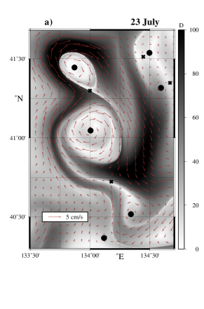
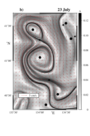
Figure 3: Manifestations of modeled eddies on 23 July in the ninth layer on a) the drift map ($D$ in km) and b) the Lyapunov map ($\Lambda$ is in days^-1) with the velocity field imposed. “Instantaneous” elliptic and hyperbolic points, to be present in the area on 23 July, are indicated by circles and crosses, respectively.

2.2 Lagrangian approach

Two-dimensional motion of a fluid particle inside each modeled layer is governed by advection equations

$$\frac{dx}{dt}=u(x,y,t),\quad\frac{dy}{dt}=v(x,y,t),$$ (1)

where $x$ and $y$ are the longitude and latitude of the particle, $u$ and $v$ are angular zonal and meridional components of its velocity inside a given layer. Numerically generated velocity fields are given as discrete data sets on a grid. So, a bicubical interpolation in space and an interpolation by third order Lagrangian polynomials in time are used to integrate Eqs. 1. The velocity components are interpolated independently on each other. The velocities obtained are substituted in Eqs. 1 which are integrated with a fourth-order Runge-Kutta scheme with a fixed time step. The outputs are transformed in the geographical coordinates to get images and maps.

A method for computing FTLE, which is valid for $n$-dimensional vector fields, has been proposed recently by (Prants et al., 2011a). The Lyapunov exponents in this method are defined via singular values, $\sigma_{i}(t,t_{0})$, of the evolution matrix for linearized $n$-dimensional equations of motion as follows:

$$\Lambda_{i}=\lim_{t\to\infty}\frac{\ln\sigma_{i}(t,t_{0})}{t-t_{0}},\quad i=1,2,\dots,n.$$ (2)

Quantities

$$\Lambda_{i}(t,t_{0})=\frac{\ln\sigma_{i}(t,t_{0})}{t-t_{0}}$$ (3)

are called FTLE which of each is the ratio of the logarithm of the maximal possible stretching in a given direction to a finite time interval $t-t_{0}$.

Synoptic maps of some Lagrangian indicators have been shown to be a useful means to visualize oceanic features over different scales like common hydrological and Lagrangian fronts (Prants, 2013; Prants et al., 2014b, a), strong currents (Prants et al., 2014c), submesoscale and mesoscale eddies (Prants et al., 2011a, 2013a). Such maps are obtained by integrating advection equations (1) backward in time for a given period, computing one of the Lagrangian indicators for a large number of tracers and coding its magnitude by color. The Lagrangian indicators are functions of particle’s trajectories which carry an information about origin and history of water masses.

The convenient Lagrangian indicator for identifying boundaries of submesoscale and mesoscale eddies is a finite-time absolute displacement, $D$, that is simply the distance between the final, $(x_{f},y_{f})$, and initial, $(x_{0},y_{0})$, positions of advected particles on the Earth sphere with the radius $R$

$$D\equiv R\arccos[\sin y_{0}\sin y_{f}+\cos y_{0}\cos y_{f}\cos(x_{f}-x_{0})].$$ (4)

This quantity along with zonal and meridional displacements have been shown to be useful in quantifying transport of radionuclides in the Northern Pacific after the accident at the Fukushima nuclear power plant in March 2011 (Prants et al., 2011b, 2014c) and in identifying Lagrangian fronts with favourable fishery conditions (Prants et al., 2014a).

3 Results of simulations

3.1 Three-dimensional structure and evolution of anticyclonic eddies in the Japan Basin

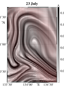
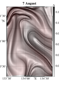
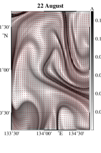
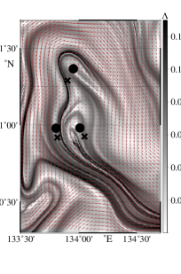
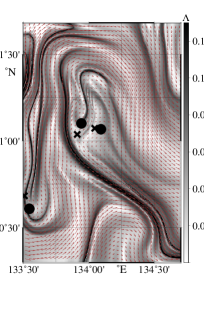
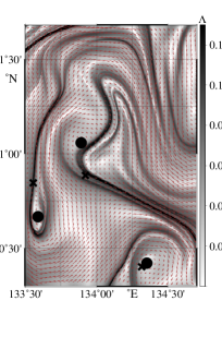
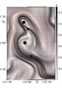
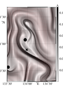
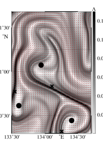
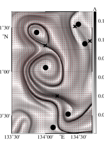
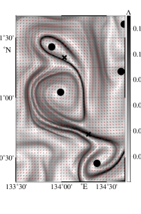
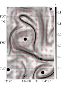
Figure 4: Vertical eddy structure in summer shown on 23 July, 7 and 22 August. The Lyapunov maps in the 1st, 3rd, 5th and 9th layers are shown from the top to the bottom, respectively. The vortex pair, seen in the lower layers, evolves gradually with time in a single eddy which, however, is not visible in the surface layers. The finite-time Lyapunov exponent $\Lambda$ is in units of days^-1. Elliptic and hyperbolic points are indicated by circles and crosses, respectively.

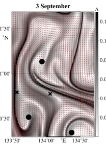
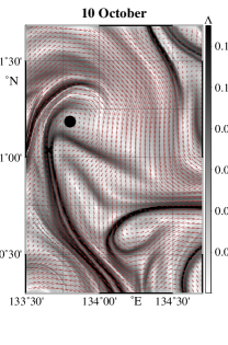
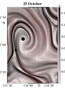
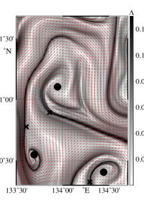
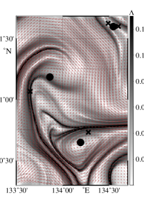
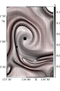
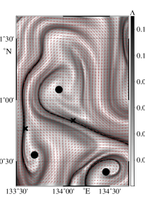
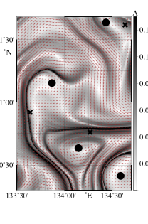
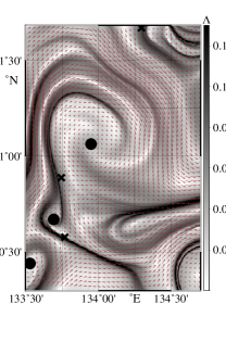
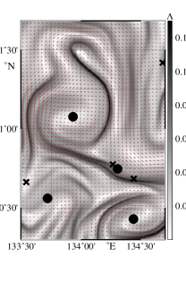
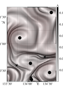
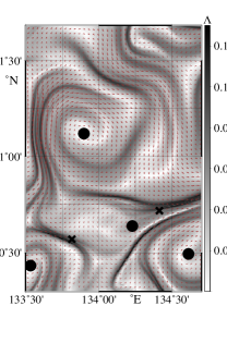
Figure 5: The same as in Fig. 4 but in fall on 3 September, 10 and 25 October. The eddy appears at the surface to the end of October.

In this section we focus on a simulated ACE centered at $\simeq 41^{\circ}\,\text{N}$ and $\simeq 134^{\circ}\,\text{E}$ which is visible in Fig. 2 in the 6th layer velocity field averaged over July and October in a typical year of simulation. It is a typical quasi-stationary coherent feature of the SPF, constrained by bottom topography (see the bathymetry map in Fig. 1b), that has been found in this area in satellite images (Takematsu et al., 1999) and measured at a mooring station (Takematsu et al., 1999) and in hydrographic surveys (Talley et al., 2001, 2006).

Eddy identification in our study is based on geometry of the velocity field and specific features of the FTLE and displacement fields. The following necessary and sufficient conditions we use to identify an eddy center and its boundaries. The velocity magnitude has zero value at the eddy center which is defined as an elliptic stagnation point whose stability is checked daily by the standard methods. The zonal and meridional rotational velocities have to reverse in sign across the eddy center, and their magnitudes have to increase initially away from it, go through a maximum and then decrease. Eddy boundaries are identified better in the FTLE and displacement fields than in the corresponding velocity field.

Eddy core and surrounding water masses may have a rather distinct origin that can be traced out with the help of so-called drift maps introduced by Prants et al. (2011b); Prants (2013); Prants et al. (2014c). The map for absolute displacements of tracers is computed as follows. A region under study is seeded with a large number of synthetic tracers for each of which advection equations are integrated backward in time for an appropriate period, 30 days in our case. The distance, $D$, between positions of each tracer on the first and last days of that period is calculated in each model layer as (4) and coded by color. Such a map in Fig. 3 a clearly demonstrates a vortex pair with two ACEs in the 9th layer with elliptic points at their centers ($41^{\circ}\,\text{N}$, $134^{\circ}\,\text{E}$) and ($41.4^{\circ}\,\text{N}$, $133.9^{\circ}\,\text{E}$) and a hyperbolic point in between ($41.3^{\circ}\,\text{N}$, $134^{\circ}\,\text{E}$). The boundary of the northern eddy core can be identified as a closed curve with the maximal local gradient of $D$ that separates waters, involved in the rotational motion around the vortex center, from ambient waters. Magnitudes of the absolute displacements for the former ones are much smaller than for the particles outside the eddy.

The southern eddy has a more complicated structure because of its intensive interaction with ambient waters during the month of integration. The drift maps allow to delineate the transport corridors by which eddies can gain water from their surroundings. They look like dark “tongues” in Fig. 3a encircling that eddy. The origin of those waters can be traced out by computing tracer’s displacements in zonal and meridional directions backward in time for the month, from 23 July to 23 June. The corresponding zonal and meridional drift maps shown in Fig. S1 allow to visualize where the waters in the ninth layer came from. Blue color of the water “tongues” around that eddy mean that it trapped waters from the south (Fig. S1a) and east (Fig. S1b). Complementary backward-in-time Lagrangian longitudinal (Fig. S2a) and latitudinal (Fig. S2b) drift maps show by color the longitudes and latitudes, respectively, from which tracers, initialized in the area on 23 June, came to their final positions on 23 July.

The sharp boundary between waters with high gradients of a Lagrangian indicator (e. g., the absolute displacement $D$) was called a “Lagrangian front” (Prants, 2013; Prants et al., 2014b). The Lagrangian fronts, encircling each of the eddies in the pair in Fig. 3a, can be identified by a narrow white stripe demarcating the curve with the maximal gradient of $D$. White color means that the corresponding particles have experienced very small displacements over the period of integration because they rotated around eddy’s centers. The sizes of the southern and northern eddies are estimated to be $\approx 35\times 45$ km and $\approx 20\times 20$ km, respectively.

The FTLE field provides complementary information on the horizontal eddy structure. We computed it in the same area by the method (Prants et al., 2011a) and coded the values of the FTLE, $\Lambda$, by color. The map in Fig. 3b demonstrates the same vortex pair surrounded by black “ridges” with local maximal values of $\Lambda$ which are known to approximate unstable manifolds of the hyperbolic trajectories in the region (Haller and Yuan, 2000). There are typically a number of hyperbolic trajectories around eddies in the ocean which are connected with the corresponding hyperbolic stagnation points marked by crosses on our Lagrangian maps. Each of which has its own unstable manifold that is manifested on backward-in-time FTLE maps as a black “ridge” (for a review on chaotic advection in the ocean see Wiggins, 2005; Koshel’ and Prants, 2006).

In oceanic flows trajectories and stagnation points can gain or lose hyperbolicity over time. It means, in particular, that hyperbolic stagnation points may appear and disappear in the course of time. Only those ones, which exist on 23 July, are shown in Fig. 3. As to the southern eddy, it is confined from the east and south by the S-like unstable manifold of the hyperbolic point located between the eddies in the vortex pair. Any unstable manifold influences strongly on adjacent fluid parcels. It is illustrated in Fig. S3, where we placed blue and rose patches with tracers near the S-like unstable manifold, and advected them forward in time for three and half months. Both the patches elongate along that manifold. The red patch was chosen in the center of the northern eddy and is shown in Fig. S3 to deform slightly in the course of time until the northern eddy begins to break down to the end of summer. The southern eddy is confined from the west by the unstable manifold of a hyperbolic point which disappeared to 23 July but existed before. The complicated pattern of the black “ridges” around the southern eddy in Fig. 3b confirms the conclusion about its intensive interaction with ambient waters.

To illustrate the vertical structure of the vortex pair and its evolution we show in Fig. 4 the summer FTLE maps in the first, third, fifth and ninth layers. On 23 July the pair with two ACEs, elliptic points at their centers and a hyperbolic point in between is clearly seen in the lower layers below the 4th one. The vortex pair is especially prominent in the 9th layer that is a lower boundary of the main pycnocline. It is not recognizable in the third layer and above where the corresponding hyperbolic point between the eddies disappears, but the elliptic points still exist at their places. The elliptic points are absent at the surface where there are no signs of vortex motion.

In the course of time the pattern changes. The pair gradually decays in the sense that the northern eddy merges with the southern one (compare the map on 7 August with the map on 22 August when the northern elliptic point disappears in the 9th layer). As to the other layers, it is seen that the northern elliptic point disappears earlier. It is possible to recognize to 22 August a single ACE with the size $\approx 40\times 50$ km in the 5th layer and below. Thus, we have got to the end of summer the ACE not reaching the surface.

Changes in the vertical vortex structure in September and October are shown in Fig. 5. The eddy in fall is clearly visible in the 5th layer and below as a single ACE of the same size as in August. As to the surface layers, a prominent eddy structure becomes visible there only to the end of October. In the beginning of September the elliptic point appears in the first layer at the place where the eddy is visible in the 5th layer and below, but the eddy cannot be clearly detectable on the corresponding Lyapunov maps. Thus, the bowl-shaped eddy is formed to the end of October. It penetrates from the surface to the bottom gradually decaying to the end of November.

3.2 Zonal and meridional layer interface and temperature vertical sections across the simulated eddy

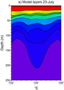
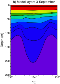
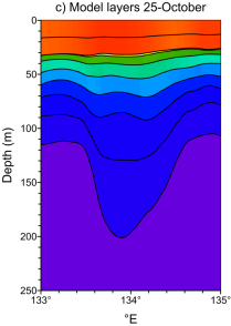
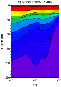
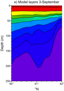
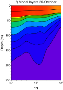
Figure 6: Zonal (along $41^{\circ}\,\text{N}$, the upper row) and meridional (along $134^{\circ}\,\text{E}$, the lower row) sections of the interfaces between modeled eddy layers on 23 July, 3 September and 25 October. Each quasi-isopycnal layer is shown by its own color.

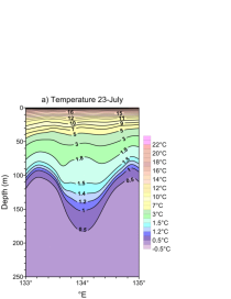
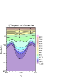
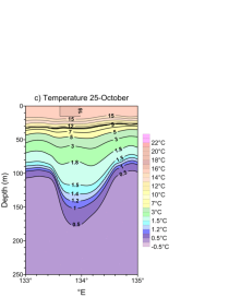
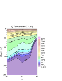
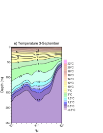
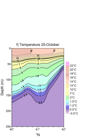
Figure 7: The same as in Fig. 6 but for temperature sections across the simulated eddy on 23 July, 3 September and 25 October.

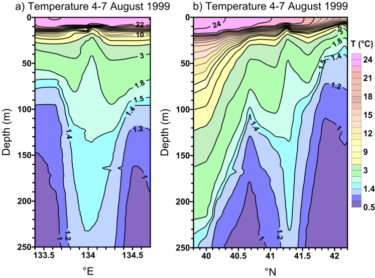
Figure 8: a) Zonal (along $41^{\circ}\,\text{N}$) and b) meridional (along $134^{\circ}\,\text{E}$) observed sections of temperature across the anticyclonic eddy to be found during the oceanographic CTD-hydrochemical survey in early August 1999 (Talley et al., 2001).

Ten layers have been used in the MHI model adopted to the JES. In order to illustrate transformation of our vortex structure with time, we compute vertical zonal and meridional sections across the simulated eddy. Figures 6 and 7 show evolution of its vertical structure from late July to late October in terms of sections of quasi-isopycnal layer interfaces (Fig. 6) and water temperature in the layers (Fig. 7). The anticyclonic eddy, illustrated on the Lagrangian maps in Figs. 3–5, is formed over the mesoscale bottom trough in early July at first in the main pycnocline and underlying layers and presents within the layers from the 4th one and below all the time after its formation.

The Lagrangian maps on 23 July in Fig. 3 clearly show the vortex pair oriented in the meridional direction. The zonal sections in Fig. 6 along the latitude $41^{\circ}\,\text{N}$ cross the southern ACE which is manifested as a depression of the layers from the 3rd to 9th ones around the elliptic point. The vortex pair evolves to 3 September to a single ACE (see Fig. 5) whose zonal cross section is shown in Fig. 6b. It still does not extend to the surface. To 25 October the eddy reaches the surface (see Figs. 5 and  6c). The northern ACE of the vortex pair, seen in Fig. 3 on 23 July, is hardly visible in the meridional cross section as a small depression in the lower layers to the right of the main depression (Figs. 6d and e).

From July to early September, the ACE presents only occasionally in the numerical solution in the upper mixed layer (layer 1) and in the seasonal pycnocline (layers 2–4). In this period of warm season, when the upper mixed layer is comparatively thin (see Figs. 6a, b, d and e) and the seasonal pycnocline is very strong (see Figs. 7a, b, d and e), the simulated ACE is unstable in the upper layers. Its lifetime in these layers does not exceed a few days. During summer, it episodically appears and breaks down into smaller submesoscale eddies in the upper layers. During October – November, when the thickness of the upper mixed layer increases from 10 to 15–30 m (Figs. 6c and f) and the seasonal pycnocline is weak, the ACE becomes as stable in the upper layers as in the underlying ones. It is also manifested in the zonal temperature section in Figs. 7c as the closed isotherm at the sea surface.

3.3 Zonal and meridional temperature vertical sections across the observed eddy

During the oceanographic CTD-hydrochemical survey in summer 1999 (Talley et al., 2001), the mesoscale ACE (with the center approximately at the same place as the M3 mooring (Takematsu et al., 1999) and our simulated eddy) has been observed in temperature, salinity, dissolved oxygen and NO₃ sections along $134^{\circ}\,\text{E}$ and $41.25^{\circ}\,\text{N}$. The warm fresh core of the eddy with high gradients in temperature, salinity and dissolved oxygen at its edge was situated in the thermocline within the layer from 50 to 150 m.

Figure 8 shows water temperature structure of that ACE in zonal and meridional sections of the oceanographic survey in early August 1999 (Talley et al., 2001). The density gradient in this eddy basically depends on the temperature gradient. The eddy core, to be surrounded by maximal temperature and density gradients, looks like a lens. The eddy occupies the water column below the seasonal pycnocline (30–50 m). The anticyclonic eddy was not clearly observed in the upper mixed layer and in the seasonal pycnocline both in the zonal and meridional temperature sections. It is an important feature of the observed eddy closely related to the simulation results discussed above. Eddies with similar vertical structure in temperature and density cross-sections, named as intra-thermocline eddies, have been observed south of the Subarctic Front over the western side of the Yamato Rise and within quasi-stationary meanders of the Tsushima Current (Gordon et al., 2002). They have been successfully simulated in this area by (Hogan and Hurlburt, 2006) using an isopycnal ocean circulation model. The observed eddy in Fig. 8 is situated over the mesoscale bottom trough surrounding by sea mounts in the western area of the JB (see Figs. 1a and b) practically in the same area as our simulated eddy. In summer, the position and the vertical structure of the simulated ACE in Figs. 6 and 7 are similar to those for the observed ACE in Fig. 8. Both the simulated and observed ACEs have the similar eddy core, the relief of layer interfaces and isotherms.

The observed ACE is stronger than the simulated one with a much more strong temperature/density front situated to the south of the ACE and a stronger vertical stratification. That difference may be explained by the fact that the observation has been made in the warm climatic period and warm year (1999), whereas the simulation has been performed under daily meteorological conditions averaged over 25-years period from 1976 to 2000. Moreover, we did not take into account meridional heat advection from the southern sea area and the southern boundary of the model domain due to no-slip boundary condition for the current velocity.

3.4 Tracking maps

Figure 9: Tracking maps for the markers distributed over the eddy’s core on 1 September in 1st, 5th, 7th, 9th and 10th layers numbered in the left lower corners. a) The forward-in-time map shows where the corresponding markers were walking from 1 September to 1 November. b) The backward-in-time map shows where they were walking from 1 September to 1 July. The density of traces is in the logarithmic scale.

In this section we apply a special Lagrangian technique (Prants et al., 2013b, 2014c) to visualize the origin and fate of water masses in the eddy core. A large number of markers (250 000) is distributed on 1 September in each layer around the eddy center inside the patch $7\times 11$ km ($133.87\text{--}133.97^{\circ}\,\text{E}$, $41\text{--}41.1^{\circ}\,\text{N}$). They are advected for two months backward and forward in time by the velocity field in each layer. The tracking maps are computed as follows. The region under study, $131\text{--}136^{\circ}\,\text{E}$ and $40\text{--}43.5^{\circ}\,\text{N}$ is divided in $500\times 500$ cells. One fixes each day which cells and how many times the markers have visited from 1 September to 1 July (backward-in-time tracking maps) and from 1 September to 1 November (forward-in-time tracking maps).

The results are shown in Fig. 9 and may be interpreted as follows. The forward-in-time tracking maps in Fig. 9a show where the corresponding markers in each chosen layer were walking from 1 September to 1 November. In this period, the markers from the patches in the lower layers, including the 5th one, rotated around the eddy center with an insignificant flow outside. The “tails” at the upper levels mean that at the surface the eddy expelled water from its periphery in different directions, however, preserving its core.

The backward-in-time tracking maps in Fig. 9b show where the corresponding markers in each chosen layer were walking from 1 September to 1 July. The patches with markers in the lower layers, from the 7th to 10th, practically did not change their form for two months in the past. It means that the eddy existed in those layers all that time at the same place without exchanging by the core water with its surroundings. The “tail” of the patch in the 5th layer means that the eddy in this layer gained the water from the south, but its core have been at the same place for the two months (see the FTLE maps in the 5th layer in Figs. 4 and 5). As to the surface layer (the upper plane in Fig. 9b), markers from the initial patch in the 1st layer came to their positions on 1 September from the west.

3.5 The form, nonlinearity and stability of simulated anticyclones

The ACE under study is an eddy-like feature in a region of the JB to the north of the Yamato Rise (see Fig. 1 a). That eddy has been found to be practically stationary for a half-year integration period including summer and fall. It is seen from the lower panels in Figs. 4 and 5 that displacement of its elliptic point for three months did not exceed 10 km. Inspection of the AVISO velocity field at the sea surface for 1992 – 2014 (http://www.aviso.oceanobs.com) has shown that surface eddy-like anticyclonic features often appeared in the area around ($\approx$ $134^{\circ}\,\text{E}$, $\approx$ $41^{\circ}\,\text{N}$) in cold seasons and disappeared in warm ones. No significant directed transport of such eddies has been found in those altimetric data. Taking into account these findings, complicted bottom topography in the area with underwater seamounts and trenches (see Fig. 1 b) and observations by (Takematsu et al., 1999), it is reasonably to suppose that we deal with the ACE constrained by bottom topography.

Computation of the FTLE and particle’s displacement in each depth layer clearly shows that the simulated ACE evolves of the eddy, that does not reach the surface in summer, into a one reaching the surface in fall. The corresponding elliptic points, demarcating the eddy’s center, are absent in upper layers in summer (Fig. 4) and appear in fall (Fig. 5). This finding is confirmed by computing deformation of the model layers and the temperature cross sections. Whether the eddy reaches the surface or not, it depends on the stratification measure in the thermocline, topographic and other parameters. In summer, when the upper mixed layer is comparatively thin and the stratification of seasonal pycnocline is very strong, the simulated eddy is unstable in the upper layers. In fall, when the stratification of seasonal pycnocline is much weaker than in summer, the eddy becomes as stable in the upper layers as in the underlying ones.

The eddy must be sufficiently nonlinear to exist as a stable entity. The measure of the nonlinearity is the so-called quasigeostrophic nonlinearity parameter $Q_{\beta}$, which is the ratio of the relative vorticity advection to the planetary vorticity advection (Chelton et al., 2011) defined as $Q_{\beta}=U/\beta L^{2}$, where $U$ is maximum rotational speed, $L$ the eddy radius and $\beta=df/dy$ is the planetary vorticity gradient. Let us estimate the quasigeostrophic nonlinearity parameter of our simulated eddy in the JB. Taking $U=0.05\text{--}0.1$ m s^-1, $L=30000$ m, $R^{2}=9\cdot 10^{8}$ m², and $\beta=1.73\cdot 10^{-11}$ m s^-1, one gets $Q_{\beta}=3.3\text{--}6.6$. This range of values means that the relative vorticity dominates and suggests that our simulated eddy is nonlinear and may persist as a coherent structure.

4 Conclusions

We numerically investigated the vertical structure of simulated mesoscale anticyclonic eddies often observed (Takematsu et al., 1999; Talley et al., 2001, 2006) to the north of the Subpolar Front in the Japan/East Sea. The model used for experiments was the MHI hydrothermodynamic quasi-isopycnal, eddy-resolved model of a multilayer ocean (Mikhailova and Shapiro, 1993; Shapiro, 2000) with the horizontal resolution of 2.5 km. The Lagrangian approach has been applied to study temporal evolution and a vertical structure of the anticyclonic vortex feature constrained by the bottom topography in the western area of the deep Japan Basin. The finite-time Lyapunov exponent field along with the field of tracer’s displacements have been shown to demarcate Lagrangian boundaries of the eddy, pathways and barriers organizing transport and mixing processes at the mesoscales and submesoscales.

Estimating the quasigeostrophic nonlinearity parameter of our modeled eddy, we have shown that it was sufficiently nonlinear to exist as a stable entity. The quasi-3D analysis has been performed in the period from July to November in a model period of a year when the eddy, visible in summer in the lower layers only, gradually changed its vertical structure to become visible in the surface layers in fall. In summer, when the upper mixed layer is comparatively thin and the seasonal pycnocline is very strong, the simulated eddy was shown to be unstable in the upper layers. During October – November, when the thickness of the upper mixed layer increases and the seasonal pycnocline is weak, that eddy becomes as stable in the upper layers as in the underlying ones. We applied a special tracking technique to find out transport pathways by which the eddy exchanged water with its surrounding at each depth level. It was found that at the surface the eddy gained and expelled water much more intensively than in the deep layers.

The results of simulation were compared with observed temperature zonal and meridional cross sections of a real anticyclonic eddy to be studied at that place during the oceanographic CTD-hydrochemical survey in summer 1999 (Talley et al., 2001, 2006). The position and the vertical structure of the simulated ACE have been found to be similar to those for the observed one. Both the simulated and observed eddies have the similar eddy core, the relief of layer interfaces and isotherms. The results of this paper would thus seem to indicate that topographically controlled eddies reaching the surface may be a state to which submerged eddies might evolve given sufficiently time.

Appendix A

Supplementary materials associated with this paper can be found in the online version.

References

- Abraham and Bowen (2002) Abraham, E.R., Bowen, M.M., 2002. Chaotic stirring by a mesoscale surface-ocean flow. Chaos: An Interdisciplinary Journal of Nonlinear Science 12, 373–381. doi:10.1063/1.1481615.
- Beron-Vera et al. (2008) Beron-Vera, F.J., Olascoaga, M.J., Goni, G.J., 2008. Oceanic mesoscale eddies as revealed by Lagrangian coherent structures. Geophysical Research Letters 35, L12603. doi:10.1029/2008GL033957.
- Beron-Vera et al. (2013) Beron-Vera, F.J., Wang, Y., Olascoaga, M.J., Goni, G.J., Haller, G., 2013. Objective detection of oceanic eddies and the Agulhas leakage. Journal of Physical Oceanography 43, 1426–1438. doi:10.1175/JPO-D-12-0171.1.
- Bettencourt et al. (2012) Bettencourt, J., Lopez, C., Hernandez-Garcia, E., 2012. Oceanic three-dimensional Lagrangian coherent structures: A study of a mesoscale eddy in the Benguela upwelling region. Ocean Modelling 51, 73–83. doi:10.1016/j.ocemod.2012.04.004.
- Chelton et al. (2011) Chelton, D.B., Schlax, M.G., Samelson, R.M., 2011. Global observations of nonlinear mesoscale eddies. Progress in Oceanography 91, 167–216. doi:10.1016/j.pocean.2011.01.002.
- d’Ovidio et al. (2004) d’Ovidio, F., Fernández, V., Hernández-García, E., López, C., 2004. Mixing structures in the Mediterranean Sea from finite-size Lyapunov exponents. Geophysical Research Letters 31, L17203. doi:10.1029/2004GL020328.
- Gildor et al. (2009) Gildor, H., Fredj, E., Steinbuck, J., Monismith, S., 2009. Evidence for submesoscale barriers to horizontal mixing in the ocean from current measurements and aerial photographs. Journal of Physical Oceanography 39, 1975–1983. doi:10.1175/2009JPO4116.1.
- Gordon et al. (2002) Gordon, A.L., Giulivi, C.F., Lee, C.M., Furey, H.H., Bower, A., Talley, L., 2002. Japan/East Sea intrathermocline eddies. Journal of Physical Oceanography 32, 1960–1974. doi:10.1175/1520-0485(2002)032<1960:jesie>2.0.co;2.
- Haller and Yuan (2000) Haller, G., Yuan, G., 2000. Lagrangian coherent structures and mixing in two-dimensional turbulence. Physica D: Nonlinear Phenomena 147, 352–370. doi:10.1016/S0167-2789(00)00142-1.
- Hogan and Hurlburt (2006) Hogan, P., Hurlburt, H., 2006. Why do intrathermocline eddies form in the Japan/East Sea? A modeling perspective. Oceanography 19, 134–143. doi:10.5670/oceanog.2006.50.
- Hogg (1973) Hogg, N.G., 1973. On the stratified Taylor column. Journal of Fluid Mechanics 58, 517–537. doi:10.1017/s0022112073002302.
- Holloway et al. (1995) Holloway, G., Sou, T., Eby, M., 1995. Dynamics of circulation of the Japan Sea. Journal of Marine Research 53, 539–569. doi:10.1357/0022240953213106.
- Koshel’ and Prants (2006) Koshel’, K.V., Prants, S.V., 2006. Chaotic advection in the ocean. Physics-Uspekhi 49, 1151–1178. doi:10.1070/PU2006v049n11ABEH006066.
- Lee and Niiler (2005) Lee, D.K., Niiler, P., 2005. The energetic surface circulation patterns of the Japan/East Sea. Deep Sea Research Part II: Topical Studies in Oceanography 52, 1547–1563. doi:10.1016/j.dsr2.2003.08.008.
- Lee and Niiler (2010) Lee, D.K., Niiler, P., 2010. Eddies in the southwestern East/Japan Sea. Deep Sea Research Part I: Oceanographic Research Papers 57, 1233–1242. doi:10.1016/j.dsr.2010.06.002.
- Lekien et al. (2005) Lekien, F., Coulliette, C., Mariano, A.J., Ryan, E.H., Shay, L.K., Haller, G., Marsden, J., 2005. Pollution release tied to invariant manifolds: A case study for the coast of Florida. Physica D: Nonlinear Phenomena 210, 1–20. doi:10.1016/j.physd.2005.06.023.
- Lipphardt et al. (2006) Lipphardt, B.L., Small, D., Kirwan, A.D., Wiggins, S., Ide, K., Grosch, C.E., Paduan, J.D., 2006. Synoptic Lagrangian maps: Application to surface transport in Monterey Bay. Journal of Marine Research 64, 221–247. doi:10.1357/002224006777606461.
- Mancho et al. (2008) Mancho, A.M., Hernández-García, E., Small, D., Wiggins, S., Fernández, V., 2008. Lagrangian transport through an ocean front in the northwestern Mediterranean Sea. Journal of Physical Oceanography 38, 1222–1237. doi:10.1175/2007JPO3677.1.
- Mikhailova and Shapiro (1993) Mikhailova, E.N., Shapiro, N.B., 1993. Quasi-isopycnic layer model for large-scale ocean circulation. Physical Oceanography 4, 251–261. doi:10.1007/bf02197624.
- Miller et al. (1997) Miller, P.D., Jones, C.K.R.T., Rogerson, A.M., Pratt, L.J., 1997. Quantifying transport in numerically generated velocity fields. Physica D: Nonlinear Phenomena 110, 105–122. doi:10.1016/S0167-2789(97)00115-2.
- Pierrehumbert and Yang (1993) Pierrehumbert, R.T., Yang, H., 1993. Global chaotic mixing on isentropic surfaces. Journal of the Atmospheric Sciences 50, 2462–2480. doi:10.1175/1520-0469(1993)050<2462:GCMOIS>2.0.CO;2.
- Prants et al. (2013a) Prants, S., Andreev, A., Budyansky, M., Uleysky, M., 2013a. Impact of mesoscale eddies on surface flow between the Pacific Ocean and the Bering Sea across the Near Strait. Ocean Modelling 72, 143–152. doi:10.1016/j.ocemod.2013.09.003.
- Prants et al. (2011a) Prants, S., Budyansky, M., Ponomarev, V., Uleysky, M., 2011a. Lagrangian study of transport and mixing in a mesoscale eddy street. Ocean Modelling 38, 114–125. doi:10.1016/j.ocemod.2011.02.008.
- Prants et al. (2014a) Prants, S., Budyansky, M., Uleysky, M., 2014a. Identifying Lagrangian fronts with favourable fishery conditions. Deep Sea Research Part I: Oceanographic Research Papers 90, 27–35. doi:10.1016/j.dsr.2014.04.012.
- Prants (2013) Prants, S.V., 2013. Dynamical systems theory methods to study mixing and transport in the ocean. Physica Scripta 87, 038115. doi:10.1088/0031-8949.
- Prants et al. (2014b) Prants, S.V., Budyansky, M.V., Uleysky, M.Y., 2014b. Lagrangian fronts in the ocean. Izvestiya, Atmospheric and Oceanic Physics 50, 284–291. doi:10.1134/s0001433814030116.
- Prants et al. (2014c) Prants, S.V., Budyansky, M.V., Uleysky, M.Y., 2014c. Lagrangian study of surface transport in the Kuroshio Extension area based on simulation of propagation of Fukushima-derived radionuclides. Nonlinear Processes in Geophysics 21, 279–289. doi:10.5194/npg-21-279-2014.
- Prants et al. (2013b) Prants, S.V., Ponomarev, V.I., Budyansky, M.V., Uleysky, M.Y., Fayman, P.A., 2013b. Lagrangian analysis of mixing and transport of water masses in the marine bays. Izvestiya, Atmospheric and Oceanic Physics 49, 82–96. doi:10.1134/S0001433813010088.
- Prants et al. (2011b) Prants, S.V., Uleysky, M.Y., Budyansky, M.V., 2011b. Numerical simulation of propagation of radioactive pollution in the ocean from the Fukushima Dai-ichi nuclear power plant. Doklady Earth Sciences 439, 1179–1182. doi:10.1134/S1028334X11080277.
- Schneider et al. (2005) Schneider, J., Fernandez, V., Hernandez-Garcia, E., 2005. Leaking method approach to surface transport in the Mediterranean Sea from a numerical ocean model. Journal of Marine Systems 57, 111–126. doi:10.1016/j.jmarsys.2005.04.001.
- Shapiro (2000) Shapiro, N., 2000. Formation of a circulation in the quasiisopycnic model of the Black Sea taking into account the stochastic nature of the wind stress. Physical Oceanography 10, 513–531. doi:10.1007/BF02519258.
- Sulman et al. (2013) Sulman, M.H.M., Huntley, H.S., Lipphardt Jr., B.L., Jacobs, G., Hogan, P., Kirwan Jr., A.D., 2013. Hyperbolicity in temperature and flow fields during the formation of a Loop Current ring. Nonlinear Processes in Geophysics 20, 883–892. doi:10.5194/npg-20-883-2013.
- Takematsu et al. (1999) Takematsu, M., Ostrovski, A.G., Nagano, Z., 1999. Observations of eddies in the Japan basin interior. Journal of Oceanography 55, 237–246. doi:10.1023/a:1007846114165.
- Talley et al. (2001) Talley, L., Lobanov, V., Tishchenko, P., Ponomarev, V., Sherbinin, A., Luchin, V., 2001. Hydrographic observations in the Japan/East Sea in winter, 2000, with some results from summer, 1999, in: Danchenkov, M. (Ed.), Oceanography of the Japan Sea. Proceedings of CREAMS’2000, Dalnauka Publishing House, Vladivostok, Russia. pp. 25–32. URL: http://www.ferhri.ru/science/conference/creams2000/CREAMS.proceedings.shtml.
- Talley et al. (2006) Talley, L., Min, D.H., Lobanov, V., Luchin, V., Ponomarev, V., Salyuk, A., Shcherbina, A., Tishchenko, P., Zhabin, I., 2006. Japan/East Sea water masses and their relation to the sea’s circulation. Oceanography 19, 32–49. doi:10.5670/oceanog.2006.42.
- Taylor (1923) Taylor, G.I., 1923. Experiments on the motion of solid bodies in rotating fluids. Proceedings of the Royal Society A: Mathematical, Physical and Engineering Sciences 104, 213–218. doi:10.1098/rspa.1923.0103.
- Trusenkova and Ishida (2005) Trusenkova, O., Ishida, H., 2005. Seasonal variation of surface and deep currents in the Japan Sea. Doboku Gakkai Ronbunshu 2005, 93–111. doi:10.2208/jscej.2005.796_93.
- Waugh and Abraham (2008) Waugh, D.W., Abraham, E.R., 2008. Stirring in the global surface ocean. Geophysical Research Letters 35, L20605. doi:10.1029/2008gl035526.
- Wiggins (2005) Wiggins, S., 2005. The dynamical systems approach to Lagrangian transport in oceanic flows. Annual Review of Fluid Mechanics 37, 295–328. doi:10.1146/annurev.fluid.37.061903.175815.
- Yoon and Kim (2009) Yoon, J.H., Kim, Y.J., 2009. Review on the seasonal variation of the surface circulation in the Japan/East Sea. Journal of Marine Systems 78, 226–236. doi:10.1016/j.jmarsys.2009.03.003.