Robust dissimilarity measure for Network Localization

Abstract

In practice, network applications have to deal with failing nodes, malicious attacks, or, somehow, nodes facing highly corrupted data — generally classified as outliers. This calls for robust, uncomplicated, and efficient methods. We propose a dissimilarity model for network localization which is robust to high-power noise, but also discriminative in the presence of regular gaussian noise. We capitalize on the known properties of the M-estimator Huber penalty function to obtain a robust, but nonconvex, problem, and devise a convex underestimator, tight in the function terms, that can be minimized in polynomial time. Simulations show the performance advantage of using this dissimilarity model in the presence of outliers and under regular gaussian noise.

Index Terms—  Robust estimation, Convex relaxation, Network localization

1 Introduction

Low signal to noise ratio, multipath components, reflections, interference: these are common hurdles to overcome throughout many applications of sensor networks — and one of their major consequences is the presence of outliers in the collected data. Outliers are measurements with unexpected and surprising values given the overall behavior of the sensor network. They can cause large estimation errors when algorithms are not prepared to account for them, and if these estimates are an input to some other problem, then there is a risk that error propagation will invalidate the final purpose. This is the case with network localization; It might be taken for granted in most sensor network applications, but it is still a very active research field. We present a new approach that addresses the presence of outliers, not by eliminating them of the estimation process, but by appropriately weighting them, so that they can contribute to the solution, while mitigating the bias of the estimator.

1.1 Related work

Some approaches to robust localization rely on identifying outliers from regular data. Then, outliers are removed from the estimation of sensor positions. The work in [1] formulates the network localization problem as an inference problem in a graphical model. To approximate an outlier process the authors add a high-variance gaussian to the gaussian mixtures and employ nonparametric belief propagation to approximate the solution. In the same vein, [2] employs the EM algorithm to jointly estimate outliers and sensor positions. Recently, the work [3] tackled robust localization with estimation of positions, mixture parameters, and outlier noise model for unknown propagation conditions.

Alternatively, methods may perform a soft rejection of outliers, still allowing them to contribute to the solution. In the work [4] a maximum likelihood estimator for laplacian noise was derived and subsequently relaxed to a convex program by linearization and dropping a rank constraint, The authors in [5] present a robust Multidimensional Scaling based on the least-trimmed squares criterion minimizing the squares of the smallest residuals. In [6] the authors use the Huber loss [7] composed with a discrepancy between measurements and estimate distances, in order to achieve robustness to outliers. The resulting cost is nonconvex, and optimized by means of the Majorization-Minimization technique.

The cost function we present incorporates outliers into the estimation process and does not assume any outlier model. We capitalize on the robust estimation properties of the Huber function but, unlike [6], we do not address the nonconvex cost in our proposal. Instead, we produce a convex relaxation which numerically outperforms other natural formulations of the problem.

1.2 Contributions

We present a tight convex underestimator to each term of the robust discrepancy measure for sensor network localization. Our approach assumes no specific outlier model, and all measurements contribute to the estimate. Numerical simulations illustrate the quality of the convex underestimator.

2 The problem

The network is represented as an undirected graph $\mathcal{G}=(\mathcal{V},\mathcal{E})$. We represent the set of sensors with unknown positions as $\mathcal{V}=\{1,2,\dots,n\}$ There is an edge $i\sim j\in{\mathcal{E}}$ between nodes $i$ and $j$ if a range measurement between $i$ and $j$ is available and $i$ and $j$ can communicate with each other. Anchors have known positions and are collected in the set ${\mathcal{A}}=\{1,\ldots,m\}$; they are not nodes on the graph $\mathcal{G}$. For each sensor $i\in{\mathcal{V}}$, we let ${\mathcal{A}}_{i}\subset{\mathcal{A}}$ be the subset of anchors with measured range to node $i$. The set $N_{i}$ collects the neighbor sensor nodes of node $i$.

The element positions belong to ${\mathbb{R}}^{p}$ with $p=2$ for planar networks, and $p=3$ for volumetric ones. We denote by $x_{i}\in{\mathbb{R}}^{p}$ the position of sensor $i$, and by $d_{ij}$ the range measurement between sensors $i$ and $j$. Anchor positions are denoted by $a_{k}\in{\mathbb{R}}^{p}$. We let $r_{ik}$ denote the noisy range measurement between sensor $i$ and anchor $k$.

We aim at estimating the sensor positions $x=\{x_{\mathcal{V}}\}$, taking into account two types of noise: (1) regular gaussian noise, and (2) outlier induced noise.

3 Discrepancy measure

The maximum likelihood estimator for the sensor positions with additive i.i.d. gaussian noise contaminating range measurements is the solution of the optimization problem

$$\operatornamewithlimits{minimize}_{x}g_{G}(x),$$

where

$$g_{G}(x)= \sum_{i\sim j}\frac{1}{2}(\|x_{i}-x_{j}\|-d_{ij})^{2}+$$

$$\sum_{i}\sum_{k\in\mathcal{A}_{i}}\frac{1}{2}(\|x_{i}-a_{k}\|-r_{ik})^{2}.$$

However, outlier measurements will heavily bias the solutions of the optimization problem since their magnitude will be amplified by the squares $h_{Q}(t)=t^{2}$ at each outlier term. From robust estimation, we know some alternatives to perform soft rejection of outliers, namely, using $L_{1}$ loss $h_{|\cdot|}(t)=|t|$ or the Huber loss

$$h_{R}(t)=\begin{cases}t^{2}&\text{if }|t|\leq R,\\ 2R|t|-R^{2}&\text{if }|t|\geq R.\end{cases}$$ (1)

The Huber loss joins the best of two worlds: it is robust for large values of the argument — like the $L_{1}$ loss — and for reasonable noise levels it behaves like $g_{Q}$, thus leading to the maximum likelihood estimator adapted to regular noise.

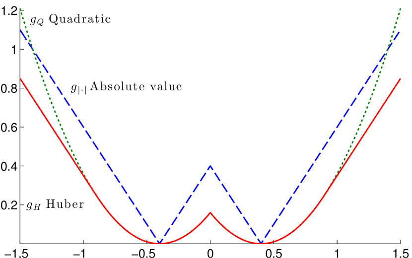
Fig. 1: The different cost functions considered in this paper: the maximum likelihood independent white gaussian noise $g_{Q}(x_{i},x_{j})=(\|x_{i}-x_{j}\|-d_{ij})^{2}$ shows the steepest tails, which act as outlier amplifiers; the $L_{1}$ loss $g_{|\cdot|}(x_{i},x_{j})=|\|x_{i}-x_{j}\|-d_{ij}|$, associated with impulsive noise, which fails to model the gaussianity of regular operating noise; and, finally, the Huber loss $g_{H}(x_{i},x_{j})=h_{R}(\|x_{i}-x_{j}\|-d_{ij})$, combines robustness to high-power outliers and adaptation to medium-power gaussian noise.

Figure 1 depicts a one-dimensional example of these different costs. We can observe in this simple example the main properties of the different cost functions, in terms of adaptation to low/medium-power gaussian noise and high-power outlier spikes. Using (1) we can write our optimization problem as

$$\operatornamewithlimits{minimize}_{x}g_{R}(x)$$ (2)

where

$$g_{R}(x)= \sum_{i\sim j}h_{R_{ij}}(\|x_{i}-x_{j}\|-d_{ij})+$$

$$\sum_{i}\sum_{k\in\mathcal{A}_{i}}h_{R_{ik}}(\|x_{i}-a_{k}\|-r_{ik}).$$ (3)

This function is nonconvex and, in general, difficult to minimize. We shall provide a convex underestimator, that tightly bounds each term of (3), thus leading to better estimation results than other relaxations which are not tight [8].

4 Convex underestimator

To convexify $g_{R}$ we can replace each term by its convex hull,

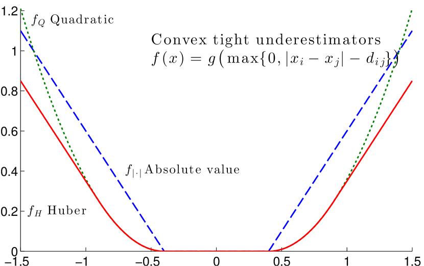
Fig. 2: All functions $f$ are tight underestimators to the functions $g$ in Figure 1. They are the convex envelopes and, thus, the best convex approximations to the original nonconvex costs. The convexification is performed by restricting the arguments of $g$ to be nonnegative.

as depicted in Figure 2. Here, we observe that the high-power behavior is maintained, whereas the medium/low-power is only altered in the convexified area. We define the convex costs by composition of any of the convex functions $h$ with a nondecreasing function $s$

$$s(t)=\max\{0,t\}$$

which, in turn, transforms the discrepancies

$$\delta_{ij}(x)=\|x_{i}-x_{j}\|-d_{ik},\qquad\delta_{ik}(x_{i})=\|x_{i}-a_{k}\|-r_{ik}.$$

As $s\left(\delta_{ij}(x)\right)$ and $s\left(\delta_{ik}(x)\right)$ are nondecreasing and each one of the functions $h$ is convex, then

$$f(x)= \sum_{i\sim j}h\left(s\left(\|x_{i}-x_{j}\|-d_{ij}\right)\right)+$$

$$\sum_{i}\sum_{k\in\mathcal{A}_{i}}h\left(s\left(\|x_{i}-a_{k}\|-r_{ik}\right)\right)$$

is also convex. The quality of the convexified quadratic problem was addressed in [10] and the analysis for the remaining functions is similar.

5 Numerical experiments

We assess the performance of the three considered loss functions through simulation. The experimental setup consists in a uniquely localizable geometric network deployed in a square area with side of $1$Km, with four anchors (blue squares in Figure 3) located at the corners, and ten sensors, (red stars). Measurements are also visible as dotted green lines. The average node degree of the network is $4.3$. The regular noisy range measurements are generated according to

$$d_{ij} = |\|x_{i}^{\star}-x_{j}^{\star}\|+\nu_{ij}|,\;r_{ik} = |\|x_{i}^{\star}-a_{k}\|+\nu_{ik}|,$$ (4)

where $x_{i}^{\star}$ is the true position of node $i$, and $\{\nu_{ij}:i\sim j\in\mathcal{E}\}\cup\{\nu_{ik}:i\in\mathcal{V},k\in\mathcal{A}_{i}\}$ are independent gaussian random variables with zero mean and standard deviation $0.04$, corresponding to an uncertainty of about $40$m. Node $7$ is malfunctioning and all measurements related to it are perturbed with gaussian noise with standard deviation $4$, corresponding to an uncertainty of $4$Km. The convex optimization problems were solved with cvx [11]. We ran $100$ Monte Carlo trials, sampling both regular and outlier noise.

The performance metric used to assess accuracy is the average positioning error defined as

$$\epsilon=\frac{1}{MC}\sum_{mc=1}^{MC}\|\hat{x}(mc)-x^{\star}\|.$$ (5)

where $MC$ is the number of Monte Carlo trials performed and $\hat{x}(mc)$ corresponds to the full set of estimates at trial $mc$.

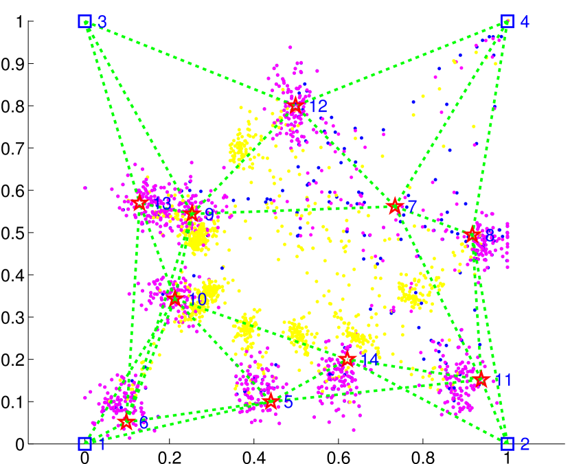
Fig. 3: Estimates for sensor positions for the three loss functions; We plotted in yellow the monte carlo results of minimizing $g_{|\cdot|}$, the $L_{1}$ loss; in blue we can see the estimates resulting from minimizing $g_{Q}$; in the same way, magenta dots represent the output for function $g_{R}$. It is noticeable that the $L_{1}$ loss is not able to correctly estimate positions whose measurements are corrupted with gaussian noise. The perturbation in node $7$ has more impact in the augmented dispersion of blue dots than magenta dots around its neighbors.

In Figure 3 we can observe that clouds of estimates from $g_{R}$ and $g_{Q}$ gather around the true positions, except for the malfunctioning node $7$. Note the spread of blue dots in the surroundings of the edges connecting node $7$, indicating that $g_{R}$ better preserves the nodes’ ability to localize themselves, despite their confusing neighbor $7$.

Table 1: Average positioning error per sensor ($\epsilon$/sensor), in meters

$f_{|\cdot|}$	$f_{Q}$	$f_{R}$
59.50	32.16	31.06

This intuition is confirmed by the analysis of the data in Table 1, which demonstrates that, even with only one disrupted sensor, our robust cost can reduce the error per sensor by $1.1$ meters. Also, as expected, the malfunctioning node cannot be positioned.

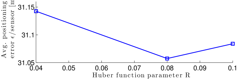
Fig. 4: Average positioning error versus the value of the Huber function parameter $R$. The accuracy is maintained even for different parameter values.

The sensitivity to the value of the Huber parameter $R$ in (1) is moderate, as shown in Figure 4. In fact, the error per sensor of the proposed estimator is always the smallest for all tested values of the parameter. We observe that the error increases when $R$ approaches the standard deviation of the regular gaussian noise, meaning that the Huber loss gets closer to the $L_{1}$ loss and, thus, is no longer adapted to the regular noise ($R=0$ corresponds exactly to the $L_{1}$ loss); in the same way, as $R$ increases, so does the quadratic section, and the estimator gets less robust to outliers, so, again, the error increases.

Another interesting experiment is to see what happens when the faulty sensor produces measurements with consistent errors or bias. So, we ran $100$ Monte Carlo trials in the same setting, but node $7$ measurements are consistently $10\%$ of the real distance to each neighbor.

Table 2: Average positioning error per sensor ($\epsilon$/sensor), in meters, for the biased experiment

$f_{|\cdot|}$	$f_{Q}$	$f_{R}$
80.98	58.31	47.08

The average positioning error per sensor is shown in Table 2. Here we observe a significant performance gap between the alternative costs, and our formulation proves to be, by far, superior.

6 Conclusions and future work

We proposed a dissimilarity model easy to motivate and effective, which accounts for outliers without prescribing a model for outlier noise. This dissimilarity model was convexified by means of the convex envelopes of its terms, leading to a problem with a unique minimum value attainable in polynomial time.

Different types of algorithms can be designed to attack the discrepancy measure presented in this work, since the function is continuous and convex. Due to the distributed nature of networks of sensors or, generically, agents, we aim at investigating a distributed minimization of the proposed robust loss. There are also several nice properties regarding distributed operation: the adjustable Huber parameter which is local to each edge and can be dynamically adjusted to the local environmental noise conditions, in a distributed manner.

Nevertheless, distributed implementation is a challenge, since the proposed loss lacks smoothness properties which were valuable in our previous work [10].

References

- [1] A.T. Ihler, J.W. Fisher III, R.L. Moses, and A.S. Willsky, “Nonparametric belief propagation for self-localization of sensor networks,” Selected Areas in Communications, IEEE Journal on, vol. 23, no. 4, pp. 809 – 819, April 2005.
- [2] J.N. Ash and R.L. Moses, “Outlier compensation in sensor network self-localization via the EM algorithm,” in Acoustics, Speech, and Signal Processing, 2005. Proceedings. (ICASSP ’05). IEEE International Conference on, March 2005, vol. 4, pp. iv/749–iv/752 Vol. 4.
- [3] Feng Yin, AM. Zoubir, C. Fritsche, and F. Gustafsson, “Robust cooperative sensor network localization via the EM criterion in LOS/NLOS environments,” in Signal Processing Advances in Wireless Communications (SPAWC), 2013 IEEE 14th Workshop on, June 2013, pp. 505–509.
- [4] P. Oguz-Ekim, J.P. Gomes, J. Xavier, and P. Oliveira, “Robust localization of nodes and time-recursive tracking in sensor networks using noisy range measurements,” Signal Processing, IEEE Transactions on, vol. 59, no. 8, pp. 3930 –3942, aug. 2011.
- [5] P.A. Forero and G.B. Giannakis, “Sparsity-exploiting robust multidimensional scaling,” Signal Processing, IEEE Transactions on, vol. 60, no. 8, pp. 4118 –4134, Aug. 2012.
- [6] S. Korkmaz and A-J. van der Veen, “Robust localization in sensor networks with iterative majorization techniques,” in Acoustics, Speech and Signal Processing, 2009. ICASSP 2009. IEEE International Conference on, April 2009, pp. 2049–2052.
- [7] Peter J. Huber, “Robust estimation of a location parameter,” The Annals of Mathematical Statistics, vol. 35, no. 1, pp. 73–101, 1964.
- [8] A. Simonetto and G. Leus, “Distributed maximum likelihood sensor network localization,” Signal Processing, IEEE Transactions on, vol. 62, no. 6, pp. 1424–1437, March 2014.
- [9] Jean-Baptiste Hiriart-Urruty and Claude Lemaréchal, Convex analysis and minimization algorithms, Springer-Verlag Limited, 1993.
- [10] Cláudia Soares, João Xavier, and João Gomes, “Simple and fast cooperative localization for sensor networks,” arXiv preprint arXiv:1408.4728, 2014.
- [11] Michael Grant and Stephen Boyd, “CVX: Matlab software for disciplined convex programming, version 2.1,” http://cvxr.com/cvx, Mar. 2014.