Principal Component Analysis for Second-order Stationary Vector Time Series

Abstract

We extend the principal component analysis (PCA) to second-order stationary vector time series in the sense that we seek for a contemporaneous linear transformation for a $p$-variate time series such that the transformed series is segmented into several lower-dimensional subseries, and those subseries are uncorrelated with each other both contemporaneously and serially. Therefore those lower-dimensional series can be analysed separately as far as the linear dynamic structure is concerned. Technically it boils down to an eigenanalysis for a positive definite matrix. When $p$ is large, an additional step is required to perform a permutation in terms of either maximum cross-correlations or FDR based on multiple tests. The asymptotic theory is established for both fixed $p$ and diverging $p$ when the sample size $n$ tends to infinity. Numerical experiments with both simulated and real data sets indicate that the proposed method is an effective initial step in analysing multiple time series data, which leads to substantial dimension reduction in modelling and forecasting high-dimensional linear dynamical structures. Unlike PCA for independent data, there is no guarantee that the required linear transformation exists. When it does not, the proposed method provides an approximate segmentation which leads to the advantages in, for example, forecasting for future values. The method can also be adapted to segment multiple volatility processes.

, and

t1Supported in part by the Fundamental Research Funds for the Central Universities (Grant No. JBK150501), NSFC (Grant No. 11501462), the Center of Statistical Research at SWUFE, and the Joint Lab of Data Science and Business Intelligence at SWUFE. t2Supported in part by the Fundamental Research Funds for the Central Universities (Grant No. JBK120509, JBK140507) and the Center of Statistical Research at SWUFE. t3Supported in part by an EPSRC research grant.

1 Introduction

Modelling multiple time series, also called vector time series, is always a challenge, even when the vector dimension $p$ is moderately large. While most the inference methods and the associated theory for univariate autoregressive and moving average (ARMA) processes have found their multivariate counterparts (Lütkepohl, 2006), vector autoregressive and moving average (VARMA) models are seldom used directly in practice when $p\geq 3$. This is partially due to the lack of identifiability for VARMA models in general. More fundamentally, those models are overparametrized; leading to flat likelihood functions which cause innate difficulties in statistical inference. Therefore finding an effective way to reduce the number of parameters is particularly felicitous in modelling and forecasting multiple time series. The urge for doing so is more pertinent in this modern information age, as it has become commonplace to access and to analyse high dimensional time series data with dimension $p$ in the order of hundreds or more. Big time series data arise from, among others, panel study for economic and natural phenomena, social network, healthcare and public health, financial market, supermarket transactions, information retrieval and recommender systems.

Available methods to reduce the number of parameters in modelling vector time series can be divided into two categories: regularization and dimension reduction. The former imposes some conditions on the structure of a VARMA model. The latter represents a high-dimensional process in terms of several lower-dimensional processes. Various regularization methods have been developed in literature. For example, Jakeman, Steele and Young (1980) adopted a two stage regression strategy based on instrumental variables to avoid using moving average explicitly. Different canonical structures are imposed on VARMA models [Chapter 3 of Reinsel (1993), Chapter 4 of Tsay (2014), and references within]. Structural restrictions are imposed in order to specify and to estimate some reduced forms of vector autoregressive (VAR) models [Chapter 9 of Lütkepohl (2006), and references within]. Davis, Zang and Zheng (2012) proposed a VAR model with sparse coefficient matrices based on partial spectral coherence. Under different sparsity assumptions, VAR models have been estimated by LASSO regularization (Shojaie and Michailidis, 2010; Song and Bickel, 2011), or by the Dantzig selector (Han and Liu, 2013). Guo, Wang and Yao (2016) considered high-dimensional autoregression with banded coefficient matrices. The dimension reduction methods include the canonical correlation analysis of Box and Tiao (1977), the independent components analysis (ICA) of Back and Weigend (1997), the principal components analysis (PCA) of Stock and Watson (2002), the scalar component analysis of Tiao and Tsay (1989) and Huang and Tsay (2014), the dynamic orthogonal components analysis of Matteson and Tsay (2011). Another popular approach is to represent multiple time series in terms of a few latent factors defined in various ways. There is a large body of literature in this area published in the outlets in statistics, econometrics and signal processing. An incomplete list of the publications includes Anderson (1963), Peña and Box (1987), Tong, Xu and Kailath (1994), Belouchrani et al. (1997), Bai and Ng (2002), Theis, Meyer-Baese and Lang (2004), Stock and Watson (2005), Forni et al. (2005), Pan and Yao (2008), Lam, Yao and Bathia (2011), Lam and Yao (2012) and Chang, Guo and Yao (2015).

A new dimension reduction method is proposed in this paper. We seek for a contemporaneous linear transformation such that the transformed series is segmented into several lower-dimensional subseries, and those subseries are uncorrelated with each other both contemporaneously and serially. Therefore they can be modelled or forecasted separately, as far as linear dependence is concerned. This reduces the number of parameters involved in depicting linear dynamic structure substantially. While the basic idea is not new, which has been explored with various methods including some aforementioned references, the method proposed in this paper (i.e. the new PCA for time series) is new, simple and effective. Technically the proposed method boils down to an eigenanalysis for a positive definite matrix which is a quadratic function of the cross correlation matrix function for the observed process. Hence it is easy to implement and the required computation can be carried out with, for example, an ordinary personal computer or laptop for the data with dimension $p$ in the order of thousands.

The method can be viewed as an extension of the standard PCA for multiple time series, therefore, is abbreviated as TS-PCA. However the segmented subseries are not guaranteed to exist as those subseries must not correlate with each other across all times. This is a marked difference from the standard PCA. The real data examples in Section 4 indicate that it is often reasonable to assume that the segmentation exists. Furthermore, when the assumption is invalid, the proposed method provides some approximate segmentations which ignore some weak though significant correlations, and those weak correlations are of little practical use for modelling and forecasting. Thus the proposed method can be used as an initial step in analysing multiple time series, which often transforms a multi-dimensional problem into several lower-dimensional problems. Furthermore the results obtained for the transformed subseries can be easily transformed back to the original multiple time series. Illustration with real data examples indicates clearly the advantages in post-sample forecasting from using the proposed TS-PCA. The R-package PCA4TS, available from CRAN project, implements the proposed methodology.

The proposed TS-PCA can be viewed as a version of ICA. In fact our goal is the same in principle as the ICA using autocovariances presented in Section 18.1 of Hyvärinen, Karhunen and Oja (2001). However, the nonlinear optimization algorithms presented there are to search for a linear transformation such that all the off-diagonal elements of the autocovariance matrices for the transformed vector time series are minimized. See also Tong, Xu and Kailath (1994), and Belouchrani et al. (1997). To apply those algorithms to our setting, we need to know exactly the block diagonal structure of autocovariances of the transformed vector process (i.e. the number of blocks and the sizes of all the blocks), which is unknown in practice. Furthermore, our method is simple and fast, and therefore is applicable to high-dimensional cases. Cardoso (1998) extends the basic idea of ICA to the so called multivariate ICA, which requires the transformed random vector to be segmented into several independent groups with possibly more than one component in each group. But Cardoso (1998) does not provide a pertinent algorithm for multivariate ICA. Furthermore it does not consider the dependence across different time lags. TS-PCA is also different from the dynamic PCA proposed in Chapter 9 of Brillinger (1981) which decomposes each component time series as the sum of moving averages of several uncorrelated white noise processes. In our TS-PCA, no lagged variables enter the decomposition.

The rest of the paper is organised as follows. The methodology is spelled out in Section 2. Section 3 presents the associated asymptotic properties of the proposed method. Numerical illustration with real data are reported in Section 4. Section 5 extends the method to segmenting a multiple volatility process into several lower-dimensional volatility processes. Some final remarks are given in Section 6. All technical proofs and numerical illustration with simulated data are relegated to the supplementary material [Chang, Guo and Yao (2016)]. We always use the following notation. For any $m\times k$ matrix ${\mathbf{H}}=(h_{i,j})$, let $\|{\mathbf{H}}\|_{2}=\lambda_{\max}^{1/2}({\mathbf{H}}{\mathbf{H}}^{\mathrm{\scriptscriptstyle T}})$ and $\|{\mathbf{H}}\|_{F}=(\sum_{i=1}^{m}\sum_{j=1}^{k}h_{i,j}^{2})^{1/2},$ where $\lambda_{\max}({\mathbf{H}}{\mathbf{H}}^{\mathrm{\scriptscriptstyle T}})$ denotes the largest eigenvalue of ${\mathbf{H}}{\mathbf{H}}^{\mathrm{\scriptscriptstyle T}}$.

2 Methodology

2.1 Setting and method

Let ${\mathbf{y}}_{t}$ be observable $p\times 1$ weakly stationary time series. We assume that ${\mathbf{y}}_{t}$ admits a latent segmentation structure:

$${\mathbf{y}}_{t}={\mathbf{A}}{\mathbf{x}}_{t},$$ (2.1)

where ${\mathbf{x}}_{t}$ is an unobservable $p\times 1$ weakly stationary time series consisting of $q\;(>1)$ both contemporaneously and serially uncorrelated subseries, and ${\mathbf{A}}$ is an unknown constant matrix. Hence all the autocovariances of ${\mathbf{x}}_{t}$ are of the same block-diagonal structure with $q$ blocks. Denote the segmentation of ${\mathbf{x}}_{t}$ by

$${\mathbf{x}}_{t}=({\mathbf{x}}_{t}^{(1),{\mathrm{\scriptscriptstyle T}}},\ldots,{\mathbf{x}}_{t}^{(q),{\mathrm{\scriptscriptstyle T}}})^{{\mathrm{\scriptscriptstyle T}}}$$ (2.2)

with ${\rm Cov}({\mathbf{x}}_{t}^{(i)},{\mathbf{x}}_{s}^{(j)})={\bf 0}$ for all $t,s$ and $i\neq j$. Therefore ${\mathbf{x}}_{t}^{(1)},\ldots,{\mathbf{x}}_{t}^{(q)}$ can be modelled or forecasted separately as far as their linear dynamic structure is concerned.

Example 1.

Before we spell out how to find the segmentation transformation ${\mathbf{A}}$ in general, we consider the monthly temperatures of 7 cities (Nanjing, Dongtai, Huoshan, Hefei, Shanghai, Anqing and Hangzhou) in Eastern China from January 1954 to December 1998. Fig 1(a) plots the cross correlations of these 7 temperature time series. Both the autocorrelation of each component series and the cross correlation between any two component series are dominated by the annual temperature fluctuation; showing the strong periodicity with the period 12. Now we apply the linear transformation ${\mathbf{x}}_{t}={\mathbf{A}}^{-1}{\mathbf{y}}_{t}$ with

$${\mathbf{A}}^{-1}=\left(\begin{array}[]{rrrrrrr}0.244&-0.066&0.019&-0.050&-0.313&-0.154&0.200\\ -0.703&0.324&-0.617&0.189&0.633&0.499&-0.323\\ 0.375&1.544&-1.615&0.170&-2.266&0.126&1.596\\ 3.025&-1.381&-0.787&-1.691&-0.212&1.188&-0.165\\ -0.197&-1.820&-1.416&3.269&0.301&-1.438&1.299\\ -0.584&-0.354&0.847&-1.262&-0.218&-0.151&1.831\\ 1.869&-0.742&0.034&0.501&0.492&-2.533&0.339\end{array}\right),$$

where ${\bf A}$ is determined by the method given in Section 2. Fig 1(b) shows that the first two transformed component series are significantly correlated both concurrently and serially, and there are also small but significant correlations in the (3, 2)-th panel; indicating the correlations between the 2nd and the 3rd component series. Apart from these, there is little significant cross correlation among all the other pairs of component series. This visual observation suggests to segment the 7 transformed series into 5 uncorrelated groups: {1, 2, 3}, {4}, {5}, {6} and {7}.

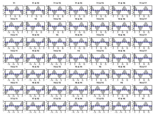
(a) Cross correlogram of the original $7$ temperature time series.

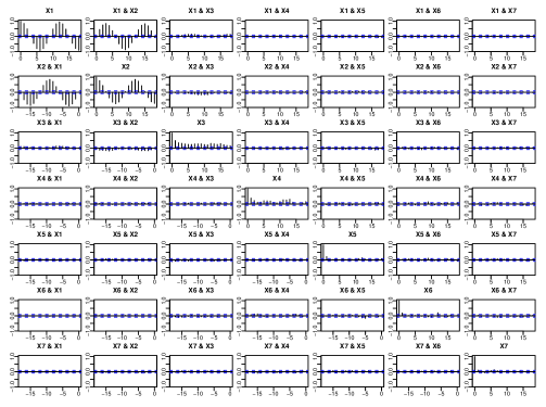
(b) Cross correlogram of the $7$ transformed component time series.

Figure 1: Cross correlograms for Example 1.

This example indicates that the segmentation transformation transfers the problem of analysing a 7-dimensional time series into the five lower-dimensional problems: four univariate time series and one 3-dimensional time series. Those five time series can and should be analysed separately as there are no cross correlations among them at all time lags. The linear dynamic structure of the original series is deduced by those of the five transformed series, as ${\rm Cov}({\mathbf{y}}_{t+k},{\mathbf{y}}_{t})={\mathbf{A}}{\rm Cov}({\mathbf{x}}_{t+k},{\mathbf{x}}_{t}){\mathbf{A}}^{\mathrm{\scriptscriptstyle T}}$.

Now we spell out how to find the segmentation transformation under (2.1) and (2.2). Without the loss of generality we may assume

$$\mbox{Var}({\mathbf{y}}_{t})={\mathbf{I}}_{p}~{}~{}{\rm and}~{}~{}\mbox{Var}({\mathbf{x}}_{t})={\mathbf{I}}_{p},$$ (2.3)

where ${\mathbf{I}}_{p}$ denotes the $p\times p$ identity matrix. This first equation in (2.3) amounts to replace ${\mathbf{y}}_{t}$ by $\widehat{\mathbf{V}}^{-{1/2}}{\mathbf{y}}_{t}$ as a preliminary step in practice, where $\widehat{\mathbf{V}}$ is a consistent estimator for $\mbox{Var}({\mathbf{y}}_{t})$. As both ${\mathbf{A}}$ and ${\mathbf{x}}_{t}$ are unobservable, the second equation in (2.3) implies that we view $({\mathbf{A}}\{\mbox{Var}({\mathbf{x}}_{t})\}^{1/2},\linebreak\{\mbox{Var}({\mathbf{x}}_{t})\}^{-{1/2}}{\mathbf{x}}_{t})$ as $({\mathbf{A}},{\mathbf{x}}_{t})$ in (2.1). More importantly, the latter perspective will not alter the block-diagonal structure of the autocovariance matrices of ${\mathbf{x}}_{t}$. Now it follows from (2.1) and (2.3) that ${\mathbf{I}}_{p}=\mbox{Var}({\mathbf{y}}_{t})={\mathbf{A}}\mbox{Var}({\mathbf{x}}_{t}){\mathbf{A}}^{\mathrm{\scriptscriptstyle T}}={\mathbf{A}}{\mathbf{A}}^{\mathrm{\scriptscriptstyle T}}.$ Thus, ${\mathbf{A}}$ in (2.1) is an orthogonal matrix under (2.3).

Let $p_{j}$ be the length of ${\mathbf{x}}_{t}^{(j)}$. Write ${\mathbf{A}}=({\mathbf{A}}_{1},\ldots,{\mathbf{A}}_{q})$, where ${\mathbf{A}}_{j}$ has $p_{j}$ columns. Since ${\mathbf{x}}_{t}={\mathbf{A}}^{\mathrm{\scriptscriptstyle T}}{\mathbf{y}}_{t}$, it follows from (2.2) that

$${\mathbf{x}}_{t}^{(j)}={\mathbf{A}}_{j}^{\mathrm{\scriptscriptstyle T}}{\mathbf{y}}_{t},\quad j=1,\ldots,q.$$ (2.4)

Let ${\mathbf{H}}_{j}$ be any $p_{j}\times p_{j}$ orthogonal matrix, and ${\mathbf{H}}={\rm diag}({\mathbf{H}}_{1},\ldots,{\mathbf{H}}_{q})$. Then $({\mathbf{A}},\,{\mathbf{x}}_{t})$ in (2.1) can be replaced by $({\mathbf{A}}{\mathbf{H}},\,{\mathbf{H}}^{\mathrm{\scriptscriptstyle T}}{\mathbf{x}}_{t})$ while (2.2) still holds. Hence ${\mathbf{A}}$ and ${\mathbf{x}}_{t}$ are not uniquely identified in (2.1), even with the additional assumption (2.3). In fact under (2.3), only $\mathcal{M}({\mathbf{A}}_{1}),\ldots,\mathcal{M}({\mathbf{A}}_{q})$ are uniquely defined by (2.1), where $\mathcal{M}({\mathbf{A}}_{j})$ denotes the linear space spanned by the columns of ${\mathbf{A}}_{j}$. Consequently, $\boldsymbol{\Gamma}_{j}^{\mathrm{\scriptscriptstyle T}}{\mathbf{y}}_{t}$ can be taken as ${\mathbf{x}}_{t}^{(j)}$ for any $p\times p_{j}$ matrix $\boldsymbol{\Gamma}_{j}$ as long as $\boldsymbol{\Gamma}_{j}^{\mathrm{\scriptscriptstyle T}}\boldsymbol{\Gamma}_{j}={\mathbf{I}}_{p_{j}}$ and $\mathcal{M}(\boldsymbol{\Gamma}_{j})=\mathcal{M}({\mathbf{A}}_{j})$.

To discover the latent segmentation, we need to estimate ${\mathbf{A}}=({\mathbf{A}}_{1},\ldots,{\mathbf{A}}_{q})$, or more precisely, to estimate linear spaces $\mathcal{M}({\mathbf{A}}_{1}),\ldots,\mathcal{M}({\mathbf{A}}_{q})$. To this end, we introduce some notation first. For any integer $k$, let $\boldsymbol{\Sigma}_{y}(k)={\rm Cov}({\mathbf{y}}_{t+k},{\mathbf{y}}_{t})$ and $\boldsymbol{\Sigma}_{x}(k)={\rm Cov}({\mathbf{x}}_{t+k},{\mathbf{x}}_{t}).$ For a prescribed positive integer $k_{0}$, define

$${\mathbf{W}}_{y} =\sum_{k=0}^{k_{0}}\boldsymbol{\Sigma}_{y}(k)\boldsymbol{\Sigma}_{y}(k)^{\mathrm{\scriptscriptstyle T}}={\mathbf{I}}_{p}+\sum_{k=1}^{k_{0}}\boldsymbol{\Sigma}_{y}(k)\boldsymbol{\Sigma}_{y}(k)^{\mathrm{\scriptscriptstyle T}},$$ (2.5)

$${\mathbf{W}}_{x} =\sum_{k=0}^{k_{0}}\boldsymbol{\Sigma}_{x}(k)\boldsymbol{\Sigma}_{x}(k)^{\mathrm{\scriptscriptstyle T}}={\mathbf{I}}_{p}+\sum_{k=1}^{k_{0}}\boldsymbol{\Sigma}_{x}(k)\boldsymbol{\Sigma}_{x}(k)^{\mathrm{\scriptscriptstyle T}}.$$

Then both $\boldsymbol{\Sigma}_{x}(k)$ and ${\mathbf{W}}_{x}$ are block-diagonal, and

$${\mathbf{W}}_{y}={\mathbf{A}}{\mathbf{W}}_{x}{\mathbf{A}}^{\mathrm{\scriptscriptstyle T}}.$$ (2.6)

Note that both ${\mathbf{W}}_{y}$ and ${\mathbf{W}}_{x}$ are positive definite matrices. Let

$${\mathbf{W}}_{x}\boldsymbol{\Gamma}_{x}=\boldsymbol{\Gamma}_{x}{\mathbf{D}},$$ (2.7)

i.e. $\boldsymbol{\Gamma}_{x}$ is a $p\times p$ orthogonal matrix with the columns being the orthonormal eigenvectors of ${\mathbf{W}}_{x}$, and ${\mathbf{D}}$ is a diagonal matrix with the corresponding eigenvalues as the elements on the main diagonal. Then (2.6) implies that ${\mathbf{W}}_{y}{\mathbf{A}}\boldsymbol{\Gamma}_{x}={\mathbf{A}}\boldsymbol{\Gamma}_{x}{\mathbf{D}}.$ Hence the columns of $\boldsymbol{\Gamma}_{y}\equiv{\mathbf{A}}\boldsymbol{\Gamma}_{x}$ are the orthonormal eigenvectors of ${\mathbf{W}}_{y}$. Consequently,

$$\boldsymbol{\Gamma}_{y}^{\mathrm{\scriptscriptstyle T}}{\mathbf{y}}_{t}=\boldsymbol{\Gamma}_{x}^{\mathrm{\scriptscriptstyle T}}{\mathbf{A}}^{\mathrm{\scriptscriptstyle T}}{\mathbf{y}}_{t}=\boldsymbol{\Gamma}_{x}^{\mathrm{\scriptscriptstyle T}}{\mathbf{x}}_{t},$$ (2.8)

the last equality follows from (2.1). Put

$${\mathbf{W}}_{x}={\rm diag}({\mathbf{W}}_{x,1},\ldots,{\mathbf{W}}_{x,q}).$$ (2.9)

Then ${\mathbf{W}}_{x,j}$ is a $p_{j}\times p_{j}$ positive definite matrix, and the eigenvalues of ${\mathbf{W}}_{x,j}$ are also the eigenvalues of ${\mathbf{W}}_{x}$. Suppose that ${\mathbf{W}}_{x,i}$ and ${\mathbf{W}}_{x,j}$ do not share the same eigenvalues for any $i\neq j$. Then if we line up the eigenvalues of ${\mathbf{W}}_{x}$ (i.e. the eigenvalues of ${\mathbf{W}}_{x,1},\ldots,{\mathbf{W}}_{x,q}$ combining together) in the main diagonal of ${\mathbf{D}}$ according to the order of the blocks in ${\mathbf{W}}_{x}$, $\boldsymbol{\Gamma}_{x}$ must be a block-diagonal orthogonal matrix of the same shape as ${\mathbf{W}}_{x}$; see Proposition 1(i). However the order of the eigenvalues is latent, and any $\boldsymbol{\Gamma}_{x}$ defined by (2.7) is nevertheless a column-permutation of such a block-diagonal orthogonal matrix; see Proposition 1(ii). Hence each component of $\boldsymbol{\Gamma}_{x}^{\mathrm{\scriptscriptstyle T}}{\mathbf{x}}_{t}$ is a linear transformation of the elements in one of the $q$ subseries only, i.e. the $p$ components of $\boldsymbol{\Gamma}_{y}^{\mathrm{\scriptscriptstyle T}}{\mathbf{y}}_{t}=\boldsymbol{\Gamma}_{x}^{\mathrm{\scriptscriptstyle T}}{\mathbf{x}}_{t}$ can be partitioned into the $q$ groups such that there exist neither contemporaneous nor serial correlations across different groups. Thus $\boldsymbol{\Gamma}_{y}^{\mathrm{\scriptscriptstyle T}}{\mathbf{y}}_{t}$ can be regarded as a permutation of ${\mathbf{x}}_{t}$, and $\boldsymbol{\Gamma}_{y}$ can be viewed as a column-permutation of ${\mathbf{A}}$; see the discussion below (2.4). This leads to the following two-step estimation for ${\mathbf{A}}$ and ${\mathbf{x}}_{t}$:

Step 1.

Let $\widehat{\mathbf{S}}$ be an estimator for ${\mathbf{W}}_{y}$. Calculate a $p\times p$ orthogonal matrix $\widehat{\boldsymbol{\Gamma}}_{y}$ with the columns being the orthonormal eigenvectors of $\widehat{\mathbf{S}}$.

Step 2.

The columns of $\widehat{\mathbf{A}}=(\widehat{\mathbf{A}}_{1},\ldots,\widehat{\mathbf{A}}_{q})$ are a permutation of the columns of $\widehat{\boldsymbol{\Gamma}}_{y}$ such that $\widehat{\mathbf{x}}_{t}=\widehat{\mathbf{A}}^{\mathrm{\scriptscriptstyle T}}{\mathbf{y}}_{t}$ is segmented into $q$ uncorrelated subseries $\widehat{\mathbf{x}}_{t}^{(j)}=\widehat{\mathbf{A}}_{j}^{\mathrm{\scriptscriptstyle T}}{\mathbf{y}}_{t}$, $j=1,\ldots,q$.

Step 1 is the key, as it provides an estimator for ${\mathbf{A}}$ except that the columns of the estimator are not grouped together according to the latent segmentation. The estimator $\widehat{\mathbf{S}}$ will be discussed in Section 3. The permutation in Step 2 above can be carried out in principle by visual observation: plot cross correlogram of $\widehat{\mathbf{z}}_{t}\equiv\widehat{\boldsymbol{\Gamma}}^{\mathrm{\scriptscriptstyle T}}_{y}{\mathbf{y}}_{t}$ (using, for example, R-function acf); see Fig 1(b). We then put those components of $\widehat{\mathbf{z}}_{t}$ together when there exist significant cross-correlations (at any lags) between those component series. Then $\widehat{\mathbf{A}}$ is obtained by re-arranging the order of the columns of $\widehat{\boldsymbol{\Gamma}}_{y}$ accordingly.

Remark 1.

(i) Appropriate precaution should be exercised in the visual observation stated above. First the visual observation become impractical when $p$ is large. Furthermore most correlogram plots produced by statistical packages (including R) use the confidence bounds at $\pm 1.96/\sqrt{n}$ for sample cross-correlations of two time series. Unfortunately those bounds are only valid if at least one of the two series is white noise. In general, the confidence bounds depend on the autocorrelations of the two series. See Theorem 7.3.1 of Brockwell and Davis (1996). In Section 2.2, we will describe how the permutation can be performed without the benefit of visual observation for the cross correlogram of $\widehat{\mathbf{z}}_{t}$. Ledoit and Wolf (2004) and Paparoditis and Politis (2012) provide more modern approaches to view correlations.

(ii) ${\mathbf{W}}_{y}$ defined in (2.5) combines the information over different time lags together. In practice we need to specify the integer $k_{0}$. Note that all terms on the right-hand side of (2.5) is non-negative definite. Hence there is no information cancellation over different lags. This makes the method insensitive to the choice of $k_{0}$. In practice a small $k_{0}$ is often sufficient, as long as the first $k_{0}$ lags carry sufficient information on the latent block diagonal structure even when the auto/cross-correlations beyond lag $k_{0}$ are still significant. The examples in Section 4 lend further support to this assertion.

Proposition 1.

(i) The orthogonal matrix $\boldsymbol{\Gamma}_{x}$ in (2.7) can be taken as a block-diagonal orthogonal matrix with the same block structure as ${\mathbf{W}}_{x}$.

(ii) An orthogonal matrix $\boldsymbol{\Gamma}_{x}$ satisfies (2.7) if and only if its columns are a permutation of the columns of a block-diagonal orthogonal matrix described in (i), provided that any two different blocks ${\mathbf{W}}_{x,i}$ and ${\mathbf{W}}_{x,j}$ do not share the same eigenvalues.

Proposition 1(ii) requires that the $q$ blocks of ${\mathbf{W}}_{x}$ do not share the same eigenvalue(s). However it does not rule out the possibility that each block ${\mathbf{W}}_{x,j}$ may have multiple eigenvalues. When different blocks share the same eigenvalue(s), Proposition 1 still holds with ${\mathbf{W}}_{x}$ replaced by ${\mathbf{W}}_{x}^{\star}$ which is also a block diagonal matrix with fewer than $q$ blocks obtained by combining together those ${\mathbf{W}}_{x,j}$’s sharing at least one common eigenvalue into one larger block. This means that the proposed method will not be able to separate, for example, ${\mathbf{x}}_{t}^{(1)}$ and ${\mathbf{x}}_{t}^{(2)}$ if ${\mathbf{W}}_{x,1}$ and ${\mathbf{W}}_{x,2}$ share at least one common eigenvalue.

2.2 Permutation

2.2.1 Permutation rule

The columns of $\widehat{\mathbf{A}}$ is a permutation of the columns of $\widehat{\boldsymbol{\Gamma}}_{y}$. The permutation is determined by grouping the components of $\widehat{\mathbf{z}}_{t}=\widehat{\boldsymbol{\Gamma}}_{y}^{\mathrm{\scriptscriptstyle T}}{\mathbf{y}}_{t}$ into $q$ groups, where $q$ and the cardinal numbers of those groups are unknown. Write $\widehat{\mathbf{z}}_{t}=(\widehat{z}_{1,t},\ldots,\widehat{z}_{p,t})^{\mathrm{\scriptscriptstyle T}}$. Let $\rho_{i,j}(h)$ denote the cross correlation between the two component series $\widehat{z}_{i,t}$ and $\widehat{z}_{j,t}$ at lag $h$. We say $\widehat{z}_{i,t}$ and $\widehat{z}_{j,t}$ connected if the multiple null hypothesis

$$H_{0}:\rho_{i,j}(h)=0\quad\mbox{for any $h=0,\pm 1,\pm 2,\ldots,\pm m$}$$ (2.10)

is rejected, where $m\geq 1$ is a prescribed integer. Thus there exists significant evidence indicating non-zero correlations between two connected component series. Hence those components should be put in the same group. We may take $m=20$, or $m$ sufficiently large but smaller than $n/4$, in the spirit of the rule of thumb proposed by Box and Jenkins (1970, p.30), as we exclude long memory processes in this paper. Note that the autocorrelations of stationary (causal) VARMA processes decay exponentially fast. The permutation in Step 2 in Section 2.1 can be performed as follows.

1. Start with the $p$ groups with each group containing one component of $\widehat{\mathbf{z}}_{t}$ only.

2. Combine two groups together if one connected pair are split over the two groups.

3. Repeat Step ii above until all connected pairs are within one group.

We introduce below two methods for identifying the connected pair components of $\widehat{\mathbf{z}}_{t}=\widehat{\boldsymbol{\Gamma}}_{y}^{\mathrm{\scriptscriptstyle T}}{\mathbf{y}}_{t}$.

2.2.2 Maximum cross correlation method

One natural way to test hypothesis $H_{0}$ in (2.10) is to use the maximum cross correlation over the lags between $-m$ and $m$:

$$\widehat{L}_{n}(i,j)=\max_{|h|\leq m}|\widehat{\rho}_{i,j}(h)|,$$ (2.11)

where $\widehat{\rho}_{i,j}(h)$ is the sample cross correlation between $\widehat{z}_{i,t}$ and $\widehat{z}_{j,t}$ at lag $h$. We would reject $H_{0}$ for the pair $(\widehat{z}_{i,t},\widehat{z}_{j,t})$ if $\widehat{L}_{n}(i,j)$ is greater than an appropriate threshold value.

Instead of conducting multiple tests for each of the $p_{0}\equiv p(p-1)/2$ pairs components of $\widehat{\mathbf{z}}_{t}$, we propose a ratio-based statistic to single out those pairs for which $H_{0}$ will be rejected. To this end, we re-arrange the $p_{0}$ obtained $\widehat{L}_{n}(i,j)$’s in the descending order: $\widehat{L}_{1}\geq\cdots\geq\widehat{L}_{p_{0}}$. Define

$$\widehat{r}=\arg\max_{1\leq j<c_{0}p_{0}}\widehat{L}_{j}/\widehat{L}_{j+1},$$ (2.12)

where $c_{0}\in(0,1)$ is a prescribed constant. In all the numerical examples in Section 4 and the supplementary material [Chang, Guo and Yao (2016)] we use $c_{0}=0.75$. We reject $H_{0}$ for the pairs corresponding to $\widehat{L}_{1},\ldots,\widehat{L}_{\widehat{r}}$.

The intuition behind this approach is as follows. Suppose among in total $p_{0}$ pairs of the components of ${\mathbf{x}}_{t}$ there are $r$ connected pairs only. Arrange the true maximum cross correlations in the descending order: $L_{1}\geq\cdots\geq L_{p_{0}}$. Then $L_{r}>0$ and $L_{r+1}=0$, and the ratio $L_{j}/L_{j+1}$ takes value $\infty$ for $j=r$. This motivates the estimator $\widehat{r}$ defined in (2.12) in which we exclude some minimum $\widehat{L}_{j}$ in the search for $\widehat{r}$ as $c_{0}\in(0,1)$. This is to avoid the fluctuations due to the ratios of extreme small values. This causes little loss in information as, for example, $0.75p_{0}$ connected pairs would likely group most, if not all, component series together; see, e.g., Example 3 in Section 4. The similar idea has been used in defining the factor dimensions in Lam and Yao (2012) and Chang, Guo and Yao (2015).

To state the asymptotic property of the above approach, we use a graph representation. Let the graph contain $p$ vertexes $\widehat{V}=\{1,\ldots,p\}$, representing $p$ component series of $\widehat{\mathbf{z}}_{t}$. Define an edge connecting vertexes $i$ and $j$ if $H_{0}$ in (2.10) for $(\widehat{z}_{i,t},\widehat{z}_{j,t})$ is rejected by the above ratio method. Let $\widehat{E}_{n}$ be the set consisting all those edges. Let $V=\{1,\ldots,p\}$ represent the $p$ component series of ${\mathbf{z}}_{t}=\boldsymbol{\Gamma}_{y}^{\mathrm{\scriptscriptstyle T}}{\mathbf{y}}_{t}$ defined in (2.8), and write ${\mathbf{z}}_{t}=(z_{1,t},\ldots,z_{p,t})^{\mathrm{\scriptscriptstyle T}}$. Define

$$E=\Big{\{}(i,j):\max_{|h|\leq m}|{\rm Corr}(z_{i,t+h},z_{j,t})|>0,\,1\leq i<j\leq p\Big{\}}.$$

Each $(i,j)\in E$ can be reviewed as an edge. The graph $(\widehat{V},\widehat{E}_{n})$ is a consistent estimate for the graph $(V,E)$; see Proposition 2 below. To avoid the technical difficulties in dealing with ‘0/0’, we modify (2.12) as follows:

$$\widehat{r}=\arg\max_{1\leq j<p_{0}}(\widehat{L}_{j}+\delta_{n})/(\widehat{L}_{j+1}+\delta_{n}),$$ (2.13)

where $\delta_{n}>0$ is a small constant. Assume

$$\min_{(i,j)\in E}\max_{|h|\leq m}|{\rm Corr}(z_{i,t+h},z_{j,t})|\geq\epsilon_{n}$$

for some $\epsilon_{n}>0$ and $n\epsilon_{n}^{2}\rightarrow\infty$. Write

$$\varpi_{n}=\min_{1\leq i<j\leq p}\min_{\lambda\in\sigma({\mathbf{W}}_{x,i}),\mu\in\sigma({\mathbf{W}}_{x,j})}|\lambda-\mu|,$$ (2.14)

where ${\mathbf{W}}_{x,i}$ is defined in (2.9), $\sigma({\mathbf{W}}_{x,i})$ denotes the set consisting of all the eigenvalues of ${\mathbf{W}}_{x,i}$. Here $\epsilon_{n}$ denotes the weakest signal to be identified in $E$, and $\varpi_{n}$ is the minimum difference between the eigenvalues from the different diagonal blocks in ${\mathbf{W}}_{x}$. Arrange the true maximum cross correlations of ${\mathbf{z}}_{t}$ in the descending order $L_{1}\geq\cdots\geq L_{p_{0}}$ and define

$$\chi_{n}=\max_{1\leq j<r-1}L_{j}/L_{j+1},$$

where $r=|E|$. Recall that $\widehat{\mathbf{S}}$ is the estimator for ${\mathbf{W}}_{y}$ used in Step 1 in Section 2.1. Let

$$\widehat{\boldsymbol{\Sigma}}_{y}(h)={1\over n}\sum_{t=1}^{n-h}({\mathbf{y}}_{t+h}-\bar{\mathbf{y}})({\mathbf{y}}_{t}-\bar{\mathbf{y}})^{\mathrm{\scriptscriptstyle T}}~{}~{}{\rm and}~{}~{}\bar{\mathbf{y}}={1\over n}\sum_{t=1}^{n}{\mathbf{y}}_{t}.$$ (2.15)

Now we state the consistency in Proposition 2, which requires $\varpi_{n}>0$ [see Proposition 1(ii)]. The proof of Proposition 2 is similar to that of Theorem 2.4 of Chang, Guo and Yao (2015), and is therefore omitted.

Proposition 2.

Let $\chi_{n}\delta_{n}=o(\epsilon_{n})$ and $\varpi_{n}^{-1}\|\widehat{{\mathbf{S}}}-{\mathbf{W}}_{y}\|_{2}=o_{p}(\delta_{n})$. Let the singular values of $\widehat{\boldsymbol{\Sigma}}_{y}(h)$ be uniformly bounded away from $\infty$ for all $|h|\leq m$. Then for $\widehat{r}$ defined in (2.13), it holds that $\mathbb{P}(\widehat{E}_{n}=E)\to 1$.

Remark 2.

(i) The inserting of $\delta_{n}$ in the definition of $\widehat{r}$ in (2.13) is to avoid the undetermined “0/0” cases. In practice, we use $\widehat{r}$ defined by (2.12) instead, but with the search restricted to $1\leq j\leq c_{0}p_{0}$, as $\delta_{n}$ subscribed in Proposition 2 is unknown. The simulation results reported in the supplementary material [Chang, Guo and Yao (2016)] indicate that (2.12) works reasonably well. See also Lam and Yao (2012) and Chang, Guo and Yao (2015).

(ii) The uniform boundedness for the singular values of $\widehat{\boldsymbol{\Sigma}}_{y}(h)$ was used to simplify the presentation. If $\max_{|h|\leq m}\|\widehat{\boldsymbol{\Sigma}}_{y}(h)\|_{2}=O_{p}(\nu_{n})$ for some diverging $\nu_{n}$, we require the condition $\varpi_{n}^{-1}\nu_{n}\|\widehat{{\mathbf{S}}}-{\mathbf{W}}_{y}\|_{2}=o_{p}(\delta_{n})$.

(iii) The finite sample performance can be improved by prewhitening each component series $\widehat{z}_{i,t}$ first. Then the asymptotic variance of $\widehat{\rho}_{i,j}(h)$ is $1/n$ as long as ${\rm Corr}(z_{i,t+h},z_{j,t})=0$, see Corollary 7.3.1 of Brockwell and Davis (1996). This makes the maximum cross correlations for different pairs more comparable. Note that two weakly stationary time series are correlated if and only if their prewhitened series are correlated.

2.2.3 FDR based on multiple tests

Alternatively we can identify the connected pair components of $\widehat{\mathbf{z}}_{t}$ by a false discovery rate (FDR) procedure built on the multiple tests for cross correlations of each pair series.

In the same spirit of Remark 2(iii), we first prewhiten each component series of $\widehat{\mathbf{z}}_{t}$ separately, and then look into the cross correlations of the prewhitened series which are white noise. Thus we only need to test hypothesis (2.10) for two white noise series.

To fix the idea, let $\xi_{t}$ and $\eta_{t}$ denote two white noise series. Let $\rho(h)={\rm Corr}(\xi_{t+h},\eta_{t})$ and $\widehat{\rho}(h)$ be its sample analogue. By Theorem 1 of Brockwell and Davis (1996), $\widehat{\rho}(h_{1})$ and $\widehat{\rho}(h_{2})$, for any $h_{1}\neq h_{2}$, are asymptotically independent as $n\to\infty$, provided that $\rho(h)=0$ for all $h$, and the underlying processes are Gaussian. Hence the $P$-value for testing a simple null hypothesis $\rho(h)=0$ based on statistic $\widehat{\rho}(h)$ is approximately equal to $p_{h}=2\Phi(-\sqrt{n}|\widehat{\rho}(h)|),$ where $\Phi(\cdot)$ denotes the distribution function of $N(0,1)$. Let $p_{(1)}\leq\cdots\leq p_{(2m+1)}$ be the order statistics of $\{p_{h}:h=0,\pm 1,\ldots,\pm m\}$. As these $P$-values are approximately independent for large $n$, a multiple test at the significant level $\alpha\in(0,1)$ rejects $H_{0}$, defined in (2.10), if $p_{(j)}\leq j\alpha/(2m+1)$ for at least one $1\leq j\leq 2m+1.$ See Simes (1986) for details. Sarkar and Chang (1997) showed that it is still a valid test at the level $\alpha$ if $\widehat{\rho}(h)$, for different $h$, are positive-dependent. Hence the $P$-value for this multiple test for the null hypothesis $H_{0}$ is $P=\min_{1\leq j\leq 2m+1}p_{(j)}\,(2m+1)/j.$ The prewhitening is necessary in conducting the multiple test above, as otherwise $\widehat{\rho}(h_{1})$ and $\widehat{\rho}(h_{2})$ ($h_{1}\neq h_{2}$) are not asymptotically independent.

We can calculate the $P$-value for testing $H_{0}$ in (2.10) for each pair of the components of $\widehat{\mathbf{z}}_{t}$, resulting in the total $p_{0}\equiv p(p-1)/2$ $P$-values. Arranging those $P$-values in ascending order: $P_{(1)}\leq\cdots\leq P_{(p_{0})}$. Let

$$d=\max\{k:1\leq k\leq p_{0},\;P_{(k)}\leq k\beta/p_{0}\}$$ (2.16)

for a given small $\beta\in(0,1)$. Then the FDR procedure with the error rate controlled under $\beta$ rejects the hypothesis $H_{0}$ for the $d$ pairs of the components of $\widehat{\mathbf{z}}_{t}$ corresponding to the $P$-values $P_{(1)},\ldots,P_{(d)}$, i.e. those $d$ pairs of components are connected. Since the $P$-values $P_{j}$’s are no longer independent, the $\beta$ in (2.16) no longer admits the standard FDR interpretation. Nevertheless the $P$-values $P_{(1)},\ldots,P_{(d)}$ give another way (in addition to the maximum cross correlation) to rank the pairs of the components of $\widehat{\mathbf{z}}_{t}$ according to the strength of the cross correlations. In fact the ranking of the pairs in terms of the correlation strength matters most as far as the dimension-reduction is concerned. See, e.g., Table2 for Example 3 in Section 4.

3 Theoretical properties

To gain more appreciation of the new methodology, we now investigate the asymptotic properties of the estimator $\widehat{\boldsymbol{\Gamma}}_{y}$ derived in Step 1 of the proposed method in Section 2.1. More precisely we will show that there exists a permutation transformation which permutes the column vectors of $\widehat{\boldsymbol{\Gamma}}_{y}$, and the resulting new orthogonal matrix, denoted as $\widehat{\mathbf{A}}=(\widehat{\mathbf{A}}_{1},\ldots,\widehat{\mathbf{A}}_{q})$, is an adequate estimator for the transformation matrix ${\mathbf{A}}$ in (2.1) in the sense that $\mathcal{M}(\widehat{\mathbf{A}}_{j})$ is consistent to $\mathcal{M}({\mathbf{A}}_{j})$ for each $j=1,\ldots,q$. In this section, we treat this permutation transformation as an ‘oracle’. In practice it is identified either by a visual observation or by the methods presented in Section 2.2. Our goal here is to show that $\widehat{\boldsymbol{\Gamma}}_{y}$ is a valid estimator for ${\mathbf{A}}$ upto a column permutation. We establish the consistency under three different asymptotic modes: (i) the dimension $p$ is fixed, (ii) $p=o(n^{c})$, and (iii) $\log p=o(n^{c})$, as the sample size $n\to\infty$, where $c>0$ is a small constant. The convergence rates derived reflect the asymptotic orders of the estimation errors when $p$ is in different orders in relation to $n$.

To measure the errors in estimating $\mathcal{M}({\mathbf{A}}_{j})$, we adopt a metric on the Grassmann manifold of $r$-dimensional subspaces of $\mathbb{R}^{p}$: for two $p\times r$ half orthogonal matrices ${\mathbf{H}}_{1}$ and ${\mathbf{H}}_{2}$ satisfying the condition ${\mathbf{H}}_{1}^{\mathrm{\scriptscriptstyle T}}{\mathbf{H}}_{1}={\mathbf{H}}_{2}^{\mathrm{\scriptscriptstyle T}}{\mathbf{H}}_{2}={\mathbf{I}}_{r}$, the distance between $\mathcal{M}({\mathbf{H}}_{1})$ and $\mathcal{M}({\mathbf{H}}_{2})$ is defined as

$$D(\mathcal{M}({\mathbf{H}}_{1}),\mathcal{M}({\mathbf{H}}_{2}))=\sqrt{1-{r}^{-1}\textrm{tr}({\mathbf{H}}_{1}{\mathbf{H}}_{1}^{\mathrm{\scriptscriptstyle T}}{\mathbf{H}}_{2}{\mathbf{H}}_{2}^{\mathrm{\scriptscriptstyle T}})}.$$

Then $D(\mathcal{M}({\mathbf{H}}_{1}),\mathcal{M}({\mathbf{H}}_{2}))\in[0,1]$. It is equal to 0 if and only if $\mathcal{M}({\mathbf{H}}_{1})=\mathcal{M}({\mathbf{H}}_{2})$, and to 1 if and only if $\mathcal{M}({\mathbf{H}}_{1})$ and $\mathcal{M}({\mathbf{H}}_{2})$ are orthogonal. See, for example, Stewart and Sun (1990) and Pan and Yao (2008).

We always assume that the weakly stationary process ${\mathbf{y}}_{t}$ is $\alpha$-mixing, i.e. its mixing coefficients $\alpha_{k,p}\to 0$ as $k\to\infty$, where

$$\alpha_{k,p}=\sup_{i}\sup_{A\in\mathcal{F}_{-\infty}^{i},\;B\in\mathcal{F}_{i+k}^{\infty}}|\mathbb{P}(A\cap B)-\mathbb{P}(A)\mathbb{P}(B)|,$$ (3.1)

and $\mathcal{F}_{i}^{j}$ is the $\sigma$-field generated by $\{{\bf y}_{t}:\;i\leq t\leq j\}$. In sequel, we denote by $\sigma_{i,j}^{(k)}$ the $(i,j)$-th element of $\boldsymbol{\Sigma}_{y}(k)$ for each $i,j=1,\ldots,p$ and $k=1,\ldots,k_{0}$. The $\alpha$-mixing is a mild condition on ‘asymptotic independence’. It rules out, for example, long memory processes. On the other hand, many time series including causal ARMA processes with continuously distributed innovations are $\alpha$-mixing with exponentially decaying mixing coefficients. See, e.g. Section 2.6.1 of Fan and Yao (2003) and the references within. Let $\boldsymbol{\mu}\equiv\mathbb{E}({\mathbf{y}}_{t})$. Write ${\mathbf{y}}_{t}=(y_{1,t},\ldots,y_{p,t})^{\mathrm{\scriptscriptstyle T}}$ and $\boldsymbol{\mu}=(\mu_{1},\ldots,\mu_{p})^{\mathrm{\scriptscriptstyle T}}$.

3.1 Asymptotics when $n\to\infty$ and $p$ fixed

When the dimension $p$ is fixed, we estimate ${\mathbf{W}}_{y}$ defined in (2.5) by the plug-in estimator

$$\widehat{\mathbf{S}}={\mathbf{I}}_{p}+\sum_{k=1}^{k_{0}}\widehat{\boldsymbol{\Sigma}}_{y}(k)\widehat{\boldsymbol{\Sigma}}_{y}(k)^{\mathrm{\scriptscriptstyle T}},$$ (3.2)

where $\widehat{\boldsymbol{\Sigma}}_{y}(k)$ is defined in (2.15). We show that the standard $\sqrt{n}$ convergence rate prevails as now $p$ is fixed. We introduce some regularity conditions first.

Condition 1.

It holds that $\sup_{t}\max_{1\leq i\leq p}\mathbb{E}(|y_{i,t}-\mu_{i}|^{2\gamma})\leq K_{1}$ for some constants $\gamma>2$ and $K_{1}>0$.

Condition 2.

The mixing coefficients $\alpha_{k,p}$ defined in (3.1) satisfy the condition $\sum_{k=1}^{\infty}\alpha_{k,p}^{1-2/\gamma}<\infty$, where $\gamma>2$ is given in Condition 1.

Theorem 1.

Under Conditions 1 and 2, if $\varpi_{n}>0$ with fixed $p$ in (2.14), then $\max_{1\leq j\leq q}D(\mathcal{M}(\widehat{{\bf A}}_{j}),\mathcal{M}({\bf A}_{j}))=O_{p}(n^{-1/2}),$ where the columns of $\widehat{\mathbf{A}}=(\widehat{\mathbf{A}}_{1},\ldots,\widehat{\mathbf{A}}_{q})$ are a permutation of the columns of $\widehat{\boldsymbol{\Gamma}}_{y}$ obtained by $\widehat{{\mathbf{S}}}$ defined in (3.2).

Remark 3.

This result can be extended to non-stationary case. For $p$-dimensional non-stationary time series ${\mathbf{y}}_{t}$, we assume that ${\mathbf{y}}_{t}={\mathbf{A}}{\mathbf{x}}_{t}$ where ${\mathbf{x}}_{t}$ satisfies (2.2). Let $\boldsymbol{\Sigma}_{y}(k)=(n-k)^{-1}\sum_{t=1}^{n-k}\textrm{Cov}({\mathbf{y}}_{t+k},{\mathbf{y}}_{t})$ and $\boldsymbol{\Sigma}_{x}(k)=(n-k)^{-1}\sum_{t=1}^{n-k}\textrm{Cov}({\mathbf{x}}_{t+k},{\mathbf{x}}_{t})$, which can be viewed as the extension of the conventional autocovariance for stationary process to non-stationary case. Then (2.6) still holds. Following the same arguments stated in Chang, Guo and Yao (2015), it can be shown that there exists $\widehat{\mathbf{A}}=(\widehat{\mathbf{A}}_{1},\ldots,\widehat{\mathbf{A}}_{q})$ such that Theorem 1 holds, where the columns of $\widehat{\mathbf{A}}$ is a permutation of the columns of $\widehat{\boldsymbol{\Gamma}}_{y}$, and the columns of $\widehat{\boldsymbol{\Gamma}}_{y}$ are the orthonormal eigenvectors of $\widehat{{\mathbf{S}}}$ defined in (3.2) with $\widehat{\boldsymbol{\Sigma}}_{y}(k)$ specified in (2.15).

3.2 Asymptotics when $n\to\infty$ and $p=o(n^{c})$

In the contemporary statistics dealing with large data, conventional wisdom assumes that $p$ diverges together with $n$. Since $\|\widehat{\mathbf{S}}-{\mathbf{W}}_{y}\|_{F}=O_{p}(pn^{-1/2})$ for $\widehat{{\mathbf{S}}}$ defined in (3.2), it is necessary that $p=o(n^{1/2})$ in order to retain the consistency (but with a slower convergence rate than root-$n$). This means that $p$ can only be as large as $p=o(n^{1/2})$ if we do not entertain any additional assumptions on the underlying structure. In order to deal with large $p$, we impose in Condition 3 below the sparsity on the transformation matrix ${\mathbf{A}}$ in (2.1).

Condition 3.

Write ${\mathbf{A}}=(a_{i,j})$. It holds that $\max_{1\leq j\leq p}\sum_{i=1}^{p}|a_{i,j}|^{\iota}\leq s_{1}$ and $\max_{1\leq i\leq p}\sum_{j=1}^{p}|a_{i,j}|^{\iota}\leq s_{2},$ for some constant $\iota\in[0,1)$, where $s_{1}$ and $s_{2}$ may diverge together with $p$.

When $p$ is fixed, Condition 3 holds for $s_{1}=s_{2}=p$ and any $\iota\in[0,1)$, as ${\mathbf{A}}$ is an orthogonal matrix. For large $p$, $s_{1}$ and $s_{2}$ control the degree of the sparsity of the columns and the rows of ${\mathbf{A}}$ respectively. A small $s_{1}$ entails that each component series of ${\bf x}_{t}$ only contributes to a small fraction of the components of ${\bf y}_{t}$. A small $s_{2}$ entails that each component of ${\bf y}_{t}$ is a linear combination of a small number of the components of ${\bf x}_{t}$. The sparsity of ${\mathbf{A}}$ is also controlled by constant $\iota$: the smaller $\iota$ is, the more sparse ${\mathbf{A}}$ is. We will show that the stronger sparsity leads to the faster convergence for our estimator; see Remark 4(ii) below.

If $p$ diverges faster than $n^{1/2}$, the sample autocovariance matrix $\widehat{\boldsymbol{\Sigma}}_{y}(k)=(\widehat{\sigma}_{i,j}^{(k)})$, given in (2.15), is no longer a consistent estimator for $\boldsymbol{\Sigma}_{y}(k)$. Inheriting the spirit of threshold estimator for large covariance matrix by Bickel and Levina (2008), we employ the following threshold estimator instead:

$$T_{u}(\widehat{\boldsymbol{\Sigma}}_{y}(k))=\big{(}\widehat{\sigma}_{i,j}^{(k)}\mathbb{I}\{|\widehat{\sigma}_{i,j}^{(k)}|\geq u\}\big{)},$$ (3.3)

where $\mathbb{I}(\cdot)$ is the indicator function, $u=M\max\{p^{2/l}n^{-(l-1)/l},(n^{-1}\log p)^{1/2}\}$ is the threshold level, and $M>0$ is a constant. The threshold value is due to the fact $\max_{1\leq i,j\leq p}|\widehat{\sigma}_{i,j}^{(k)}-\sigma_{i,j}^{(k)}|=O_{p}(\max\{p^{2/l}n^{-(l-1)/l},(n^{-1}\log p)^{1/2}\})$, see Lemma 4 in the supplementary material [Chang, Guo and Yao (2016)]. Consequently, we define now

$$\widehat{\mathbf{S}}\equiv\widehat{\mathbf{W}}_{y}^{(\textrm{thre})}={\mathbf{I}}_{p}+\sum_{k=1}^{k_{0}}T_{u}(\widehat{\boldsymbol{\Sigma}}_{y}(k))T_{u}(\widehat{\boldsymbol{\Sigma}}_{y}(k))^{\mathrm{\scriptscriptstyle T}}.$$ (3.4)

Lemma 7 in the supplementary material [Chang, Guo and Yao (2016)] shows that $\widehat{\mathbf{W}}_{y}^{(\textrm{thre})}$ is a consistent estimator for ${\mathbf{W}}_{y}$, which requires a stronger version of Conditions 1 and 2 as now $p$ diverges together with $n$.

Condition 4.

As $x\rightarrow\infty$, it holds that $\sup_{t}\max_{1\leq i\leq p}\mathbb{P}(|y_{i,t}-\mu_{i}|>x)=O\{x^{-2(l+\tau)}\}$ for some constants $l>2$ and $\tau>0$.

Condition 5.

The mixing coefficients $\alpha_{k,p}$ given in (3.1) satisfy the condition $\sup_{p\geq 1}\alpha_{k,p}=O\{k^{-(l-1)(l+\tau)/\tau}\}$ as $k\rightarrow\infty$, where $l$ and $\tau$ are given in Condition 4.

Conditions 4 and 5 ensure the Fuk-Nagaev type inequalities for $\alpha$-mixing processes, see Rio (2000) and Liu, Xiao and Wu (2013). For $j=1,\ldots,q$, define

$$\rho_{j}=\min_{i\neq j}\min_{\lambda\in\sigma({\mathbf{W}}_{x,i}),\mu\in\sigma({\mathbf{W}}_{x,j})}|\lambda-\mu|.$$ (3.5)

Put

$$\delta=s_{1}s_{2}\max_{1\leq j\leq q}p_{j}~{}~{}\textrm{and}~{}~{}\kappa=\max_{1\leq k\leq k_{0}}\|\boldsymbol{\Sigma}_{x}(k)\|_{2}.$$ (3.6)

Now we let $\widehat{\mathbf{S}}=\widehat{\mathbf{W}}_{y}^{(\mathrm{thre})}$ in Step 1 in our estimation method. Then we have the following theorem.

Theorem 2.

Define $\vartheta_{n}=\max\{p^{2/l}n^{-(l-1)/l},(n^{-1}\log p)^{1/2}\}$ with $l$ given in Condition 4. Under Conditions 3, 4 and 5, if $\min_{1\leq j\leq q}\rho_{j}>0$ for $\rho_{j}$ defined in (3.5), and $p=o\{n^{(l-1)/2}\}$, then there exists an $\widehat{\mathbf{A}}=(\widehat{\mathbf{A}}_{1},\ldots,\widehat{\mathbf{A}}_{q})$ of which the columns are a permutation of the columns of $\widehat{\boldsymbol{\Gamma}}_{y}$ obtained by $\widehat{{\mathbf{S}}}$ defined in (3.4) with the threshold level $u\asymp\vartheta_{n}$ in (3.3), such that $\max_{1\leq j\leq q}\rho_{j}D(\mathcal{M}(\widehat{{\bf A}}_{j}),\mathcal{M}({\bf A}_{j}))=O_{p}\{\kappa\vartheta_{n}^{1-\iota}\delta+\vartheta_{n}^{2(1-\iota)}\delta^{2}\}.$

Remark 4.

(i) Theorem 2 presents the uniform convergence rate for $\rho_{j}D(\mathcal{M}(\widehat{{\bf A}}_{j}),\mathcal{M}({\bf A}_{j}))$. As $\rho_{j}$ measures the minimum difference between the eigenvalues of ${\mathbf{W}}_{x,j}$ and those of the other blocks, it is intuitively clear that the smaller this difference is, more difficult the estimation for $\mathcal{M}({\mathbf{A}}_{j})$ is.

(ii) As $\boldsymbol{\Sigma}_{y}(k)={\mathbf{A}}\boldsymbol{\Sigma}_{x}(k){\mathbf{A}}^{\mathrm{\scriptscriptstyle T}}$, the largest block size $S_{\max}=\max_{1\leq j\leq q}p_{j}$ and the sparsity of ${\mathbf{A}}$ determine the sparsity of $\boldsymbol{\Sigma}_{y}(k)$. Lemma 6 in supplementary material shows that the sparsity of $\boldsymbol{\Sigma}_{y}(k)$ can be evaluated by $\delta$ defined in (3.6). A small value of $S_{\max}$ represents a high degree of sparsity for $\boldsymbol{\Sigma}_{x}(k)$ and, thus, also for $\boldsymbol{\Sigma}_{y}(k)$, while the sparsity of ${\mathbf{A}}$ is reflected by $\iota$, $s_{1}$ and $s_{2}$; see Condition 3 and the comments immediately below it. The convergence rates specified in Theorem 2 contain factors $\delta$ or $\delta^{2}$. Hence the more sparse $\boldsymbol{\Sigma}_{y}(k)$ is (i.e. the smaller $\delta$ is), the faster the convergence is.

(iii) With the sparsity imposed in Condition 3, the dimension of time series can be as large as $p=o\{n^{(l-1)/2}\}$, where $l>2$ is determined by the tail probabilities described in Condition 4.

(iv) Similar to Theorem 1, the result in Theorem 2 can also be extended to non-stationary case. See Remark 3.

(v) As discussed in Remark 4(ii), the factor $\delta$ reflects the sparsity of $\boldsymbol{\Sigma}_{y}(k)$ for each $k=1,\ldots,k_{0}$. See Lemma 5 in the supplementary material [Chang, Guo and Yao (2016)] for details. Instead of requiring Condition 3, if we impose the sparsity condition on each $\boldsymbol{\Sigma}_{y}(k)$ such that $\max_{1\leq j\leq p}\sum_{i=1}^{p}|\sigma_{i,j}^{(k)}|^{\iota}\leq s_{3}$ and $\max_{1\leq i\leq p}\sum_{j=1}^{p}|\sigma_{i,j}^{(k)}|^{\iota}\leq s_{3}$ for some $\iota\in[0,1)$, the convergence rate specified in Theorem 2 changes to $O_{p}\{\kappa\vartheta_{n}^{1-\iota}s_{3}+\vartheta_{n}^{2(1-\iota)}s_{3}^{2}\}$. Under the ideal case $\kappa=O(1)$, $\min_{1\leq j\leq q}\rho_{j}\asymp q^{-1}$ and $s_{3}\asymp p^{\zeta}$ for some $\zeta\in[0,1)$, we have $\max_{1\leq j\leq q}D(\mathcal{M}(\widehat{{\mathbf{A}}}_{j}),\mathcal{M}({\mathbf{A}}_{j}))=O_{p}(p^{\zeta}q\vartheta_{n}^{1-\iota})$ provided that $p^{\zeta}\vartheta_{n}^{1-\iota}=O(1)$. Therefore, if $p^{\zeta}q\vartheta_{n}^{1-\iota}=o(1)$, we can estimate each subspace $\mathcal{M}({\mathbf{A}}_{j})$ consistently.

3.3 Asymptotics when $n\to\infty$ and $\log p=o(n^{c})$

To handle the ultra high-dimensional cases where $p$ grows at an exponential rate of $n$, we need following stronger conditions (than Conditions 4 and 5) on the decays of the tail probabilities of ${\mathbf{y}}_{t}$ and the mixing coefficients $\alpha_{k,p}$ defined in (3.1).

Condition 6.

It holds for any $x>0$ and $\|{\bf v}\|_{2}=1$ that $\sup_{t}\mathbb{P}\{|{\bf v}^{\mathrm{\scriptscriptstyle T}}({\bf y}_{t}-\boldsymbol{\mu})|>x\}\leq K_{2}\exp(-K_{3}x^{r_{1}}),$ where $K_{2},K_{3}>0$, and $r_{1}\in(0,2]$ are constants.

Condition 7.

It holds for all $k\geq 1$ that $\sup_{p\geq 1}\alpha_{k,p}\leq\exp(-K_{4}k^{r_{2}})$, where $K_{4}>0$ and $r_{2}\in(0,1]$ are some constants.

Condition 6 requires the tail probabilities of linear combinations of ${\bf y}_{t}$ decay exponentially fast. When $r_{1}=2$, ${\bf y}_{t}$ is sub-Gaussian. It is also intuitively clear that the large $r_{1}$ and/or $r_{2}$ would only make Conditions 6 and/or 7 stronger. The restrictions $r_{1}\leq 2$ and $r_{2}\leq 1$ are introduced only for the presentation convenience, as Theorem 3 below applies to the ultra high-dimensional cases with

$$\log p=o\{n^{\varrho/(2-\varrho)}\},\quad{\rm where}\;\;\varrho=1/(2r_{1}^{-1}+r_{2}^{-1}).$$ (3.7)

We still use $\widehat{\mathbf{S}}=\widehat{\mathbf{W}}_{y}^{(\mathrm{thre})}$ defined in (3.4) in Step 1 of our procedure. But now the threshold value is set at $u=M(n^{-1}\log p)^{1/2}$ in (3.3), as Lemma 8 in the supplementary material [Chang, Guo and Yao (2016)] indicates that $\max_{1\leq i,j\leq p}|\widehat{\sigma}_{i,j}^{(k)}-\sigma_{i,j}^{(k)}|=O_{p}\{(n^{-1}\log p)^{1/2}\}$ when $p$ is specified by (3.7). Recall that $\delta$ and $\kappa$ are defined in (3.6). Now we are ready to state the asymptotic results.

Theorem 3.

Under Conditions 3, 6 and 7, if $\min_{1\leq j\leq q}\rho_{j}>0$ for $\rho_{j}$ defined in (3.5) and $p$ specifies (3.7), then there exists an $\widehat{\mathbf{A}}=(\widehat{\mathbf{A}}_{1},\ldots,\widehat{\mathbf{A}}_{q})$ of which the columns are a permutation of the columns of $\widehat{\boldsymbol{\Gamma}}_{y}$ obtained by $\widehat{{\mathbf{S}}}$ defined in (3.4) with the threshold level $u\asymp(n^{-1}\log p)^{1/2}$ in (3.3), such that $\max_{1\leq j\leq q}\rho_{j}D(\mathcal{M}(\widehat{{\bf A}}_{j}),\mathcal{M}({\bf A}_{j}))=O_{p}\{\kappa(n^{-1}\log p)^{(1-\iota)/2}\delta+(n^{-1}\log p)^{1-\iota}\delta^{2}\}$.

4 Numerical Properties

The segmentation is only possible if such a latent structure exists, as assumed in (2.1) and (2.2). Two questions arise immediately: (i) Is such an assumption of practical relevance? (ii) What would the proposed method lead to if the segmentation assumption does not hold? To answer these questions, we apply the proposed method to four real data sets arising from different fields. We also consider some simulation studies to illustrate the finite sample properties of the proposed method. Due to the pages limitation, we only present the real data analysis here and report the simulation studies in the supplementary material [Chang, Guo and Yao (2016)].

We always standardize the data using the sample covariance matrix, i.e. to replace ${\mathbf{y}}_{t}$ by $\{\widehat{\boldsymbol{\Sigma}}_{y}(0)\}^{-1/2}{\mathbf{y}}_{t}$; see (2.3) and (2.15). Then the segmentation transformation is $\widehat{\mathbf{x}}_{t}=\widehat{\mathbf{B}}{\mathbf{y}}_{t}$, where $\widehat{\mathbf{B}}=\widehat{\boldsymbol{\Gamma}}_{y}^{\mathrm{\scriptscriptstyle T}}\{\widehat{\boldsymbol{\Sigma}}_{y}(0)\}^{-1/2}$, and $\widehat{\boldsymbol{\Gamma}}_{y}$ is the $p\times p$ orthogonal matrix specified in Step 1 in Section 2.1 based on the new time series $\{\widehat{\boldsymbol{\Sigma}}_{y}(0)\}^{-1/2}{\mathbf{y}}_{t}$. We always prewhiten each transformed component series of $\widehat{{\mathbf{x}}}_{t}$ before applying the permutation methods described in Section 2.2. The prewhitening is carried out by fitting each series an AR model with the order between 0 and 5 determined by AIC. The resulting residual series is taken as a prewhitened series. We set the upper bound for the AR-order at 5 to avoid over-whitening with finite samples. We always set $c_{0}=0.75$ in (2.12) and $k_{0}=5$ in computing $\widehat{{\mathbf{S}}}$ unless stated explicitly. See Remark 1(ii).

To show the advantages of the proposed TS-PCA transformation, we also conduct post-sample forecasting and compare the forecasts based on the original data directly and those via TS-PCA transformation. To ensure that the comparison is fair and objective, we adopt VAR models with the order determined by AIC for both the original and the transformed data, involving no fine-tuning on the form of model and the order determination, which are inevitably less objective. Note that there is no universally accepted optimal model for a real data set. We use the R-function VAR in the R-package vars to fit VAR models. We also report the results from the restricted VAR model (RVAR) obtained by setting insignificant coefficients to 0 in a fitted VAR model, using the R-function restrict in the R-package vars.

Some useful tips from the real data analysis below are worth mentioning. First, the segmentation assumption is reasonable for Examples 1, 2 and 4. Secondly, when the segmentation assumption is invalid (Example 3), the TS-PCA transformation leads to approximate segmentations which also improve the forecasting performance. Thirdly, when $p$ is large or moderately large it is necessary to apply appropriate dimension-reduction techniques (such as the proposed TS-PCA) in order to make use of the dependence across different series. Finally, the forecasting via the TS-PCA transformation always outperform that directly based on the original data in all the real data examples. The reason for this is explained at the end of Section 6.

Example 1. (Continue) We continue the analysis with the monthly temperature data in the 7 cities in China. The result reported in Section 2.1 was obtained with $k_{0}=5$ in (2.5). The profile of the segmentation is unchanged for $1\leq k_{0}\leq 36$. For $p=7$, we do not need to apply the methods in Section 2.2 for permuting the transformed series. Nevertheless exactly the same grouping is obtained by the permutation based on the maximum cross correlation method with $1\leq m\leq 30$ in (2.10), or by the permutation based on FDR with $1\leq m\leq 30$ and $0.001\%\leq\beta\leq 1\%$ in (2.16).

Forecasting the original time series ${\mathbf{y}}_{t}$ can be carried out in two steps: First we forecast the components of $\widehat{\mathbf{x}}_{t}$ using 5 models according to the segmentation, i.e. one VAR for the first three components, and a univariate AR model for each of the last four components. Then the forecasted values for ${\mathbf{y}}_{t}$ are obtained via the transformation $\widehat{\mathbf{y}}_{t}=\widehat{\mathbf{B}}^{-1}\widehat{\mathbf{x}}_{t}$. For each of the last 24 observations in this data set (i.e. the monthly temperatures in 1997 and 1998), we use the data up to the previous month to fit three forecasting models: the model based on the segmentation (which is a collection of 5 VAR/AR models for the 5 segmented subseries of $\widehat{\mathbf{x}}_{t}$), the VAR and RVAR models for the original data. We difference the original data at lag 12 before fitting them directly with VAR and RVAR models, to remove the seasonal components. For fitting the segmented series $\widehat{{\mathbf{x}}}_{t}$, we only difference its first two component series also at lag 12 since only they have seasonal components. The one-step-ahead forecasts can be obtained directly from the fitted models. The two-step-ahead forecasts are obtained based on the plug-in method, i.e. using the one-step-ahead forecasted values as true values.

For each component series of ${\mathbf{y}}_{t}$, we calculate the mean squared errors (MSE) $d^{-1}\sum_{h=1}^{d}(\widehat{y}_{i,n_{0}+h}-y_{i,n_{0}+h})^{2}$ for both one-step-ahead and two-step-ahead forecasting, where $\widehat{y}_{i,n_{0}+h}$ denotes the associated forecast for $y_{i,n_{0}+h}$ (for this example, $d=24$ and $n_{0}=n-24$). The mean and standard deviations of those MSEs over the 7 cities are listed in Table1. Both the mean and standard deviation of the MSEs based on TS-PCA are much smaller than those based on the direct VAR or RVAR models for original data. To evaluate the sensitivity of the segmentation, we also consider the over-segmentation case with the first two components of $\widehat{\mathbf{x}}_{t}$ as a group (since both of them have strong periodicity) and the other $5$ components as $5$ individual groups (i.e., six groups with {1, 2}, {3}, {4}, {5}, {6}, {7}). An incomplete-segmentation case with 4 groups ({1, 2, 3}, {5, 6}, {4}, {7}) are also considered. The results in Table1 show that, though the predictions for over- and incomplete-segmentation are worse than the TS-PCA, they still work better than the direct VAR and RVAR models.

Table 1: Post-sample forecast performance of different methods. In Examples 1, 2 and 4, the presented results are the means and standard deviations (in subscripted bracket) of the MSEs for one-step-ahead and two-step-ahead forecasts. In Example 3, the presented results are the means and standard deviations (in subscripted bracket) of the relative MSEs for one-step-ahead and two-step-ahead forecasts.

Example	Method	One-step forecast	Two-step forecast
	VAR	$2.470_{(0.416)}$	$2.559_{(0.385)}$
	RVAR	$2.530_{(0.398)}$	$2.615_{(0.382)}$
Example 1	Segmentation	$2.221_{(0.339)}$	$2.203_{(0.323)}$
	Over-segmentation	$2.417_{(0.348)}$	$2.419_{(0.326)}$
	Incomplete-segmentation	$2.421_{(0.343)}$	$2.422_{(0.325)}$
	VAR	$0.615_{(0.741)}$	$1.168_{(1.182)}$
	RVAR	$0.606_{(0.711)}$	$1.159_{(1.232)}$
Example 2	Segmentation	$0.588_{(0.708)}$	$1.154_{(1.163)}$
	Over-segmentation	$0.593_{(0.702)}$	$1.158_{(1.154)}$
	Incomplete-segmentation	$0.600_{(0.665)}$	$1.140_{(1.165)}$
	VAR	$0.950_{(0.148)}$	$0.726_{(0.328)}$
	RVAR	$0.962_{(0.138)}$	$0.796_{(0.277)}$
Example 3	Segmentation	$0.884_{(0.180)}$	$0.708_{(0.377)}$
	Over-Segmentation	$0.919_{(0.130)}$	$0.884_{(0.219)}$
	Incomplete-Segmentation	$0.873_{(0.176)}$	$0.694_{(0.377)}$
	Univariate AR	$0.208_{(0.551)}$	$0.194_{(0.539)}$
	VAR	$0.295_{(0.806)}$	$0.301_{(0.855)}$
Example 4	RVAR	$0.293_{(0.820)}$	$0.296_{(0.863)}$
	Segmentation	$0.153_{(0.134)}$	$0.163_{(0.124)}$
	Over-segmentation	$0.110_{(0.084)}$	$0.132_{(0.091)}$
	Incomplete-segmentation	$0.151_{(0.133)}$	$0.159_{(0.121)}$

Example 2.

Now we consider the 8 monthly US Industrial Production indices in January 1947 – December 1993 published by the US Federal Reserve. The 8 indices concerned are Total Index, Manufacturing Index, Durable Manufacturing, Nondurable Manufacturing, Mining, Utilities, Products and Materials. Since those index series exhibit clearly increasing trends, we difference each series first with their cross correlogram displayed in Fig 2(a). We apply the TS-PCA to the 8 differenced indices. The correlogram of the transformed differenced indices is presented in Fig 2(b). A visual observation of Fig 2(b) would suggest no noticeable cross correlations in all the panels off the main-diagonal. But close examination of those off-diagonal panels reveals small but significant correlations in the panels at the positions (1, 2), (1, 3), (3, 1) and (8, 4). This suggests a segmentation with 5 groups: $\{1,\,2,\,3\},\{4,\,8\},\{5\},\{6\}$ and {7}. This segmentation is also confirmed by the permutation based on FDR with $m=5$ and $\beta=0.005$. However with $m=5$ and $\beta\in[10^{-6},\,0.001]$, or $m=20$ and $\beta\in[10^{-6},\,0.01]$, the permutation based on FDR leads a segmentation of 7 groups with $\{1,\,3\}$ as the only group containing more than one members. The permutation based on maximum cross correlation method, with $1\leq m\leq 20$ in (2.10), also entails this segmentation of the 7 groups. Looking at the correlogram in Fig 2(b), there is no need to use large values for $m$. Since those significant cross correlations are so small, we accept both the segmentations with the 5 or the 7 groups as viable options for initial dimension reduction in analysing the original 8-dimensional time series. We carry out the post-sample forecast comparison in the same manner as in Example 1. Namely we forecast the monthly indices in January 1992 – December 1993 based on the segmentation of 7 groups, direct VAR and RVAR methods. The results are reported in Table1. Similar to Example 1, we also consider the over-segmentation case with each component as an individual group and the incomplete-segmentation case with 5 groups ({1, 2, 3}, {4, 8}, {5}, {6}, {7}). Once again the forecasts via the segmentation are more accurate than those based on original data.

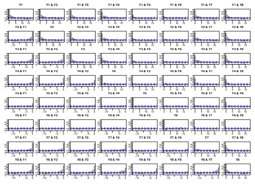
(a) Cross correlogram of the original $8$ differenced index series.

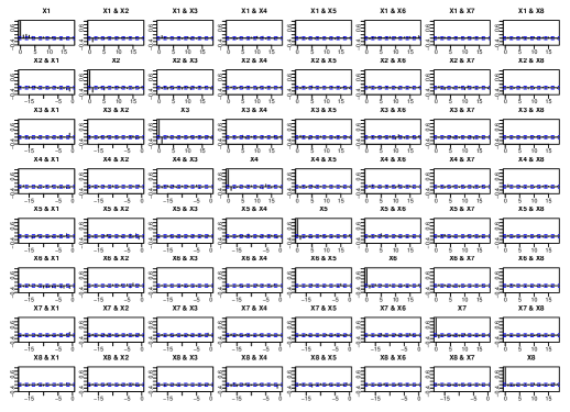
(b) Cross correlogram of the $8$ transformed component time series.

Figure 2: Cross correlograms for Example 2.

Example 3.

We consider the weekly notified measles cases in 7 cities in England (i.e. London, Bristol, Liverpool, Manchester, Newcastle, Birmingham and Sheffield) in 1948 – 1965, before the advent of vaccination. All the 7 series show biennial cycles, which is a common feature in measles dynamics in the pre-vaccination period. This biennial cycling is the major driving force for the cross correlations among different component series displayed in Fig 3(a). The cross correlogram of the transformed data is displayed in Fig 3(b). Since none of the transformed component series are white noise, the confidence bounds in Fig 3(b) could be misleading; see Remark 1(i).

(a) Cross correlogram of the original $7$ measles series.

(b) Cross correlogram of the $7$ transformed component time series.

Figure 3: Cross correlograms for Example 3.

We apply prewhitening to each transformed component time series by fitting an AR model with the order determined by AIC and with the maximum order set at 5. Although all those 7 filtered time series behave like white noise, there are still quite a few small but significant cross correlations here and there. Fig 4(a) plots, in descending order, the maximum cross correlations $\widehat{L}_{n}(i,j)$ defined in (2.11) for those 7 transformed and prewhitened series. As $1.96/\sqrt{n}=0.064$ with $n=937$ now, one may argue that the segmentation assumption does not hold for this example. Consequently the ratio estimator $\widehat{r}$ defined in (2.12) does not make any sense for this example; see also Fig 4(b).

Nevertheless Fig 4(a) ranks the pairs of transformed component series according to the strength of the cross correlation. If we would only accept $r$ connected pairs, this leads to an approximate segmentation according to the rule set in Section 2.2.1. By doing this, we effectively ignore some small, though still statistically significant, cross correlations. Table2 lists the different segmentations corresponding to the different values of $r$. It shows that the group {4, 5} is always present until all the 7 series merge together. Further it only takes 6 connected pairs, corresponding to the 6 largest points in Fig 4(a), to merge all the series together.

Figure 4: (a) The maximum cross correlations, plotted in descending order, among each of the $({7\atop 2})=21$ pairs component series of the transformed and prewhitened measles series. The maximization was taken over the lags between -20 to 20. (b) The ratios of two successive correlations in (a).

Table 2: Segmentations determined by different numbers of connected pairs for the transformed series in Example 3.

No. of connected pairs	No. of groups	Segmentation
1	6	{4, 5}, {1}, {2}, {3}, {6}, {7}
2	5	{1, 2}, {4, 5}, {3}, {6}, {7}
3	4	{1, 2, 3}, {4, 5}, {6}, {7}
4	3	{1, 2, 3, 7}, {4, 5}, {6}
5	2	{1, 2, 3, 6, 7}, {4, 5}
6	1	{$1,\ldots,7$}

The forecasting comparison is conducted in the same manner as in Examples 1 and 2. We adopt the segmentation with 4 groups: {1, 2, 3}, {4, 5}, {6} and {7}, i.e. we regard that only the three pairs, corresponding to the 3 maximum cross correlations in Fig 4(a), are connected. We forecast the notified measles cases in the last 14 weeks of the period for all the 7 cities. Due to the fact that the data from different cities are on different scales, we present the results based on relative MSEs in Table1. More specifically, we first fit an AR model for each component series of the original time series and calculate the associated MSEs. For a given other method, we define its relative MSE for each component series of the original time series as the ratio of its MSE and that of the fitted univariate AR model mentioned before. Once again the forecasting based on this (approximate) segmentation is much more accurate than those based on the direct VAR and RVAR models, and univariate AR model to each of the original time series, although we have ignored quite a few small but significant cross correlations among the transformed series. The over-segmentation case with each component as an individual group and the incomplete-segmentation case with 3 groups ({1, 2, 3, 7}, {4, 5},{6}) are also considered. The over-segmentation ignores all the correlations between any different components of the transformed series. Such cross correlations in this example are very significant. Hence, the over-segmentation will have an adverse effect while the incomplete-segmentation taking account of more correlations will have an advantage in this case, which is also verified by the results presented in Table1.

Example 4.

Now we consider the daily log-sales of a clothing brand in 25 provinces in China in 1 January 2008 – 9 December 2012 (i.e. $n=1805$ and $p=25$). All those series exhibit peaks before the Spring Festival (i.e. the Chinese New Year, typically around February). The cross correlogram of the 8 randomly selected component series in Fig 5 indicates the strong cross correlations over different time lags among the sales over different provinces. The strong periodic components with the period 7 indicate a regular sales pattern over 7 different weekdays. By applying the proposed segmentation transformation and the permutation based on the maximum cross correlations with $m=25$ in (2.11), the transformed 25 time series are divided into 24 group with only non-single-element group containing the 15th and the 16th transformed series. The same grouping is obtained for $m$ between 14 and 30. Note for this example, we should not use small $m$ as the autocorrelations of the original data decay slowly; see Fig 5.

Figure 5: Cross correlogram of the log-sales series of 8 randomly selected provinces in Example 4.

To compare the post-sample forecasting performance, we calculate one-step-ahead and two-step-ahead forecasts for each of the daily log-sales in the last two weeks of the period. Table1 list the means and the standard deviations of the MSEs across the 25 provinces. With $p=25$, the fitted VAR(2) model, selected by AIC, contain $2\times 25\times 25=1250$ parameters, leading to poor post-sample forecasting. The RVAR(2) model improves the forecasting a bit, but it is still significantly worse than the forecasting based on the approach of fitting a univariate AR model to each of the original series directly. Since the proposed segmentation leads to 24 subseries, it also fits univariate AR models to 23 (out of 25) transformed series, fits a 2-dimensional VAR model to the 15th and the 16th transformed series together. The proposed approach leads to much more accurate forecasts as both the mean and standard deviation are much smaller than those of the other three methods. The above comparison shows clearly that the cross correlations in the sales over different provinces are valuable information which can improve the forecasting for the future sales significantly. However the endeavour to reduce the dimension by, for example, TS-PCA, is necessary in order to make use of this valuable information. We also consider an over-segmentation by regarding each component of the transformed series as an individual group, and an incomplete-segmentation with {5, 15, 16} as a group and the other $23$ components as $23$ individual groups. Both of them have good performance.

5 Segmenting multivariate volatility processes

The methodology proposed in Section 2 can be readily extended to segment multivariate volatility processes. To this end, let ${\mathbf{y}}_{t}$ be a $p\times 1$ volatility process. Let $\mathcal{F}_{t}=\sigma({\mathbf{y}}_{t},{\mathbf{y}}_{t-1},\ldots)$ and $\mbox{Var}({\mathbf{y}}_{t}|\mathcal{F}_{t-1})=\boldsymbol{\Sigma}_{y}(t)$. Without loss of generality, we assume $\mathbb{E}({\mathbf{y}}_{t}|\mathcal{F}_{t-1})={\mathbf{0}}$ and $\mbox{Var}({\mathbf{y}}_{t})={\mathbf{I}}_{p}$. Suppose that there exists an orthogonal matrix ${\mathbf{A}}$ for which ${\mathbf{y}}_{t}={\mathbf{A}}{\mathbf{x}}_{t}$ and $\mbox{Var}({\mathbf{x}}_{t}|\mathcal{F}_{t-1})={\rm diag}\{\boldsymbol{\Sigma}_{1}(t),\ldots,\boldsymbol{\Sigma}_{q}(t)\}$ with $\boldsymbol{\Sigma}_{1}(t),\ldots,\boldsymbol{\Sigma}_{q}(t)$ being, respectively, $p_{1}\times p_{1},\ldots,$ $p_{q}\times p_{q}$ non-negative definite matrices. Hence the latent $p$-dimensional volatility process ${\mathbf{x}}_{t}$ can be segmented into $q$ lower-dimensional processes, and there exist no conditional cross correlations across those $q$ processes.

Let ${\mathbf{W}}_{y}=\sum_{B\in\mathcal{B}_{t-1}}[\mathbb{E}\{{\mathbf{y}}_{t}{\mathbf{y}}_{t}^{\mathrm{\scriptscriptstyle T}}\mathbb{I}(B)\}]^{2}$ and ${\mathbf{W}}_{x}=\sum_{B\in\mathcal{B}_{t-1}}[\mathbb{E}\{{\mathbf{x}}_{t}{\mathbf{x}}_{t}^{\mathrm{\scriptscriptstyle T}}\mathbb{I}(B)\}]^{2},$ where $\mathcal{B}_{t-1}$ is a $\pi$-class and the $\sigma$-field generated by $\mathcal{B}_{t-1}$ equals to $\mathcal{F}_{t-1}$. Since it holds for any $B\in\mathcal{B}_{t-1}$ that $\mathbb{E}\{{\mathbf{x}}_{t}{\mathbf{x}}_{t}^{\mathrm{\scriptscriptstyle T}}\mathbb{I}(B)\}=\mathbb{E}\{\mathbb{I}(B)\mathbb{E}({\mathbf{x}}_{t}{\mathbf{x}}_{t}^{\mathrm{\scriptscriptstyle T}}|\mathcal{F}_{t-1})\}=\mathbb{E}[\mathbb{I}(B){\rm diag}\{\boldsymbol{\Sigma}_{1}(t),\ldots,\boldsymbol{\Sigma}_{q}(t)\}]$ is a block diagonal matrix, so is ${\mathbf{W}}_{x}$. Now (2.6) still holds for the newly defined ${\mathbf{W}}_{y}$ and ${\mathbf{W}}_{x}$. Thus ${\mathbf{A}}$ can be estimated exactly in the same manner as in Section 2.1. An estimator for ${\mathbf{W}}_{y}$ can be defined as $\widehat{\mathbf{W}}_{y}=\sum_{B\in\mathcal{B}}\sum_{k=1}^{k_{0}}\{(n-k)^{-1}\sum_{t=k+1}^{n}{\mathbf{y}}_{t}{\mathbf{y}}_{t}^{\mathrm{\scriptscriptstyle T}}\mathbb{I}({\mathbf{y}}_{t-k}\in B)\}^{2},$ where $\mathcal{B}$ is a set with elements $\{{\mathbf{u}}\in\mathbb{R}^{p}:\|{\mathbf{u}}\|_{2}\leq\|{\mathbf{y}}_{t}\|_{2}\}$ for $t=1,\ldots,n$. See Fan, Wang and Yao (2008). We illustrate this idea by a real data example.

Example 5.

We consider the daily returns of the stocks of Walt Disney Company, Wells Fargo $\&$ Company, Honeywell International Inc., MetLife Inc., H $\&$ R Block Inc. and Cognizant Technology Solutions Corporation in 14 July 2008 – 11 July 2014. For this data set, $n=1509$ and $p=6$. Denote by ${\mathbf{y}}_{t}=(y_{1,t},\ldots,y_{6,t})^{\mathrm{\scriptscriptstyle T}}$ the returns on the $t$-th day. By fitting each return series a GARCH(1,1) model, we calculate the residuals ${\varepsilon}_{i,t}=y_{i,t}/\widehat{\sigma}_{i,t}$ for $i=1,\ldots,6$, where $\widehat{\sigma}_{i,t}$ denotes the predicted volatility for the $i$-th return at time $t$ based on the fitted GARCH(1,1) model. The cross correlogram of the residual series are plotted in Fig 6(a), which shows the strong and significant concurrent correlations across all residual series. It indicates clearly that $\mbox{Var}({\mathbf{y}}_{t}|\mathcal{F}_{t-1})$ is not a block diagonal matrix. We also apply the traditional PCA to the 6 returns series, the cross correlogram of pre-whitened series is shown in Fig 6(b). There are also strong and significant concurrent correlations across the residual series, see Panels (1, 2), (2, 3), (3, 4), (2, 5) and (6, 4). This indicates all the principal components should not be modelled separately. Now we apply the segmentation transform stated above. We repeat the whitening process above for the transformed series $\widehat{\mathbf{x}}_{t}$, i.e. fit an GARCH(1,1) model for each of the component series of $\widehat{\mathbf{x}}_{t}$ and calculate the residuals. Fig 7 presents the cross correlogram of these new residual series. There exist almost no significant cross correlations among the residual series. This is the significant evidence to support the assertion that $\mbox{Var}({\mathbf{x}}_{t}|\mathcal{F}_{t-1})$ is a diagonal matrix. For this example, the segmentation method leads to the conditional uncorrelated components of Fan, Wang and Yao (2008).

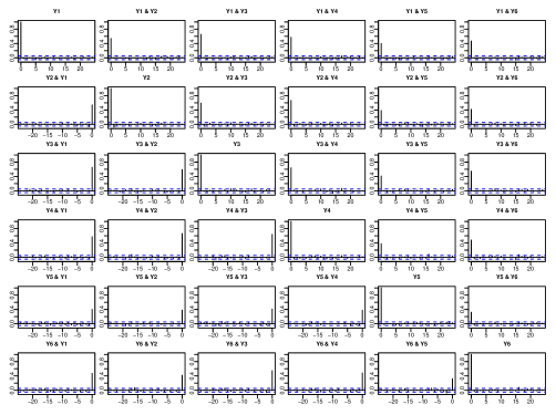
(a) Cross correlogram of the residuals resulted from fitting each original component series a GARCH(1,1) model.

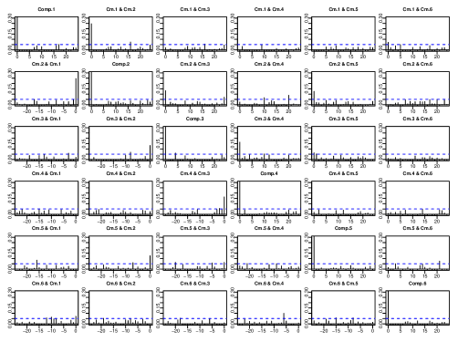
(b) Cross correlogram of the residuals resulted from fitting each series of PCA components a GARCH(1,1) model.

Figure 6: Cross correlograms for Example 5.

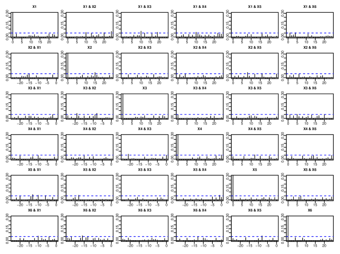
Figure 7: Cross correlogram of the residuals resulted from fitting each component series of the transformed series $\widehat{\mathbf{x}}_{t}$ with a GARCH(1,1) model in Example 5.

6 Final remarks

This paper proposes a contemporaneous linear transformation to segment a multiple time series into several both contemporaneously and serially uncorrelated subseries. The method is simple, and can be used as a preliminary step to reduce a high-dimensional time series modelling problem into several lower-dimensional problems. The reduction of dimensionality is often substantial and effective.

The method is abbreviated as TS-PCA, as it can be viewed as a version of PCA for multiple time series. Like the standard PCA, TS-PCA technically also boils down to an eigenanalysis for a positive definite matrix. The difference is that the intended segmentation is not guaranteed to exist. However one of the strengths of the proposed TS-PCA is that even when the segmentation assumption is invalid, it provides some approximate segmentations which ignore some minor (though still significant) cross correlations and, thus, lead to parsimonious modelling strategies. Those parsimonious strategies often bring in improvements in, for example, forecasting future values. See, e.g., Example 3. Furthermore when the dimension of time series is large, TS-PCA is necessary in order to use the information across different component series effectively. See, e.g., Example 4.

We have conducted some post-sample forecasting comparison with several real data including some not reported in the paper. The forecasting based on the proposed TS-PCA always outperforms that for the original data. We give one explanation as follows. It follows from (2.6) that $\Omega\equiv\mbox{tr}({\mathbf{W}}_{y})-p=\sum_{k=1}^{k_{0}}\sum_{i,j=1}^{p}\rho_{y,ij}^{2}(k)=\mbox{tr}({\mathbf{W}}_{x})-p=\sum_{k=1}^{k_{0}}\sum_{i,j=1}^{p}\rho_{x,ij}^{2}(k),$ where $\rho_{y,ij}(k)$ and $\rho_{x,ij}(k)$ denote, respectively, the cross correlation at lag $k$ between the $i$-th and the $j$-th components of ${\mathbf{y}}_{t}$ and ${\mathbf{x}}_{t}$. Since the future prediction is based on the serial correlations, $\Omega$ defined above can be taken as a measure for the predictive strength, which is the same for ${\mathbf{y}}_{t}$ and ${\mathbf{x}}_{t}$. To make use the full predictive strength of ${\mathbf{y}}_{t}$, we need to model the $p$-vector process appropriately to catch all the autocorrelations and cross-correlations (over different time lags) among the $p$ components of ${\mathbf{y}}_{t}$. In contrast, such a task for ${\mathbf{x}}_{t}$ is much easier as it can be divided into $q$ lower-dimensional problems. In the ideal situation when $q=p$, i.e. $\rho_{x,ij}(k)=0$ for any $i\neq j$, we just need to model all the component series of ${\mathbf{x}}_{t}$ separately in order to make the full use of the overall predictive strength.

References

- Anderson (1963) Anderson, T. W. (1963). The use of factor analysis in the statistical analysis of multiple time series. Psychometrika, 28, 1–25.
- Back and Weigend (1997) Back, A. D. and Weigend, A. S. (1997). A first application of independent component analysis to extracting structure from stock returns. Int. J. Neural Syst., 8, 473–484.
- Bai and Ng (2002) Bai, J. and Ng, S. (2002). Determining the number of factors in approximate factor models. Econometrica, 70, 191–221.
- Belouchrani et al. (1997) Belouchrani, A., Abed-Meraim, K., Cardoso, J.-F. and Moulines, E. (1997). A blind source separation technique using second-order statistics. IEEE T. Signal Proces., 45, 434–444.
- Bickel and Levina (2008) Bickel, P. J. and Levina, E. (2008). Covariance regularization by thresholding. Ann. Stat., 36, 2577–2604.
- Box and Jenkins (1970) Box, G. E. P. and Jenkins, G. M. (1970). Time Series Analysis, Forecasting and Control. Holden-Day, San Francisco.
- Box and Tiao (1977) Box, G. E. P. and Tiao, G. C. (1977). A canonical analysis of multiple time series. Biometrika, 64, 355–365.
- Brockwell and Davis (1996) Brockwell, P. J. and Davis, R. A. (1996). Introduction to Time Series and Forecasting. Springer, New York.
- Brillinger (1981) Brillinger, D. R. (1981). Time Series: Data Analysis and Theory. Holt, Rinehart and Winston, New York.
- Cardoso (1998) Cardoso, J. (1998). Multidimensional independent component analysis. Proceedings of the 1998 IEEE Int. Conf. Acoustics, Speech and Signal Processing, 4, 1941–1944.
- Chang, Guo and Yao (2015) Chang, J., Guo, B. and Yao, Q. (2015). High dimensional stochastic regression with latent factors, endogeneity and nonlinearity. J. Econometrics, 189, 297–312.
- Chang, Guo and Yao (2016) Chang, J., Guo, B. and Yao, Q. (2016). Supplement to “Principal component analysis for second-order stationary vector time series.”
- Davis, Zang and Zheng (2012) Davis, R. A., Zang, P. and Zheng, T. (2012). Sparse vector autoregressive modelling. Available at arXiv:1207.0520.
- Fan, Wang and Yao (2008) Fan, J., Wang, M. and Yao, Q. (2008). Modelling multivariate volatilities via conditionally uncorrelated components. J. Roy. Stat. Soc. B., 70, 679–702.
- Fan and Yao (2003) Fan, J. and Yao, Q. (2003). Nonlinear Time Series: Nonparametric and Parametric Methods. Springer, New York.
- Forni et al. (2005) Forni, M., Hallin, M., Lippi, M. and Reichlin, L. (2005). The generalized dynamic factor model: One-sided estimation and forecasting. J. Am. Stat. Assoc., 100, 830–840.
- Guo, Wang and Yao (2016) Guo, S., Wang, Y. and Yao, Q. (2016). High-dimensional and banded vector autoregressions. Biometrika, 103, 889–903.
- Han and Liu (2013) Han, F. and Liu, H. (2013). A direct estimation of high dimensional stationary vector autoregressions. Available at arXiv:1307.0293.
- Huang and Tsay (2014) Huang, D. and Tsay, R. S. (2014). A refined scalar component approach to multivariate time series modeling. Manuscript.
- Hyvärinen, Karhunen and Oja (2001) Hyvärinen, A., Karhunen, J. and Oja, E. (2001). Independent Component Analysis. Wiley, New York.
- Jakeman, Steele and Young (1980) Jakeman, A. J., Steele, L. P. and Young, P. C. (1980). Instrumental variable algorithms for multiple input systems described by multiple transfer functions. IEEE T. Syst. Man. Cyb., 10, 593–602.
- Lam, Yao and Bathia (2011) Lam, C., Yao, Q. and Bathia, N. (2011). Estimation of latent factors for high-dimensional time series. Biometrika, 98, 901–918.
- Lam and Yao (2012) Lam, C. and Yao, Q. (2012). Factor modeling for high-dimensional time series: inference for the number of factors. Ann. Stat., 40, 694–726.
- Ledoit and Wolf (2004) Ledoit, O. and Wolf, M. (2004). A well-conditioned estimator for large-dimensional covariance matrices. J. Multivariate Anal., 88, 356–411.
- Liu, Xiao and Wu (2013) Liu, W., Xiao, H. and Wu, W. B. (2013). Probability and moment inequalities under dependence. SS, 23, 1257–1272
- Lütkepohl (2006) Lütkepohl, H. (2006). New Introduction to Multiple Time Series Analysis. Springer, Berlin.
- Matteson and Tsay (2011) Matteson, D. S. and Tsay, R. S. (2011). Dynamic orthogonal components for multivariate time series. J. Am. Stat. Assoc., 106, 1450–1463.
- Pan and Yao (2008) Pan, J. and Yao, Q. (2008). Modelling multiple time series via common factors. Biometrika, 95, 365–379.
- Paparoditis and Politis (2012) Paparoditis and Politis (2012). Nonlinear spectral density estimation: thresholding the correlogram. J. Time Ser. Anal., 33, 386–397.
- Peña and Box (1987) Peña, D. and Box, G. E. P. (1987). Identifying a simplifying structure in time series. J. Am. Stat. Assoc., 82, 836–843.
- Reinsel (1993) Reinsel, G. C. (1993). Elements of Multivariate Time Series Analysis (2nd edition). Springer.
- Rio (2000) Rio, E. (2000). Théorie asymptotique des processus aléatoires faiblement dépendants. Springer, Berlin.
- Sarkar and Chang (1997) Sarkar, S. K. and Chang, C.-K. (1997). The Simes method for multiple hypothesis testing with positively dependent test statistics. J. Am. Stat. Assoc., 92, 1601–1608.
- Shojaie and Michailidis (2010) Shojaie, A. and Michailidis, G. (2010). Discovering graphical Granger causality using the truncated lasso penalty. Bioinformatics, 26, 517–523.
- Simes (1986) Simes, R. J. (1986). An improved Bonferroni procedure for multiple tests of significance. Biometrika, 73, 751–754.
- Song and Bickel (2011) Song, S. and Bickel, P. J. (2011). Large vector auto regressions. Available at arXiv:1106.3519.
- Stewart and Sun (1990) Stewart, G. W. and Sun, J. (1990). Matrix Perturbation Theory. Academic Press.
- Stock and Watson (2002) Stock, J. H. and Watson, M. W. (2002), Forecasting using principal components from a large number of predictors. J. Am. Stat. Assoc., 97, 1167–1179.
- Stock and Watson (2005) Stock, J. H. and Watson, M. W. (2005). Implications of dynamic factor models for VAR analysis. Available at www.nber.org/papers/w11467.
- Theis, Meyer-Baese and Lang (2004) Theis, F. J., Meyer-Baese, A. and Lang, E. W. (2004). Second-order blind source separation based on multi-dimensional autocovariances. In Independent Component Analysis and Blind Signal Separation (Edi. C.G. Puntonet and A. Prieto). Springer, 726-733.
- Tiao and Tsay (1989) Tiao, G. C. and Tsay, R. S. (1989). Model specification in multivariate time series (with discussion). J. Roy. Stat. Soc. B., 51, 157–213.
- Tong, Xu and Kailath (1994) Tong, L. Xu, G. and Kailath, T. (1994). Blind identification and equalization based on second-order statistics: a time domain approach. IEEE T. Inform. Theory, 40, 340–349.
- Tsay (2014) Tsay, R. (2014). Multivariate Time Series Analysis. Wiley.