Low Mach Number Fluctuating Hydrodynamics of Binary Liquid Mixtures

Abstract

Continuing on our previous work [A. Donev, A. Nonaka, Y. Sun, T. G. Fai, A. L. Garcia and J. B. Bell, Comm. App. Math. and Comp. Sci., 9-1:47-105, 2014], we develop semi-implicit numerical methods for solving low Mach number fluctuating hydrodynamic equations appropriate for modeling diffusive mixing in isothermal mixtures of fluids with different densities and transport coefficients. We treat viscous dissipation implicitly using a recently-developed variable-coefficient Stokes solver [M. Cai, A. J. Nonaka, J. B. Bell, B. E. Griffith and A. Donev, Commun. Comput. Phys., 16(5):1263-1297, 2014]. This allows us to increase the time step size significantly for low Reynolds number flows with large Schmidt numbers compared to our earlier explicit temporal integrator. Also, unlike most existing deterministic methods for low Mach number equations, our methods do not use a fractional time-step approach in the spirit of projection methods, thus avoiding splitting errors and giving full second-order deterministic accuracy even in the presence of boundaries for a broad range of Reynolds numbers including steady Stokes flow. We incorporate the Stokes solver into two time-advancement schemes, where the first is suitable for inertial flows and the second is suitable for the overdamped limit (viscous-dominated flows), in which inertia vanishes and the fluid motion can be described by a steady Stokes equation. We also describe how to incorporate advanced higher-order Godunov advection schemes in the numerical method, allowing for the treatment of (very) large Peclet number flows with a vanishing mass diffusion coefficient. We incorporate thermal fluctuations in the description in both the inertial and overdamped regimes. We validate our algorithm with a series of stochastic and deterministic tests. Finally, we apply our algorithms to model the development of giant concentration fluctuations during the diffusive mixing of water and glycerol, and compare numerical results with experimental measurements. We find good agreement between the two, and observe propagative (non-diffusive) modes at small wavenumbers (large spatial scales), not reported in published experimental measurements of concentration fluctuations in fluid mixtures. Our work forms the foundation for developing low Mach number fluctuating hydrodynamics methods for miscible multi-species mixtures of chemically reacting fluids.

I Introduction

Flows of realistic mixtures of miscible fluids exhibit several features that make them more difficult to simulate numerically than flows of simple fluids. Firstly, the physical properties of the mixture depend on the concentration of the different species composing the mixture. This includes both the density of the mixture at constant pressure, and transport coefficients such as viscosity and mass diffusion coefficients. Common simplifying assumptions such as the Boussinesq approximation, which assumes a constant density and thus incompressible flow, or assuming constant transport coefficients, are uncontrolled and not appropriate for certain mixtures of very dissimilar fluids. Secondly, for liquid mixtures there is a large separation of time scales between the various dissipative processes, notably, mass diffusion is much slower than momentum diffusion. The large Schmidt numbers $\mbox{Sc}\sim 10^{3}-10^{4}$ typical of liquid mixtures lead to extreme stiffness and make direct temporal integration of the hydrodynamic equations infeasible. Lastly, flows of mixtures exhibit all of the numerical difficulties found in single component flows, for example, well-known difficulties caused by advection in the absence of sufficiently strong dissipation (diffusion of momentum or mass), and challenges in incorporating thermal fluctuations in the description. Here we develop a low Mach number approach to isothermal binary fluid mixtures that resolves many of the above difficulties, and paves the way for incorporating additional physics such as the presence of more than two species MultispeciesCompressible , chemical reactions MultispeciesChemistry ; DiffusiveInstability_Chemistry_PRL , multiple phases and surface tension StagerredFluct_Inhomogeneous ; CHN_Compressible , and others.

Stochastic fluctuations are intrinsic to fluid dynamics because fluids are composed of molecules whose positions and velocities are random. Thermal fluctuations affect flows from microscopic to macroscopic scales DiffusionRenormalization_PRL ; FractalDiffusion_Microgravity and need to be consistently included in all levels of description. Fluctuating hydrodynamics (FHD) incorporates thermal fluctuations into the usual Navier-Stokes-Fourier laws in the form of stochastic contributions to the dissipative momentum, heat, and mass fluxes FluctHydroNonEq_Book . FHD has proven to be a very useful tool in understanding complex fluid flows far from equilibrium LB_SoftMatter_Review ; StagerredFluct_Inhomogeneous ; LB_OrderParameters ; SELM ; however, theoretical calculations are often only feasible after making many uncontrolled approximations FluctHydroNonEq_Book , and numerical schemes used for fluctuating hydrodynamics are usually far behind state-of-the-art deterministic computational fluid dynamics (CFD) solvers.

In this work, we consider binary mixtures and restrict our attention to isothermal flows. We consider a specific equation of state (EOS) suitable for mixtures of incompressible liquids or ideal gases, but otherwise account for advective and diffusive mass and momentum transport in full generality. Recently, some of us developed finite-volume methods for the incompressible equations LLNS_Staggered . We have also developed low Mach number isothermal fluctuating equations LowMachExplicit , which eliminate the stiffness arising from the separation of scales between acoustic and vortical modes IncompressibleLimit_Majda ; ZeroMach_Buoyancy ; ZeroMachCombustion . The low Mach number equations account for the fact that for mixtures of fluids with different densities, diffusive and stochastic mass fluxes create local expansion and contraction of the fluid. In these equations the incompressibility constraint should be replaced by a “quasi-incompressibility” constraint ZeroMachCombustion ; Cahn-Hilliard_QuasiIncomp , which introduces some difficulties in constructing conservative finite-volume techniques LowMachAdaptive ; ZeroMach_Klein ; LaminarFlowChemistry ; LowMach_FiniteDifference ; LowMachAcoustics ; LowMachExplicit . In Section II we review the low Mach number equations of fluctuating hydrodynamics for a binary mixture of miscible fluids, as first proposed in Ref. LowMachExplicit .

The numerical method developed in Ref. LowMachExplicit uses an explicit temporal integrator. This requires using a small time step and is infeasible for liquid mixtures due to the stiffness caused by the separation of time scales between fast momentum diffusion and slow mass diffusion. In recent work MultiscaleIntegrators , some of us developed temporal integrators for the equations of fluctuating hydrodynamics that have several important advantages. Notably, these integrators are semi-implicit, allowing one to treat fast momentum diffusion (viscous dissipation) implicitly, and other transport processes explicitly. Furthermore, these temporal integrators are constructed to be second-order accurate for the equations of linearized fluctuating hydrodynamics (LFHD), which are suitable for describing thermal fluctuations around stable macroscopic flows over a broad range of length and time scales FluctHydroNonEq_Book . Importantly, the linearization of the fluctuating equations is carried out automatically by the code, making the numerical methods very similar to standard deterministic CFD schemes. Finally, specific integrators are proposed in Ref. MultiscaleIntegrators to handle the extreme separation of scales between the fast velocity and the slow concentration by taking an overdamped limit of the inertial equations. In this work, we extend the semi-implicit temporal integrators proposed in Ref. MultiscaleIntegrators for incompressible flows to account for the quasi-incompressible nature of low Mach number flows. We apply these temporal integrators to the staggered-grid conservative finite-volume spatial discretization developed in Ref. LowMachExplicit , and additionally generalize the treatment of advection to allow for the use of monotonicity-preserving higher-order Godunov schemes bellColellaGlaz:1989 ; BDS ; SemiLagrangianAdvection_2D ; SemiLagrangianAdvection_3D .

Our work relies heavily on several prior works, which we will only briefly summarize in the present paper. The spatial discretization we describe in more detail in Section III.2 is identical to that proposed by Donev et al LowMachExplicit , which itself relies heavily on the treatment of thermal fluctuations developed in Refs. LLNS_Staggered ; LowMachExplicit . A key development that makes the algorithm presented here feasible for large-scale problems is recent work by some of us StokesKrylov on efficient multigrid-based iterative methods for solving unsteady and steady variable-coefficient Stokes problems on staggered grids. Our high-order Godunov method for mass advection is based on the work of Bell et al. BDS ; SemiLagrangianAdvection_2D ; SemiLagrangianAdvection_3D .

The temporal integrators developed in Section III.4 are a novel approach to low Mach number hydrodynamics even in the deterministic context. In high-resolution finite-volume methods, the dominant paradigm has been to use a splitting (fractional-step) or projection method Chorin68 to separate the pressure and velocity updates almgren-iamr ; LaminarFlowChemistry ; LowMach_Nuclear ; LowMachSupernovae ; ZeroMach_Klein_2 . We followed such a projection approach to construct an explicit temporal integrator for the low Mach number equations LowMachExplicit . When viscosity is treated implicitly, however, the splitting introduces a commutator error that leads to the appearance of spurious or “parasitic” modes in the presence of physical boundaries GaugeIncompressible_E ; ProjectionMethods_Minion ; DFDB . There are several techniques to reduce (but not eliminate) these artificial boundary layers ProjectionMethods_Minion , and for sufficiently large Reynolds number flows the time step size dictated by advective stability constraints makes the splitting error relatively small in practice. At small Reynolds numbers, however, the splitting error becomes larger as viscous effects become more dominant, and projection methods do not apply in the steady Stokes regime for problems with physical boundary conditions. Methods that do not split the velocity and pressure updates but rather solve a combined Stokes system for velocity and pressure have been used in the finite-element literature for some time, and have more recently been used in the finite-volume context for incompressible flow NonProjection_Griffith . Here we demonstrate how the same approach can be effectively applied to the low Mach number equations for a binary fluid mixture LowMachExplicit , to construct a method that is second-order accurate up to boundaries, for a broad range of Reynolds numbers including steady Stokes flow.

We test our ability to accurately capture the static structure factor for equilibrium fluctuation calculations. Then, we test our methods deterministically on two variable density and variable viscosity low Mach number flows. First, we confirm second-order deterministic accuracy in both space and time for a lid-driven cavity problem in the presence of a bubble of a denser miscible fluid. Next, we simulate the development of a Kevin-Helmholtz instability as a lighter less viscous fluid streams over a denser more viscous fluid. These tests confirm the robustness and accuracy of the methods in the presence of large contrasts, sharp gradients, and boundaries. Next we focus on the use of fluctuating low Mach number equations to study giant concentration fluctuations. In Section V we apply our methods to study the development of giant fluctuations GiantFluctuations_Theory ; GiantFluctuations_Cannell ; FractalDiffusion_Microgravity ; GiantFluctuations_Summary during free diffusive mixing of water and glycerol. We compare simulation results to experimental measurements of the time-correlation function of concentration fluctuations during the diffusive mixing of water and glycerol GiantFluctuations_Cannell . The relaxation times show signatures of the rich deterministic dynamics, and a transition from purely diffusive relaxation of concentration fluctuations at large wavenumbers, to more complex buoyancy-driven dynamics at smaller wavenumbers. We find reasonably-good agreement given the large experimental uncertainties, and observe the appearance of propagative modes at small wavenumbers, which we suggest could be observed in experiments as well.

II Low Mach Number Equations

At mesoscopic scales, in typical liquids, sound waves are very low amplitude and much faster than momentum diffusion; hence, they can usually be eliminated from the fluid dynamics description. Formally, this corresponds to taking the zero Mach number singular limit $\mbox{Ma}\rightarrow 0$ of the well-known compressible fluctuating hydrodynamics equations system Landau:Fluid ; FluctHydroNonEq_Book . In the compressible equations, the coupling between momentum and mass transport is captured by the equation of state (EOS) for the pressure $P(\rho,c;T_{0})$ as a local function of the density $\rho(\boldsymbol{r},t)$ and mass concentration $c(\boldsymbol{r},t)$ at a specified temperature $T_{0}\left(\boldsymbol{r}\right)$, assumed to be time-independent in our isothermal model.

The low Mach number equations can be obtained by making the ansatz that the thermodynamic behavior of the system is captured by a reference pressure $P_{0}\left(\boldsymbol{r},t\right)$, with the additional pressure contribution $\pi\left(\boldsymbol{r},t\right)=O\left(\mbox{Ma}^{2}\right)$ capturing the mechanical behavior while not affecting the thermodynamics. We will restrict consideration to cases where stratification due to gravity causes negligible changes in the thermodynamic state across the domain. In this case, the reference pressure is spatially constant and constrains the system so that the evolution of $\rho$ and $c$ remains consistent with the thermodynamic EOS

$$P\left(\rho\left(\boldsymbol{r},t\right),c\left(\boldsymbol{r},t\right);T_{0}\left(\boldsymbol{r}\right)\right)=P_{0}\left(t\right).$$ (1)

Physically this means that any change in concentration must be accompanied by a corresponding change in density, as would be observed in a system at thermodynamic equilibrium held at the fixed reference pressure and temperature. The EOS defines density $\rho\left(c\left(\boldsymbol{r},t\right);T_{0}\left(\boldsymbol{r}\right),P_{0}\left(t\right)\right)$ as an implicit function of concentration in a binary liquid mixture. The EOS constraint (1) can be re-written as a constraint on the divergence of the fluid velocity $\boldsymbol{v}(\boldsymbol{r},t)$,

$$\rho\boldsymbol{\nabla}\cdot\boldsymbol{v}=-\beta\,\boldsymbol{\nabla}\cdot\boldsymbol{F},$$ (2)

where $\boldsymbol{F}$ is the total diffusive mass flux defined in (10), and the solutal expansion coefficient

$$\beta\left(c\right)=\frac{1}{\rho}\left(\frac{\partial\rho}{\partial c}\right)_{P_{0},T_{0}}$$

is determined by the specific form of the EOS.

In this work we consider a specific linear EOS,

$$\frac{\rho_{1}}{\bar{\rho}_{1}}+\frac{\rho_{2}}{\bar{\rho}_{2}}=\frac{c\rho}{\bar{\rho}_{1}}+\frac{(1-c)\rho}{\bar{\rho}_{2}}=1,$$ (3)

where $\bar{\rho}_{1}$ and $\bar{\rho}_{2}$ are the densities of the pure component fluids ($c=1$ and $c=0$, respectively), giving

$$\beta=\rho\left(\frac{1}{\bar{\rho}_{2}}-\frac{1}{\bar{\rho}_{1}}\right)=\frac{\bar{\rho}_{1}-\bar{\rho}_{2}}{c\bar{\rho}_{2}+(1-c)\bar{\rho}_{1}}.$$ (4)

It is important that for this specific form of the EOS $\beta/\rho$ is a material constant independent of the concentration; this allows us to write the EOS constraint (9) in conservative form $\boldsymbol{\nabla}\cdot\boldsymbol{v}=-\boldsymbol{\nabla}\cdot\left(\beta\rho^{-1}\boldsymbol{F}\right)$ and take the reference pressure $P_{0}$ to be independent of time. The specific form of the density dependence (4) on concentration arises if one assumes that two incompressible fluids do not change volume upon mixing, which is a reasonable assumption for liquids that are not too dissimilar at the molecular level. Surprisingly the EOS (3) is also valid for a mixture of ideal gases. If the specific EOS (3) is not a very good approximation over the entire range of concentration $0\leq c\leq 1$, (3) may be a very good approximation over the range of concentrations of interest if $\bar{\rho}_{1}$ and $\bar{\rho}_{2}$ are adjusted accordingly. Our choice of the specific form of the EOS will aid significantly in the construction of simple conservative spatial discretizations that strictly maintain the EOS without requiring complicated nonlinear iterative corrections.

In fluctuating hydrodynamics, stochastic contributions to the momentum and mass fluxes that are formally modeled as LLNS_Staggered

$$\boldsymbol{\Sigma}=\sqrt{\eta k_{B}T}\left(\boldsymbol{\mathcal{W}}+\boldsymbol{\mathcal{W}}^{T}\right)\mbox{ and } \boldsymbol{\Psi}=\sqrt{2\chi\rho\mu_{c}^{-1}k_{B}T}\;\widetilde{\boldsymbol{\mathcal{W}}},$$ (5)

where $k_{B}$ is Boltzmann’s constant, $\eta$ is the shear viscosity, $\chi$ is the diffusion coefficient, $\mu\left(c;T_{0},P_{0}\right)$ is the chemical potential of the mixture with $\mu_{c}=\left(\partial\mu/\partial c\right)_{P_{0},T_{0}}$, and $\boldsymbol{\mathcal{W}}(\boldsymbol{r},t)$ and $\widetilde{\boldsymbol{\mathcal{W}}}(\boldsymbol{r},t)$ are standard zero mean, unit variance random Gaussian tensor and vector fields, respectively, with uncorrelated components,

$$\langle\mathcal{W}_{ij}(\boldsymbol{r},t)\mathcal{W}_{kl}(\boldsymbol{r}^{\prime},t^{\prime})\rangle=\delta_{ik}\delta_{jl}\;\delta(t-t^{\prime})\delta(\boldsymbol{r}-\boldsymbol{r}^{\prime}),$$

and similarly for $\widetilde{\boldsymbol{\mathcal{W}}}$.

A standard asymptotic low Mach analysis IncompressibleLimit_Majda , formally treating the stochastic forcing as smooth, leads to the isothermal low Mach number equations for a binary mixture of fluids in conservation form LowMachExplicit ,

$$\partial_{t}\left(\rho\boldsymbol{v}\right)+\nabla\pi= -\boldsymbol{\nabla}\cdot\left(\rho\boldsymbol{v}\boldsymbol{v}^{T}\right)+\boldsymbol{\nabla}\cdot\left(\eta\bar{\boldsymbol{\nabla}}\boldsymbol{v}+\boldsymbol{\Sigma}\right)+\rho\boldsymbol{g}$$ (6)

$$\partial_{t}\left(\rho_{1}\right)= -\boldsymbol{\nabla}\cdot\left(\rho_{1}\boldsymbol{v}\right)+\boldsymbol{\nabla}\cdot\boldsymbol{F}$$ (7)

$$\partial_{t}\left(\rho_{2}\right)= -\boldsymbol{\nabla}\cdot\left(\rho_{2}\boldsymbol{v}\right)-\boldsymbol{\nabla}\cdot\boldsymbol{F}$$ (8)

$$\boldsymbol{\nabla}\cdot\boldsymbol{v}= -\boldsymbol{\nabla}\cdot\left(\beta\rho^{-1}\boldsymbol{F}\right),$$ (9)

where the deterministic and stochastic diffusive mass fluxes are denoted by

$$\boldsymbol{F}=\rho\chi\boldsymbol{\nabla}c+\boldsymbol{\Psi}.$$ (10)

Here $\bar{\boldsymbol{\nabla}}=\boldsymbol{\nabla}+\boldsymbol{\nabla}^{T}$ is a symmetric gradient, $\rho_{1}=\rho c$ is the density of the first component, $\rho_{2}=(1-c)\rho$ is the density of the second component, and $\boldsymbol{g}$ is the gravitational acceleration. The gradient of the non-thermodynamic component of the pressure $\pi$ (Lagrange multiplier) appears in the momentum equation as a driving force that ensures the EOS constraint (9) is obeyed. We note that the bulk viscosity term gives a gradient term that can be absorbed in $\pi$ and therefore does not explicitly need to appear in the equations. Temperature dynamics and fluctuations are neglected in these equations; however, this type of approach can be extended to include thermal effects. The shear viscosity $\eta\left(c;T_{0},P_{0}\right)$ and the mass diffusion coefficient $\chi\left(c;T_{0},P_{0}\right)$ in general depend on the concentration. Note that the two density equations (7,8) can be combined to obtain the usual continuity equation for the total density,

$$\partial_{t}\rho=-\boldsymbol{\nabla}\cdot\left(\rho\boldsymbol{v}\right),$$ (11)

and the primitive (non-conservation law) form of the concentration equation,

$$\rho\left(\partial_{t}c+\boldsymbol{v}\cdot\boldsymbol{\nabla}c\right)=\boldsymbol{\nabla}\cdot\boldsymbol{F}.$$ (12)

Our conservative numerical scheme is based on Eqs. (6,7,9,11).

In Ref. LowMachExplicit we discussed the effect of the low Mach constraint on the thermal fluctuations, suitable boundary conditions for the low Mach equations, and presented a gauge formulation of the equations that formally eliminates pressure in a manner similar to the projection operator formulation for incompressible flows. Importantly, the gauge formulation demonstrates that although the low Mach equations have the appearance of a constrained system, one can write them in an unconstrained form by introducing a gauge degree of freedom for the pressure. For the purposes of time integration, one can therefore treat these equations as standard initial-value problems LowMachExplicit and use the temporal integrators developed in Ref. MultiscaleIntegrators .

II.1 Linearized low Mach fluctuating hydrodynamics

It is important to note that the equations of fluctuating hydrodynamics should be interpreted as a mesoscopic coarse-grained representation of the mass, momentum and energy transport in fluids OttingerBook . As such, these equations implicitly contain a mesoscopic coarse-graining length and time scale that is larger than molecular scales DiscreteLLNS_Espanol and can only formally be written as stochastic partial differential equations (SPDEs). A coarse-graining scale can explicitly be included in the SPDEs DiffusionJSTAT ; DDFT_Hydro ; such a coarse-graining scale explicitly enters in our finite-volume spatio-temporal discretization through the grid spacing (equivalently, the volume of a grid cell, or more precisely, the number of molecules per grid cell). Additional difficulties are posed by the fact that in general the noise in the nonlinear equations is multiplicative, requiring a careful stochastic interpretation; the Mori-Zwanzig projection formalism GrabertBook suggests the correct stochastic interpretation is the kinetic one KineticStochasticIntegral_Ottinger .

For compressible and incompressible flows, the SPDEs of linearized fluctuating hydrodynamics (LFHD) FluctHydroNonEq_Book can be given a precise continuum meaning DaPratoBook ; LLNS_S_k ; DFDB ; MultiscaleIntegrators . In these linearized equations one splits each variable into a deterministic component and small fluctuations around the deterministic solution, e.g., $c\left(\boldsymbol{r},t\right)=\bar{c}\left(\boldsymbol{r},t\right)+\delta c\left(\boldsymbol{r},t\right)$, where $\bar{c}$ is a solution of the deterministic equations (6,7,9,11) with $\boldsymbol{\Psi}=0$ and $\boldsymbol{\Sigma}=0$. Here $\delta c$ is the solution of a linear additive-noise equation obtained by linearizing (12) to first order in the fluctuations and evaluating the noise amplitude at the deterministic solution; more precisely, LFHD is an expression of the central limit theorem in the limit of weak noise. In this work, in the stochastic setting we restrict our attention to LFHD equations. As discussed in Ref. MultiscaleIntegrators , we do not need to write down the (rather tedious) complete form of the linearized low Mach number equations (for an illustration, see Section II.2) since the numerical method will perform this linearization automatically. Namely, the complete nonlinear equations are essentially equivalent to the LFHD equations when the noise is sufficiently weak, i.e., when the hydrodynamic cells contain many molecules.

The low Mach number equations pose additional difficulties because they represent a coarse-graining of the dynamics not just in space but also in time. As such, even the linearized equations cannot directly be interpreted as describing a standard diffusion process. This is because the stochastic mass flux $\boldsymbol{\Psi}$ in the EOS constraint (9) makes the velocity formally white-in-time LowMachExplicit . We note, however, that the analysis in Ref. DiffusionJSTAT shows that there is a close connection between mass diffusion and advection by the thermally-fluctuating velocity field, and thus between $\boldsymbol{\Psi}$ and velocity fluctuations. This suggests that a precise interpretation of the low Mach constraint in the presence of stochastic mass fluxes requires a very delicate mathematical analysis. In this work we rely on the implicit coarse-graining in time provided by the finite time step size in the temporal integration schemes to regularize the low Mach equations LowMachExplicit . Furthermore, for the applications we study here, we can neglect stochastic mass fluxes and assume $\boldsymbol{\Psi}\approx 0$, in which case the difficulties related to a white-in-time velocity disappear.

II.2 Overdamped limit

At small scales, flows in liquids are viscous-dominated and the inertial momentum flux $\rho\boldsymbol{v}\boldsymbol{v}^{T}$ can often be neglected in a zero Reynolds number approximation. In addition, in liquids, there is a large separation of time scales between the fast momentum diffusion and slow mass diffusion, i.e., the Schmidt number $\mbox{Sc}=\eta/\left(\rho\chi\right)$ is large. This makes the relaxation times of velocity modes at sufficiently large wavenumbers much smaller than those of the concentration modes. Formally treating the stochastic force terms as smooth for the moment, the separation of time scales implies that we can replace the inertial momentum equation (6) with the overdamped steady-Stokes equation

$$-\boldsymbol{\nabla}\cdot\left(\eta\bar{\boldsymbol{\nabla}}\boldsymbol{v}\right)+\nabla\pi = \boldsymbol{\nabla}\cdot\boldsymbol{\Sigma}+\rho\boldsymbol{g}$$ (13)

$$\boldsymbol{\nabla}\cdot\boldsymbol{v} = -\left(\bar{\rho}_{2}^{-1}-\bar{\rho}_{1}^{-1}\right)\boldsymbol{\nabla}\cdot\left(\chi\rho\boldsymbol{\nabla}c+\boldsymbol{\Psi}\right).$$

The above equations can be used to eliminate velocity as a variable, leaving only the concentration equation (12). Note that the density equation (11) simply defines density as a function of concentration and thus is not considered an independent equation.

The solution of the Stokes system

$$-\boldsymbol{\nabla}\cdot\left(\eta\bar{\boldsymbol{\nabla}}\boldsymbol{v}\right)+\nabla\pi = \boldsymbol{f}$$ (14)

$$\boldsymbol{\nabla}\cdot\boldsymbol{v} = -h,$$

where $\boldsymbol{f}\left(\boldsymbol{r},t\right)$ and $h\left(\boldsymbol{r},t\right)$ are applied forcing terms, can be expressed in terms of a generalized inverse Stokes linear operator $\boldsymbol{\mathcal{L}}^{-1}\left[\eta\left(\cdot,t\right)\right]$ that is a functional of the viscosity (and thus the concentration),

$$\boldsymbol{v}=\boldsymbol{\mathcal{L}}^{-1}\left[\eta\right]\left(\boldsymbol{f},\,h\right).$$

In the linearized fluctuating equations, one must linearize around the (time dependent) solution of the deterministic nonlinear equation

$$\bar{\rho}\left(\partial_{t}\bar{c}+\bar{\boldsymbol{v}}\cdot\boldsymbol{\nabla}\bar{c}\right)=\boldsymbol{\nabla}\cdot\left(\bar{\rho}\bar{\chi}\boldsymbol{\nabla}\bar{c}\right),$$ (15)

where we have used the shorthand notation $\bar{\rho}=\rho\left(\bar{c}\right)$, $\bar{\eta}=\eta\left(\bar{c}\right)$, $\bar{\chi}=\chi\left(\bar{c}\right)$. Here the velocity is an implicit function of concentration defined via

$$-\boldsymbol{\nabla}\cdot\left(\bar{\eta}\bar{\boldsymbol{\nabla}}\boldsymbol{v}\right)+\nabla\bar{\pi} = \bar{\rho}\boldsymbol{g}$$

$$\boldsymbol{\nabla}\cdot\bar{\boldsymbol{v}} = -\left(\bar{\rho}_{2}^{-1}-\bar{\rho}_{1}^{-1}\right)\boldsymbol{\nabla}\cdot\left(\bar{\chi}\bar{\rho}\boldsymbol{\nabla}\bar{c}\right),$$

which we can write in shorthand notation as

$$\bar{\boldsymbol{v}}=\boldsymbol{\mathcal{L}}^{-1}\left[\bar{\eta}\right]\left(\bar{\rho}\boldsymbol{g},\;\left(\bar{\rho}_{2}^{-1}-\bar{\rho}_{1}^{-1}\right)\boldsymbol{\nabla}\cdot\left(\bar{\chi}\bar{\rho}\boldsymbol{\nabla}\bar{c}\right)\right).$$ (16)

Here we develop second-order integrators for the deterministic overdamped low Mach equation (15,16).

In the stochastic setting, the solution of (13) is white in time because the stochastic mass and momentum fluxes are white in time. This means that the advective term $\boldsymbol{v}\cdot\boldsymbol{\nabla}c$ requires a specific stochastic interpretation, in addition to the usual regularization (smoothing) in space required to interpet all nonlinear terms appearing in formal fluctuating hydrodynamics SPDEs. By performing a precise (albeit formal) adiabatic mode elimination of the fast velocity variable under the assumption of infinite separation of time scales, Donev et al. arrive at a Stratonovich interpretation of the random advection term $\boldsymbol{v}\cdot\boldsymbol{\nabla}c$ (see Appendix A of Ref. DiffusionJSTAT ). This analysis does not, however, directly extend to the low Mach number equations since it relies in key ways on the incompressibility of the fluid. Generalizing this sort of analysis to the case of variable fluid density is nontrivial, likely requiring the use of the gauge formulation of the low Mach equations, and appears to be beyond the scope of existing techniques. Variable (i.e., concentration-dependent) viscosity and mass diffusion coefficient can be handled using existing techniques although there are subtle nonlinear stochastic effects arising from the fact that the noise in the velocity equation is multiplicative and the invariant measure (equilibrium distribution) of the fast velocity depends on the slow concentration.

In the linearized setting, however, the difficulties associated with the interpretation of stochastic integrals and multiplicative noise disappear. The complete form of the linearized equations contains many terms and is rather tedious. Since we will never need to explicitly write this form let us illustrate the procedure by assuming $\chi$ and $\eta$ to be constant. For the concentration, we obtain the linearized equation

$$\bar{\rho}\left(\partial_{t}\left(\delta c\right)+\left(\delta\boldsymbol{v}\right)\cdot\boldsymbol{\nabla}\bar{c}\right)=\boldsymbol{\nabla}\cdot\left(\bar{\rho}\chi\boldsymbol{\nabla}\left(\delta c\right)+\bar{\rho}^{\prime}\chi\left(\boldsymbol{\nabla}\bar{c}\right)\delta c\right)-\bar{\rho}^{-1}\bar{\rho}^{\prime}\boldsymbol{\nabla}\cdot\left(\bar{\rho}\chi\boldsymbol{\nabla}\bar{c}\right)\delta c,$$ (17)

where $\bar{\rho}^{\prime}=d\rho\left(\bar{c}\right)/dc=\bar{\rho}\beta\left(\bar{\rho}\right)$ relates concentration fluctuations to density fluctuations via the EOS. Here we split $\delta\boldsymbol{v}=\delta\boldsymbol{v}_{c}+\delta\boldsymbol{v}_{f}$ into a component $\delta\boldsymbol{v}_{c}$ that is continuous in time and a component $\delta\boldsymbol{v}_{f}$ that is white in time,

$$\delta\boldsymbol{v}_{c} = \boldsymbol{\mathcal{L}}^{-1}\left[\bar{\eta}\right]\left(\bar{\rho}^{\prime}\boldsymbol{g}\delta c,\;\left(\bar{\rho}_{2}^{-1}-\bar{\rho}_{1}^{-1}\right)\boldsymbol{\nabla}\cdot\left(\bar{\rho}\chi\boldsymbol{\nabla}\left(\delta c\right)\right)\right),$$

$$\delta\boldsymbol{v}_{f} = \boldsymbol{\mathcal{L}}^{-1}\left[\bar{\eta}\right]\left(\boldsymbol{\nabla}\cdot\boldsymbol{\Sigma},\;\boldsymbol{\nabla}\cdot\boldsymbol{\Psi}\right).$$

The term $\bar{\rho}\left(\delta\boldsymbol{v}_{f}\right)\cdot\boldsymbol{\nabla}\bar{c}$ in (17) is interpreted as an additive noise term with a rather complicated and potentially time-dependent (via $\bar{\eta}\left(\bar{c}\left(\boldsymbol{r},t\right)\right)$) spatial correlation structure. In this work we develop numerical methods that solve the overdamped linearized equation (17) to second-order weakly MultiscaleIntegrators .

III Spatio-Temporal Discretization

Our baseline spatio-temporal discretization of the low Mach equations is based on the method of lines approach where we first discretize the (S)PDEs in space to obtain a system of (S)ODEs, which we then solve using a single-step multi-stage temporal integrator. The conservative finite-volume spatial discretization that we employ here is essentially identical to that developed in our previous works LowMachExplicit and StokesKrylov . In summary, scalar fields such as concentration and densities are cell-centered, while velocity is face-centered. In order to ensure conservation, the conserved momentum $\rho\boldsymbol{v}$ and mass densities $\rho_{1}$ and $\rho$ are evolved rather than the primitive variables $\boldsymbol{v}$ and $c$. Diffusion of mass and momentum is discretized using standard centered differences, leading to compact stencils similar to the standard Laplacian. Stochastic mass fluxes are associated with the faces of the regular grid, while for stochastic momentum fluxes we associate the diagonal elements with the cell centers and the off-diagonal elements with the nodes (in 2D) or edges (in 3D) of a regular grid with grid spacing $\Delta x$.

Here we focus our discussion on three new aspects of our spatio-temporal discretization. After summarizing the dimensionless numbers that control the appropriate choice of advection method and temporal integrator, in Section III.2 we describe our implementation of two advection schemes and a discussion of the advantages of each. In Section III.3 we describe our implicit treatment of viscous dissipation using a GMRES solver for the coupled velocity-pressure Stokes system. In Section III.4 we describe our overall temporal discretization strategies for the inertial and overdamped regimes.

III.1 Dimensionless Numbers

The suitability of a particular temporal integrator or advection scheme depends on the following dimensionless numbers:

cell Reynolds number $$\mbox{Re}_{c}=\frac{U\Delta x}{\nu}$$

cell Peclet number $$\mbox{Pe}_{c}=\frac{U\Delta x}{\chi}$$

Schmidt number $$\mbox{Sc}=\frac{\nu}{\chi}=\frac{\mbox{Pe}}{\mbox{Re}},$$

where $\nu=\eta/\rho$ is the kinematic viscosity. Observe that the first two depend on the spatial resolution and the typical flow speed $U$, while the Schmidt number is an intrinsic material property of the mixture. Also note that the physically relevant Reynolds Re and Peclet Pe numbers would be defined with a length scale much larger than $\Delta x$, such as the system size, and thus would be much larger than the discretization-scale numbers above. In this work, we are primarily interested in small-scale flows with $\mbox{Re}_{c}\lesssim 1$ and large Sc (liquid mixtures).

The choice of advection scheme for concentration (partial densities) is dictated by $\mbox{Pe}_{c}$. If $\mbox{Pe}_{c}\gtrsim 2$, centered advection schemes will generate non-physical oscillations, and one must use the Godunov advection scheme described below. However, it is important to note that in this case the spectrum of fluctuations will not be correctly preserved by the advection scheme; if fluctuations need to be resolved it is advisable to instead reduce the grid spacing and thus reduce the cell Peclet number to $\mbox{Pe}_{c}\lesssim 2$ and use centered advection.

The choice of the temporal integrator, on the other hand, is determined by the importance of inertia and the time scale of interest. If $\mbox{Re}_{c}$ is not sufficiently small, then there is no alternative to resolving the inertial dynamics of the velocity. Now let us assume that $Re\ll 1$, i.e., viscosity is dominant. If the time scale of interest is the advective timescale $L/U$, where $L$ is the system size, then one should use the inertial equations. However, the inertial temporal integrator described in Section III.4 will be rather inefficient if the time scale of interest is the diffusive time scale $L^{2}/\chi$, as is the case in the study of diffusive mixing presented in Section V. This is because the Crank-Nicolson (implicit midpoint) scheme used to treat viscosity in our methods is only A-stable, and, therefore, if the viscous Courant number $\nu\Delta t/\Delta x^{2}$ is too large, unphysical oscillations in the solution will appear (note that this problem is much more serious for fluctuating hydrodynamics due to the presence of fluctuations at all scales). In order to be able to use a time step size on the diffusive time scale, one must construct a stiffly accurate temporal integrator. This requires using an L-stable scheme to treat viscosity, such as the backward Euler scheme, which is however only first-order accurate.

Constructing a second-order stiffly accurate implicit-explicit integrator in the context of variable density low Mach flows is rather nontrivial. Furthermore, using an L-stable scheme leads to a damping of the velocity fluctuations at large wavenumbers and is inferior to the implicit midpoint scheme in the context of fluctuating hydrodynamics DFDB . Therefore, in this work we choose to consider separately the overdamped limit $\mbox{Re}\rightarrow 0$ and $\mbox{Sc}\rightarrow\infty$ (note that the value of Pe is arbitrary). In this limit we analytically eliminate the velocity as an independent variable, leaving only the concentration equation, which evolves on the diffusive time scale. We must emphasize, however, that the overdamped equations should be used with caution, especially in the presence of fluctuations. Notably, the validity of the overdamped approximation requires that the separation of time scales between the fast velocity and slow concentration be uniformly large over all wavenumbers, since fluctuations are present at all lengthscales. In the study of giant fluctuations we present in Section V, buoyancy effects speed up the dynamics of large-scale concentration fluctuations and using the overdamped limit would produce physically incorrect results at small wavenumbers. In microgravity, however, the overdamped limit is valid and we have used it to study giant fluctuations over very long time scales in a number of separate works GRADFLEXTransient ; DiffusionJSTAT .

III.2 Advection

We have implemented two advection schemes for cell-centered scalar fields, and describe under what conditions each is more suitable. The first is a simpler non-dissipative centered advection discretization described in our previous work LowMachExplicit . This scheme preserves the skew-adjoint nature of advection and thus maintains fluctuation-dissipation balance in the stochastic context. However, when sharp gradients are present, centered advection schemes require a sufficient amount of dissipation (diffusion) in order to avoid the appearance of Gibbs-phenomenon instabilities. Higher-order Godunov schemes have been used successfully with cell-centered finite volume schemes for some time bellColellaGlaz:1989 ; BDS ; SemiLagrangianAdvection_2D ; SemiLagrangianAdvection_3D . In these semi-Lagrangian advection schemes, a construction based on characteristics is used to estimate the average value of the advected quantity passing through each cell face during a time step. These averages are then used to evaluate the advective fluxes. Our second scheme for advection is the higher-order Godunov approach of Bell, Dawson, and Schubin (BDS) BDS . Additional details of this approach are provided in Section III.2.1.

The BDS scheme can only be used to advect cell-centered scalar fields such as densities. This is because the scheme operatse on control volumes, and therefore applying it to staggered field requires the use of disjoint control volumes, thereby greatly complicating the advection procedure for non-cell-centered data. We therefore limit ourselves to using the skew-adjoint centered advection scheme described in Refs. LLNS_Staggered ; DFDB to advect momentum. Although some Godunov schemes for advecting a staggered momentum field have been developed StaggeredGodunov ; NonProjection_Griffith , they are not at the same level of sophistication as those for cell-centered scalar fields. For example, in Ref. StaggeredGodunov a piecewise constant reconstruction is used, and in Ref. NonProjection_Griffith only extrapolation in space is performed but not in time. In our target applications, there is sufficient viscous dissipation to stabilize centered advection of momentum (note that the mass diffusion coefficient is several orders of magnitude smaller than the kinematic viscosity in typical liquids).

The BDS advection scheme is not skew-adjoint and thus adds some dissipation in regions of sharp gradients that are not resolved by the underlying grid. Thus, unlike the case of using centered advection, the spatially discrete (but still continuous in time) fluctuating equations do not obey a strict discrete fluctuation-dissipation principle LLNS_S_k ; DFDB . Nevertheless, in high-resolution schemes such as BDS artificial dissipation is added locally in regions where centered advection would have failed completely due to insufficient spatial resolution. Furthermore, the BDS scheme offers many advantages in the deterministic context and allows us to simulate high Peclet number flows with little to no mass diffusion. For well-resolved flows with sufficient dissipation there is little difference between BDS and centered advection. Note that both advection schemes are spatially second-order accurate for smooth flows.

III.2.1 BDS advection

Simple advection schemes, such as the centered scheme described in our previous work LowMachExplicit , directly computes the divergence of the advective flux $\boldsymbol{f}=\phi\boldsymbol{v}$ evaluated at a specific point in time, where $\phi$ is a cell-centered quantity such as density, and $\boldsymbol{v}$ is a specified face-centered velocity. By contrast, the BDS scheme uses the multidimensional characteristic geometry of the advection equation

$$\frac{\partial\phi}{\partial t}+\nabla\cdot(\phi\boldsymbol{v})=q,$$ (18)

to estimate time-averaged fluxes through cell faces over a time interval $\Delta t$, given $\phi^{n}$, as well as a face-centered velocity field $\boldsymbol{v}$ and a cell-centered source $q$ that are assumed constant over the time interval. In actual temporal discretizations $\boldsymbol{v}\approx\boldsymbol{v}(t^{n+\mathchoice{\kern 0.0pt\raise 1.50694pt\hbox{\sevenrm1}\kern-1.04996pt/\kern-1.04996pt\lower 0.75346pt\hbox{\sevenrm2}}{\kern 0.0pt\raise 1.50694pt\hbox{\sevenrm1}\kern-1.04996pt/\kern-1.04996pt\lower 0.75346pt\hbox{\sevenrm2}}{\kern 0.0pt\raise 1.50694pt\hbox{\fiverm1}\kern-1.39998pt/\kern-1.04996pt\lower 0.75346pt\hbox{\fiverm2}}{1\!/2}})\approx\boldsymbol{v}(t^{n}+\Delta t/2)$ is a midpoint (second-order) approximation of the velocity over the time step. Similarly, $q\approx q(t^{n+\mathchoice{\kern 0.0pt\raise 1.50694pt\hbox{\sevenrm1}\kern-1.04996pt/\kern-1.04996pt\lower 0.75346pt\hbox{\sevenrm2}}{\kern 0.0pt\raise 1.50694pt\hbox{\sevenrm1}\kern-1.04996pt/\kern-1.04996pt\lower 0.75346pt\hbox{\sevenrm2}}{\kern 0.0pt\raise 1.50694pt\hbox{\fiverm1}\kern-1.39998pt/\kern-1.04996pt\lower 0.75346pt\hbox{\fiverm2}}{1\!/2}})$ will be a centered approximation of the divergence of the diffusive and stochastic fluxes over the time step. In the description of our temporal integrators, we will use the shorthand notation BDS to denote the approximation to the advective fluxes used in the BDS scheme for solving (18),

$$\phi^{n+1}=\phi^{n}-\Delta t\,\boldsymbol{\nabla}\cdot\left(\text{BDS}\left(\phi^{n},\,\boldsymbol{v},\,q,\,\Delta t\right)\right)+\Delta t\,q.$$

BDS is a conservative scheme based on computing time-averaged advective fluxes through every face of the computational grid, for example, in two dimensions,

$$\text{BDS}_{i+\mathchoice{\kern 0.0pt\raise 1.50694pt\hbox{\sevenrm1}\kern-1.04996pt/\kern-1.04996pt\lower 0.75346pt\hbox{\sevenrm2}}{\kern 0.0pt\raise 1.50694pt\hbox{\sevenrm1}\kern-1.04996pt/\kern-1.04996pt\lower 0.75346pt\hbox{\sevenrm2}}{\kern 0.0pt\raise 1.50694pt\hbox{\fiverm1}\kern-1.39998pt/\kern-1.04996pt\lower 0.75346pt\hbox{\fiverm2}}{1\!/2},j}=f_{i+\mathchoice{\kern 0.0pt\raise 1.50694pt\hbox{\sevenrm1}\kern-1.04996pt/\kern-1.04996pt\lower 0.75346pt\hbox{\sevenrm2}}{\kern 0.0pt\raise 1.50694pt\hbox{\sevenrm1}\kern-1.04996pt/\kern-1.04996pt\lower 0.75346pt\hbox{\sevenrm2}}{\kern 0.0pt\raise 1.50694pt\hbox{\fiverm1}\kern-1.39998pt/\kern-1.04996pt\lower 0.75346pt\hbox{\fiverm2}}{1\!/2},j}=\phi_{i+\mathchoice{\kern 0.0pt\raise 1.50694pt\hbox{\sevenrm1}\kern-1.04996pt/\kern-1.04996pt\lower 0.75346pt\hbox{\sevenrm2}}{\kern 0.0pt\raise 1.50694pt\hbox{\sevenrm1}\kern-1.04996pt/\kern-1.04996pt\lower 0.75346pt\hbox{\sevenrm2}}{\kern 0.0pt\raise 1.50694pt\hbox{\fiverm1}\kern-1.39998pt/\kern-1.04996pt\lower 0.75346pt\hbox{\fiverm2}}{1\!/2},j}v_{i+\mathchoice{\kern 0.0pt\raise 1.50694pt\hbox{\sevenrm1}\kern-1.04996pt/\kern-1.04996pt\lower 0.75346pt\hbox{\sevenrm2}}{\kern 0.0pt\raise 1.50694pt\hbox{\sevenrm1}\kern-1.04996pt/\kern-1.04996pt\lower 0.75346pt\hbox{\sevenrm2}}{\kern 0.0pt\raise 1.50694pt\hbox{\fiverm1}\kern-1.39998pt/\kern-1.04996pt\lower 0.75346pt\hbox{\fiverm2}}{1\!/2},j},$$

where $v_{i+\mathchoice{\kern 0.0pt\raise 1.50694pt\hbox{\sevenrm1}\kern-1.04996pt/\kern-1.04996pt\lower 0.75346pt\hbox{\sevenrm2}}{\kern 0.0pt\raise 1.50694pt\hbox{\sevenrm1}\kern-1.04996pt/\kern-1.04996pt\lower 0.75346pt\hbox{\sevenrm2}}{\kern 0.0pt\raise 1.50694pt\hbox{\fiverm1}\kern-1.39998pt/\kern-1.04996pt\lower 0.75346pt\hbox{\fiverm2}}{1\!/2},j}$ is the given normal velocity at the face, and $\phi_{i+\mathchoice{\kern 0.0pt\raise 1.50694pt\hbox{\sevenrm1}\kern-1.04996pt/\kern-1.04996pt\lower 0.75346pt\hbox{\sevenrm2}}{\kern 0.0pt\raise 1.50694pt\hbox{\sevenrm1}\kern-1.04996pt/\kern-1.04996pt\lower 0.75346pt\hbox{\sevenrm2}}{\kern 0.0pt\raise 1.50694pt\hbox{\fiverm1}\kern-1.39998pt/\kern-1.04996pt\lower 0.75346pt\hbox{\fiverm2}}{1\!/2},j}$ represents the space-time average of $\phi$ passing through face-$(i+\frac{1}{2},\;j)$ in the time interal $\Delta t$. The extrapolated face-centered states $\phi_{i+\mathchoice{\kern 0.0pt\raise 1.50694pt\hbox{\sevenrm1}\kern-1.04996pt/\kern-1.04996pt\lower 0.75346pt\hbox{\sevenrm2}}{\kern 0.0pt\raise 1.50694pt\hbox{\sevenrm1}\kern-1.04996pt/\kern-1.04996pt\lower 0.75346pt\hbox{\sevenrm2}}{\kern 0.0pt\raise 1.50694pt\hbox{\fiverm1}\kern-1.39998pt/\kern-1.04996pt\lower 0.75346pt\hbox{\fiverm2}}{1\!/2},j}$ are computed by first reconstructing a piecewise continuous profile of $\phi\left(\boldsymbol{r},t\right)$ in every cell that can, optionally, be limited based on monotonicity considerations. The multidimensional characteristic geometry of the flow in space-time is then used to estimate the time-averaged flux; see the original papers BDS ; SemiLagrangianAdvection_2D ; SemiLagrangianAdvection_3D for a detailed description. In the original advection BDS schemes in two dimensions BDS and three dimensions SemiLagrangianAdvection_3D , a piecewise-bilinear (in two dimensions) or trilinear (in three dimensions) reconstruction of $\phi$ was used. Subsequently, the schemes were extended to a quadratic reconstruction in two dimensions SemiLagrangianAdvection_2D . Note that handling boundary conditions in BDS properly requires additional investigations, and the construction of specialized one-sided reconstruction stencils near boundaries. In our implementation we rely on cubic extrapolation based on interior cells and the specified boundary condition (Dirichlet or Neumann) to fill ghost cell values behind physical boundaries, and then apply the BDS procedure to the interior cells using the extrapolated ghost cell values.

BDS advection, as described in BDS ; SemiLagrangianAdvection_2D ; SemiLagrangianAdvection_3D , does not strictly preserve the EOS constraint, unlike centered advection. The characteristic extrapolation of densities to space-time midpoint values on the faces of the grid, $\left(\rho_{1}\right)_{i+\mathchoice{\kern 0.0pt\raise 1.50694pt\hbox{\sevenrm1}\kern-1.04996pt/\kern-1.04996pt\lower 0.75346pt\hbox{\sevenrm2}}{\kern 0.0pt\raise 1.50694pt\hbox{\sevenrm1}\kern-1.04996pt/\kern-1.04996pt\lower 0.75346pt\hbox{\sevenrm2}}{\kern 0.0pt\raise 1.50694pt\hbox{\fiverm1}\kern-1.39998pt/\kern-1.04996pt\lower 0.75346pt\hbox{\fiverm2}}{1\!/2},j}$ and $\rho_{i+\mathchoice{\kern 0.0pt\raise 1.50694pt\hbox{\sevenrm1}\kern-1.04996pt/\kern-1.04996pt\lower 0.75346pt\hbox{\sevenrm2}}{\kern 0.0pt\raise 1.50694pt\hbox{\sevenrm1}\kern-1.04996pt/\kern-1.04996pt\lower 0.75346pt\hbox{\sevenrm2}}{\kern 0.0pt\raise 1.50694pt\hbox{\fiverm1}\kern-1.39998pt/\kern-1.04996pt\lower 0.75346pt\hbox{\fiverm2}}{1\!/2},j}$, are not necessarily consistent with the EOS, unlike centered advection where they are simple averages of values from neighboring cells, and thus guaranteed to obey the EOS by linearity. A simple fix that makes BDS preserve the EOS, without affecting its formal order of accuracy, is to enforce the EOS on each face by projecting the extrapolated values $\left(\rho_{1}\right)_{i+\mathchoice{\kern 0.0pt\raise 1.50694pt\hbox{\sevenrm1}\kern-1.04996pt/\kern-1.04996pt\lower 0.75346pt\hbox{\sevenrm2}}{\kern 0.0pt\raise 1.50694pt\hbox{\sevenrm1}\kern-1.04996pt/\kern-1.04996pt\lower 0.75346pt\hbox{\sevenrm2}}{\kern 0.0pt\raise 1.50694pt\hbox{\fiverm1}\kern-1.39998pt/\kern-1.04996pt\lower 0.75346pt\hbox{\fiverm2}}{1\!/2},j}$ and $\rho_{i+\mathchoice{\kern 0.0pt\raise 1.50694pt\hbox{\sevenrm1}\kern-1.04996pt/\kern-1.04996pt\lower 0.75346pt\hbox{\sevenrm2}}{\kern 0.0pt\raise 1.50694pt\hbox{\sevenrm1}\kern-1.04996pt/\kern-1.04996pt\lower 0.75346pt\hbox{\sevenrm2}}{\kern 0.0pt\raise 1.50694pt\hbox{\fiverm1}\kern-1.39998pt/\kern-1.04996pt\lower 0.75346pt\hbox{\fiverm2}}{1\!/2},j}$ onto the EOS. In the $L_{2}$ sense, such a projection consists of the update

$$\left(\rho_{1}\right)_{i+\mathchoice{\kern 0.0pt\raise 1.50694pt\hbox{\sevenrm1}\kern-1.04996pt/\kern-1.04996pt\lower 0.75346pt\hbox{\sevenrm2}}{\kern 0.0pt\raise 1.50694pt\hbox{\sevenrm1}\kern-1.04996pt/\kern-1.04996pt\lower 0.75346pt\hbox{\sevenrm2}}{\kern 0.0pt\raise 1.50694pt\hbox{\fiverm1}\kern-1.39998pt/\kern-1.04996pt\lower 0.75346pt\hbox{\fiverm2}}{1\!/2},j}\leftarrow\frac{\bar{\rho}_{1}^{2}}{\bar{\rho}_{1}^{2}+\bar{\rho}_{2}^{2}}\left(\rho_{1}\right)_{i+\mathchoice{\kern 0.0pt\raise 1.50694pt\hbox{\sevenrm1}\kern-1.04996pt/\kern-1.04996pt\lower 0.75346pt\hbox{\sevenrm2}}{\kern 0.0pt\raise 1.50694pt\hbox{\sevenrm1}\kern-1.04996pt/\kern-1.04996pt\lower 0.75346pt\hbox{\sevenrm2}}{\kern 0.0pt\raise 1.50694pt\hbox{\fiverm1}\kern-1.39998pt/\kern-1.04996pt\lower 0.75346pt\hbox{\fiverm2}}{1\!/2},j}-\frac{\bar{\rho}_{1}\bar{\rho}_{2}}{\bar{\rho}_{1}^{2}+\bar{\rho}_{2}^{2}}\left(\rho_{2}\right)_{i+\mathchoice{\kern 0.0pt\raise 1.50694pt\hbox{\sevenrm1}\kern-1.04996pt/\kern-1.04996pt\lower 0.75346pt\hbox{\sevenrm2}}{\kern 0.0pt\raise 1.50694pt\hbox{\sevenrm1}\kern-1.04996pt/\kern-1.04996pt\lower 0.75346pt\hbox{\sevenrm2}}{\kern 0.0pt\raise 1.50694pt\hbox{\fiverm1}\kern-1.39998pt/\kern-1.04996pt\lower 0.75346pt\hbox{\fiverm2}}{1\!/2},j},$$

and similarly for $\rho_{2}$, or equivalently, $\rho=\rho_{1}+\rho_{2}$. Note that this projection is done on each face only for the purposes of computing advective fluxes and is distinct from any projection onto the EOS performed globally.

III.3 GMRES solver

The temporal discretization described in our previous work LowMachExplicit was fully explicit, whereas the discretization we employ here is implicit in the viscous dissipation. The implicit treatment of viscosity is traditionally handled by time-splitting approaches, in which a velocity system is solved first, without strictly enforcing the constraint. The solution is then projected onto the space of vector fields satisfying the constraint Chorin68 . This type of time-splitting introduces several artifacts, especially for viscous-dominated flows; here we avoid time-splitting by solving a combined velocity-pressure Stokes linear system, as discussed in detail in Ref. StokesKrylov .

The implicit treatment of viscosity in the temporal integrators described in Section III.4 requires solving discretized unsteady Stokes equations for a velocity $\boldsymbol{v}$ and a pressure $\pi$,

$$\theta\rho\boldsymbol{v}-\boldsymbol{\nabla}\cdot\left(\eta\bar{\boldsymbol{\nabla}}\boldsymbol{v}\right)+\boldsymbol{\nabla}\pi = \boldsymbol{f}$$

$$\boldsymbol{\nabla}\cdot\boldsymbol{v} = h,$$

for given spatially-varying density $\rho$ and viscosity $\eta$, right-hand sides $\boldsymbol{f}$ and $h$, and a coefficient $\theta\geq 0$. We solve these linear systems using a GMRES Krylov solver preconditioned by the multigrid-based preconditioners described in detail in Ref. StokesKrylov . This approach requires only standard velocity (Helmholtz) and pressure (Poisson) multigrid solvers, and requires about two-three times more multigrid iterations than solving an uncoupled pair of velocity and pressure subproblems (as required in projection-based splitting methods).

There are two issues that arise with the Stokes solver in the context of temporal integration that need special care. In fluctuating hydrodynamics, typically the average flow $\bar{\boldsymbol{v}}$ changes slowly and is much larger in magnitude than the fluctuations around the flow $\delta\boldsymbol{v}$. In the predictor stages of our temporal integrators the convergence criterion in the GMRES solver is based on relative tolerance. Because the right-hand side of the linear system and the residual are dominated by the deterministic flow, it is hard to determine when the fluctuating component of the flow has converged to the desired relative accuracy. In the corrector stage of our predictor-corrector schemes, we use the predicted state as a reference, and switch to using absolute error as the convergence criterion in GMRES, using the same residual error tolerance as was used in the predictor stage. This ensures that the corrector stage GMRES converges quickly if the predicted state is already a sufficiently accurate solution of the Stokes system. Another issue that has to be handled carefully is the imposition of inhomogeneous boundary conditions, which leads to a linear system of the form

$$\boldsymbol{A}\boldsymbol{x}^{{\rm new}}+\boldsymbol{b}_{BC}=\boldsymbol{b},$$

where $\boldsymbol{b}_{BC}$ comes from non-homogeneous boundary conditions. Both of these problems are solved by using a residual correction technique to convert the Stokes linear system into one for the change in the velocity and pressure $\Delta\boldsymbol{x}=\boldsymbol{x}^{{\rm new}}-\overline{\boldsymbol{x}}^{{\rm old}}$ relative to an initial guess or reference state $\overline{\boldsymbol{x}}^{{\rm old}}$, which is typically the last known velocity and pressure, except that the desired inhomogeneous boundary conditions are imposed; this ensures that boundary terms vanish and the Stokes problem for $\Delta\boldsymbol{x}$ is in homogeneous form. Note that any Dirichlet boundary conditions for the normal component of velocity should be consistent with $h$, and any Dirchlet boundary conditions for the tangential component of the velocity should be evaluated at the same point in time (e.g., beginning, midpoint, or endpoint of the time step) as $h$.

III.4 Temporal Discretization

In this section we construct temporal integrators for the spatially-discretized low Mach number equations, in which we treat viscosity semi-implicitly. For our target applications, the Reynolds number is sufficiently small and the Schmidt number is sufficiently large that an explicit viscosity treatment would lead to an overall viscous time step restriction,

$$\frac{\eta\Delta t}{\Delta x^{2}}<\frac{1}{2d},$$

We present temporal integrators in which we avoid fractional time stepping and ensure strict (to within solver and roundoff tolerances) conservation and preservation of the EOS constraint. The key feature of the algorithms developed here is the implicit treatment of viscous dissipation, without, however, using splitting between the velocity and pressure updates, as discussed at more length in the introduction. The feasibility of this approach relies an efficient solver for Stokes systems on a staggered grid StokesKrylov ; see also Section III.3 for additional details.

In the temporal integrators developed here, we treat advection explicitly, which limits the advective Courant number to

$$\frac{v_{\text{max}}\Delta t}{\Delta x}<C\sim 1.$$

Mass diffusion is also treated explicitly since it is typically much slower than momentum diffusion and in many examples also slower than advection. Explicit treatment of mass diffusion leads to an additional stability limit on the time step since the diffusive Courant number must be sufficiently small,

$$\frac{\chi\Delta t}{\Delta x^{2}}<\frac{1}{2d},$$

where $d$ is the number of spatial dimensions and $\Delta x$ is the grid spacing. Implicit treatment of mass diffusion is straightforward for incompressible flows, see Algorithm 2 in Ref MultiscaleIntegrators , but is much harder for the low Mach number equations due to the need to maintain the EOS constraint (3) via the constraint (9). Even with explicit mass diffusion, provided that the Reynolds is sufficiently small and the Schmidt number is sufficiently large, a semi-implicit viscosity treatment results in a much larger allowable time step.

III.4.1 Predictor-Corrector Time Stepping Schemes

In Algorithm 1 we give the steps involved in advancing the solution from time level $n$ by a time interval $\Delta t$ to time level $n+1$, using a semi-implicit trapezoidal temporal integrator MultiscaleIntegrators for the inertial fluctuating low Mach number equations (6,7,9,11). In Algorithm 2 we give an explicit midpoint temporal integrator MultiscaleIntegrators for the overdamped low Mach number equations (7,11,13).

In order to ensure strict conservation of mass and momentum, we evolve the momentum density $\boldsymbol{m}=\rho\boldsymbol{v}$ and the mass densities $\rho_{1}$ and $\rho$ (an equally valid choice is to evolve $\rho_{1}$ and $\rho_{2}$). Whenever required, the primitive variables $\boldsymbol{v}=\boldsymbol{m}/\rho$ and $c=\rho_{1}/\rho$ are computed from the conserved quantities. Unlike the incompressible equations, the low Mach number equations require the enforcement of the EOS constraint (3) at every update of the mass densities $\rho_{1}$ and $\rho$, notably, both in the predictor and the corrector stages. This requires that the right-hand side of the velocity constraint (9) be consistent with the corresponding diffusive fluxes used to update $\rho_{1}$. In order to preserve the EOS and also maintain strict conservation, Algorithms 1 and 2 use a splitting approach, in which we first update the mass densities and then we update the velocity using the updated values for the density $\rho$ and the diffusive fluxes that will be used to update $\rho_{1}$ . Note, however, that after many time steps the small errors in enforcing the EOS due to roundoff and solver tolerances can accumulate and lead to a systematic drift from the EOS. This can be corrected by periodically projecting the solution back onto the EOS using an $L_{2}$ projection, see Section III.C in Ref. LowMachExplicit .

In our presentation of the temporal integrators, we use superscripts to denote where a given quantity is evaluated, for example, $\eta^{p,n+1}\equiv\eta\left(c^{p,n+1}\right)$. Even though we use continuum notation for the divergence, gradient and Laplacian operators, it is implicitly understood that the equations have been discretized in space. The white-noise random tensor fields $\boldsymbol{\mathcal{W}}(\boldsymbol{r},t)$ and $\widetilde{\boldsymbol{\mathcal{W}}}(\boldsymbol{r},t)$ are represented via one or two collections of i.i.d. uncorrelated normal random variables $\boldsymbol{W}$ and $\widetilde{\boldsymbol{W}}$, generated independently at each time step, as indicated by superscripts and subscripts DFDB ; MultiscaleIntegrators . Spatial discretization adds an additional factor of $\Delta V^{-\mathchoice{\kern 0.0pt\raise 1.50694pt\hbox{\sevenrm1}\kern-1.04996pt/\kern-1.04996pt\lower 0.75346pt\hbox{\sevenrm2}}{\kern 0.0pt\raise 1.50694pt\hbox{\sevenrm1}\kern-1.04996pt/\kern-1.04996pt\lower 0.75346pt\hbox{\sevenrm2}}{\kern 0.0pt\raise 1.50694pt\hbox{\fiverm1}\kern-1.39998pt/\kern-1.04996pt\lower 0.75346pt\hbox{\fiverm2}}{1\!/2}}$ due to the delta function correlation of white-noise, where $\Delta V$ is the volume of a grid cell DFDB . For simplicity of notation we denote $\overline{\boldsymbol{W}}=\boldsymbol{W}+\boldsymbol{W}^{T}$.

Algorithm 1 Semi-implicit trapezoidal temporal integrator for the inertial fluctuating low Mach number equations (6,7,9,11).

1. Compute the diffusive / stochastic fluxes for the predictor. Note that these can be obtained from step 5 of the previous time step,

   $$\boldsymbol{F}^{n}=\left(\rho\chi\boldsymbol{\nabla}c\right)^{n}+\sqrt{\frac{2\left(\chi\rho\mu_{c}^{-1}\right)^{n}k_{B}T}{\Delta t\,\Delta V}}\,\widetilde{\boldsymbol{W}}^{n}.$$

2. Take a predictor forward Euler step for $\rho_{1}$, and similarly for $\rho_{2}$, or, equivalently, for $\rho$,

   $$\rho_{1}^{\star,n+1} = \rho_{1}^{n}+\Delta t\,\boldsymbol{\nabla}\cdot\boldsymbol{F}^{n}-\Delta t\,\boldsymbol{\nabla}\cdot\begin{cases}\text{BDS}\left(\rho_{1}^{n},\,\boldsymbol{v}^{n},\,\boldsymbol{\nabla}\cdot\boldsymbol{F}^{n},\,\Delta t\right)&\mbox{ for BDS}\\ \rho_{1}^{n}\boldsymbol{v}^{n}&\mbox{ for centered}\end{cases}.$$

3. Compute $c^{\star,n+1}=\rho_{1}^{\star,n+1}/\rho^{\star,n+1}$ and calculate corrector diffusive fluxes and stochastic fluxes,

   $$\boldsymbol{F}^{\star,n+1}=\left(\rho\chi\boldsymbol{\nabla}c\right)^{\star,n+1}+\sqrt{\frac{2\left(\chi\rho\mu_{c}^{-1}\right)^{\star,n+1}k_{B}T}{\Delta t\,\Delta V}}\,\widetilde{\boldsymbol{W}}^{n}.$$

4. Take a predictor Crank-Nicolson step for the velocity, using $\boldsymbol{v}^{n}$ as a reference state for the residual correction form of the Stokes system,

   $$\frac{\rho^{\star,n+1}\boldsymbol{v}^{\star,n+1}-\rho^{n}\boldsymbol{v}^{n}}{\Delta t}+\boldsymbol{\nabla}\pi^{\star,n+1} = \boldsymbol{\nabla}\cdot\left(-\rho\boldsymbol{v}\boldsymbol{v}\right)^{n}+\rho^{n}\boldsymbol{g}$$

   $$+ \frac{1}{2}\boldsymbol{\nabla}\cdot\left[\left(\eta^{n}\bar{\boldsymbol{\nabla}}\boldsymbol{v}^{n}+\eta^{\star,n+1}\bar{\boldsymbol{\nabla}}\boldsymbol{v}^{\star,n+1}\right)\right]+\boldsymbol{\nabla}\cdot\left(\sqrt{\frac{\eta^{n}k_{B}T}{\Delta t\,\Delta V}}\,\overline{\boldsymbol{W}}^{n}\right),$$

   $$\boldsymbol{\nabla}\cdot\boldsymbol{v}^{\star,n+1} = -\boldsymbol{\nabla}\cdot\left(\beta\rho^{-1}\boldsymbol{F}^{\star,n+1}\right).$$

   Take a corrector step for $\rho_{1}$, and similarly for $\rho_{2}$, or, equivalently, for $\rho$,

   $$\rho_{1}^{n+1} = \rho_{1}^{n}+\frac{\Delta t}{2}\,\boldsymbol{\nabla}\cdot\boldsymbol{F}^{\star,n+\mathchoice{\kern 0.0pt\raise 1.50694pt\hbox{\sevenrm1}\kern-1.04996pt/\kern-1.04996pt\lower 0.75346pt\hbox{\sevenrm2}}{\kern 0.0pt\raise 1.50694pt\hbox{\sevenrm1}\kern-1.04996pt/\kern-1.04996pt\lower 0.75346pt\hbox{\sevenrm2}}{\kern 0.0pt\raise 1.50694pt\hbox{\fiverm1}\kern-1.39998pt/\kern-1.04996pt\lower 0.75346pt\hbox{\fiverm2}}{1\!/2}}-\Delta t\,\boldsymbol{\nabla}\cdot\begin{cases}\text{BDS}\left(\rho_{1}^{n},\,\boldsymbol{v}^{\star,n+\mathchoice{\kern 0.0pt\raise 1.50694pt\hbox{\sevenrm1}\kern-1.04996pt/\kern-1.04996pt\lower 0.75346pt\hbox{\sevenrm2}}{\kern 0.0pt\raise 1.50694pt\hbox{\sevenrm1}\kern-1.04996pt/\kern-1.04996pt\lower 0.75346pt\hbox{\sevenrm2}}{\kern 0.0pt\raise 1.50694pt\hbox{\fiverm1}\kern-1.39998pt/\kern-1.04996pt\lower 0.75346pt\hbox{\fiverm2}}{1\!/2}},\,\boldsymbol{\nabla}\cdot\boldsymbol{F}^{\star,n+\mathchoice{\kern 0.0pt\raise 1.50694pt\hbox{\sevenrm1}\kern-1.04996pt/\kern-1.04996pt\lower 0.75346pt\hbox{\sevenrm2}}{\kern 0.0pt\raise 1.50694pt\hbox{\sevenrm1}\kern-1.04996pt/\kern-1.04996pt\lower 0.75346pt\hbox{\sevenrm2}}{\kern 0.0pt\raise 1.50694pt\hbox{\fiverm1}\kern-1.39998pt/\kern-1.04996pt\lower 0.75346pt\hbox{\fiverm2}}{1\!/2}},\,\Delta t\right)&\mbox{ for BDS}\\ \frac{1}{2}\left(\rho_{1}\boldsymbol{v}\right)^{n}+\frac{1}{2}\left(\rho_{1}\boldsymbol{v}\right)^{\star,n+1}&\mbox{ for centered}\end{cases},$$

   where $\boldsymbol{F}^{\star,n+\mathchoice{\kern 0.0pt\raise 1.50694pt\hbox{\sevenrm1}\kern-1.04996pt/\kern-1.04996pt\lower 0.75346pt\hbox{\sevenrm2}}{\kern 0.0pt\raise 1.50694pt\hbox{\sevenrm1}\kern-1.04996pt/\kern-1.04996pt\lower 0.75346pt\hbox{\sevenrm2}}{\kern 0.0pt\raise 1.50694pt\hbox{\fiverm1}\kern-1.39998pt/\kern-1.04996pt\lower 0.75346pt\hbox{\fiverm2}}{1\!/2}}=\left(\boldsymbol{F}^{n}+\boldsymbol{F}^{\star,n+1}\right)/2$ and $\boldsymbol{v}^{\star,n+\mathchoice{\kern 0.0pt\raise 1.50694pt\hbox{\sevenrm1}\kern-1.04996pt/\kern-1.04996pt\lower 0.75346pt\hbox{\sevenrm2}}{\kern 0.0pt\raise 1.50694pt\hbox{\sevenrm1}\kern-1.04996pt/\kern-1.04996pt\lower 0.75346pt\hbox{\sevenrm2}}{\kern 0.0pt\raise 1.50694pt\hbox{\fiverm1}\kern-1.39998pt/\kern-1.04996pt\lower 0.75346pt\hbox{\fiverm2}}{1\!/2}}=\left(\boldsymbol{v}^{n}+\boldsymbol{v}^{\star,n+1}\right)/2$.

5. Compute $c^{n+1}=\rho_{1}^{n+1}/\rho^{n+1}$ and compute

   $$\boldsymbol{F}^{n+1}=\left(\rho\chi\boldsymbol{\nabla}c\right)^{n+1}+\sqrt{\frac{2\left(\chi\rho\mu_{c}^{-1}\right)^{n+1}k_{B}T}{\Delta t\,\Delta V}}\,\widetilde{\boldsymbol{W}}^{n+1}.$$

6. Take a corrector step for velocity by solving the Stokes system, using $\boldsymbol{v}^{\star,n+1}$ as a reference state,

   $$\frac{\rho^{n+1}\boldsymbol{v}^{n+1}-\rho^{n}\boldsymbol{v}^{n}}{\Delta t}+\boldsymbol{\nabla}\pi^{n+\frac{1}{2}} = \frac{1}{2}\boldsymbol{\nabla}\cdot\left(\left(-\rho\boldsymbol{v}\boldsymbol{v}\right)^{n}+\left(-\rho\boldsymbol{v}\boldsymbol{v}\right)^{\star,n+1}\right)+\frac{1}{2}\left(\rho^{n}+\rho^{n+1}\right)\boldsymbol{g}$$

   $$+ \frac{1}{2}\boldsymbol{\nabla}\cdot\left(\eta^{n}\bar{\boldsymbol{\nabla}}\boldsymbol{v}^{n}+\eta^{n+1}\bar{\boldsymbol{\nabla}}\boldsymbol{v}^{n+1}\right)+\frac{1}{2}\boldsymbol{\nabla}\cdot\left[\left(\sqrt{\frac{\eta^{n}k_{B}T}{\Delta t\,\Delta V}}+\sqrt{\frac{\eta^{n+1}k_{B}T}{\Delta t\,\Delta V}}\right)\,\overline{\boldsymbol{W}}^{n}\right]$$

   $$\boldsymbol{\nabla}\cdot\boldsymbol{v}^{n+1} = -\boldsymbol{\nabla}\cdot\left(\beta\rho^{-1}\boldsymbol{F}^{n+1}\right).$$

   .

Several variants of the inertial Algorithm 1 preserve deterministic second-order accuracy. For example, in the corrector stage for $\rho_{1}$, for centered advection we use a trapezoidal approximation to the advective flux,

$$\frac{1}{2}\left(\rho_{1}\boldsymbol{v}\right)^{n}+\frac{1}{2}\left(\rho_{1}\boldsymbol{v}\right)^{\star,n+1},$$ (19)

but we could have also used a midpoint approximation

$$\left(\frac{\rho_{1}^{n}+\rho_{1}^{\star,n+1}}{2}\right)\left(\frac{\boldsymbol{v}^{n}+\boldsymbol{v}^{\star,n+1}}{2}\right).$$ (20)

without affecting the second-order weak accuracy MultiscaleIntegrators . Note that BDS advection by construction requires a midpoint approximation to the advective velocity; no analysis of the order of stochastic accuracy is available for BDS advection at present. In the corrector step for velocity, in Algorithm 1 we use corrected values for the viscosity, but one can also use the values from the predictor $\eta^{*,n+1}$.

Algorithm 2 A time step of our implicit midpoint temporal integrator for the overdamped equations (7,11,13).

1. Calculate predictor diffusive fluxes and generate stochastic fluxes for a half step to the midpoint,

   $$\boldsymbol{F}^{n}=\left(\rho\chi\boldsymbol{\nabla}c\right)^{n}+\sqrt{\frac{2\left(\chi\rho\mu_{c}^{-1}\right)^{n}k_{B}T}{\left(\Delta t/2\right)\,\Delta V}}\,\widetilde{\boldsymbol{W}}_{A}^{n}.$$

2. Generate a random advection velocity by solving the steady Stokes equation with random forcing,

   $$\boldsymbol{\nabla}\pi^{n} = \boldsymbol{\nabla}\cdot\left(\eta^{n}\bar{\boldsymbol{\nabla}}\boldsymbol{v}^{n}\right)+\boldsymbol{\nabla}\cdot\left(\sqrt{\frac{\eta^{n}k_{B}T}{\left(\Delta t/2\right)\,\Delta V}}\,\overline{\boldsymbol{W}}_{A}^{n}\right)+\rho^{n}\boldsymbol{g}$$

   $$\boldsymbol{\nabla}\cdot\boldsymbol{v}^{n} = -\boldsymbol{\nabla}\cdot\left(\beta\rho^{-1}\boldsymbol{F}^{n}\right).$$

3. Take a predictor midpoint Euler step for $\rho_{1}$, and similarly for $\rho_{2}$, or, equivalently, for $\rho$,

   $$\rho_{1}^{\star,n+\mathchoice{\kern 0.0pt\raise 1.50694pt\hbox{\sevenrm1}\kern-1.04996pt/\kern-1.04996pt\lower 0.75346pt\hbox{\sevenrm2}}{\kern 0.0pt\raise 1.50694pt\hbox{\sevenrm1}\kern-1.04996pt/\kern-1.04996pt\lower 0.75346pt\hbox{\sevenrm2}}{\kern 0.0pt\raise 1.50694pt\hbox{\fiverm1}\kern-1.39998pt/\kern-1.04996pt\lower 0.75346pt\hbox{\fiverm2}}{1\!/2}} = \rho_{1}^{n}+\frac{\Delta t}{2}\,\boldsymbol{\nabla}\cdot\boldsymbol{F}^{n}-\frac{\Delta t}{2}\,\boldsymbol{\nabla}\cdot\begin{cases}\text{BDS}\left(\rho_{1}^{n},\,\boldsymbol{v}^{n},\,\boldsymbol{\nabla}\cdot\boldsymbol{F}^{n},\,\frac{\Delta t}{2}\right)&\mbox{ for BDS}\\ \rho_{1}^{n}\boldsymbol{v}^{n}&\mbox{ for centered}\end{cases},$$

   and compute $c^{\star,n+\mathchoice{\kern 0.0pt\raise 1.50694pt\hbox{\sevenrm1}\kern-1.04996pt/\kern-1.04996pt\lower 0.75346pt\hbox{\sevenrm2}}{\kern 0.0pt\raise 1.50694pt\hbox{\sevenrm1}\kern-1.04996pt/\kern-1.04996pt\lower 0.75346pt\hbox{\sevenrm2}}{\kern 0.0pt\raise 1.50694pt\hbox{\fiverm1}\kern-1.39998pt/\kern-1.04996pt\lower 0.75346pt\hbox{\fiverm2}}{1\!/2}}=\rho_{1}^{\star,n+\mathchoice{\kern 0.0pt\raise 1.50694pt\hbox{\sevenrm1}\kern-1.04996pt/\kern-1.04996pt\lower 0.75346pt\hbox{\sevenrm2}}{\kern 0.0pt\raise 1.50694pt\hbox{\sevenrm1}\kern-1.04996pt/\kern-1.04996pt\lower 0.75346pt\hbox{\sevenrm2}}{\kern 0.0pt\raise 1.50694pt\hbox{\fiverm1}\kern-1.39998pt/\kern-1.04996pt\lower 0.75346pt\hbox{\fiverm2}}{1\!/2}}/\rho^{\star,n+\mathchoice{\kern 0.0pt\raise 1.50694pt\hbox{\sevenrm1}\kern-1.04996pt/\kern-1.04996pt\lower 0.75346pt\hbox{\sevenrm2}}{\kern 0.0pt\raise 1.50694pt\hbox{\sevenrm1}\kern-1.04996pt/\kern-1.04996pt\lower 0.75346pt\hbox{\sevenrm2}}{\kern 0.0pt\raise 1.50694pt\hbox{\fiverm1}\kern-1.39998pt/\kern-1.04996pt\lower 0.75346pt\hbox{\fiverm2}}{1\!/2}}$.

4. Calculate corrector diffusive fluxes and generate stochastic fluxes,

   $$\boldsymbol{F}^{\star,n+\mathchoice{\kern 0.0pt\raise 1.50694pt\hbox{\sevenrm1}\kern-1.04996pt/\kern-1.04996pt\lower 0.75346pt\hbox{\sevenrm2}}{\kern 0.0pt\raise 1.50694pt\hbox{\sevenrm1}\kern-1.04996pt/\kern-1.04996pt\lower 0.75346pt\hbox{\sevenrm2}}{\kern 0.0pt\raise 1.50694pt\hbox{\fiverm1}\kern-1.39998pt/\kern-1.04996pt\lower 0.75346pt\hbox{\fiverm2}}{1\!/2}}=\left(\rho\chi\boldsymbol{\nabla}c\right)^{\star,n+\mathchoice{\kern 0.0pt\raise 1.50694pt\hbox{\sevenrm1}\kern-1.04996pt/\kern-1.04996pt\lower 0.75346pt\hbox{\sevenrm2}}{\kern 0.0pt\raise 1.50694pt\hbox{\sevenrm1}\kern-1.04996pt/\kern-1.04996pt\lower 0.75346pt\hbox{\sevenrm2}}{\kern 0.0pt\raise 1.50694pt\hbox{\fiverm1}\kern-1.39998pt/\kern-1.04996pt\lower 0.75346pt\hbox{\fiverm2}}{1\!/2}}+\sqrt{\frac{2\left(\chi\rho\mu_{c}^{-1}\right)^{\star,n+\mathchoice{\kern 0.0pt\raise 1.50694pt\hbox{\sevenrm1}\kern-1.04996pt/\kern-1.04996pt\lower 0.75346pt\hbox{\sevenrm2}}{\kern 0.0pt\raise 1.50694pt\hbox{\sevenrm1}\kern-1.04996pt/\kern-1.04996pt\lower 0.75346pt\hbox{\sevenrm2}}{\kern 0.0pt\raise 1.50694pt\hbox{\fiverm1}\kern-1.39998pt/\kern-1.04996pt\lower 0.75346pt\hbox{\fiverm2}}{1\!/2}}k_{B}T}{\Delta t\,\Delta V}}\,\left(\frac{\widetilde{\boldsymbol{W}}_{A}^{n}+\widetilde{\boldsymbol{W}}_{B}^{n}}{\sqrt{2}}\right),$$

   where $\widetilde{\boldsymbol{W}}_{B}^{n}$ is a collection of random numbers generated independently of $\widetilde{\boldsymbol{W}}_{A}^{n}$.

5. Solve the corrected steady Stokes equation

   $$\boldsymbol{\nabla}\pi^{\star,n+\mathchoice{\kern 0.0pt\raise 1.50694pt\hbox{\sevenrm1}\kern-1.04996pt/\kern-1.04996pt\lower 0.75346pt\hbox{\sevenrm2}}{\kern 0.0pt\raise 1.50694pt\hbox{\sevenrm1}\kern-1.04996pt/\kern-1.04996pt\lower 0.75346pt\hbox{\sevenrm2}}{\kern 0.0pt\raise 1.50694pt\hbox{\fiverm1}\kern-1.39998pt/\kern-1.04996pt\lower 0.75346pt\hbox{\fiverm2}}{1\!/2}} = \boldsymbol{\nabla}\cdot\left(\eta^{\star,n+\mathchoice{\kern 0.0pt\raise 1.50694pt\hbox{\sevenrm1}\kern-1.04996pt/\kern-1.04996pt\lower 0.75346pt\hbox{\sevenrm2}}{\kern 0.0pt\raise 1.50694pt\hbox{\sevenrm1}\kern-1.04996pt/\kern-1.04996pt\lower 0.75346pt\hbox{\sevenrm2}}{\kern 0.0pt\raise 1.50694pt\hbox{\fiverm1}\kern-1.39998pt/\kern-1.04996pt\lower 0.75346pt\hbox{\fiverm2}}{1\!/2}}\bar{\boldsymbol{\nabla}}\boldsymbol{v}^{\star,n+\mathchoice{\kern 0.0pt\raise 1.50694pt\hbox{\sevenrm1}\kern-1.04996pt/\kern-1.04996pt\lower 0.75346pt\hbox{\sevenrm2}}{\kern 0.0pt\raise 1.50694pt\hbox{\sevenrm1}\kern-1.04996pt/\kern-1.04996pt\lower 0.75346pt\hbox{\sevenrm2}}{\kern 0.0pt\raise 1.50694pt\hbox{\fiverm1}\kern-1.39998pt/\kern-1.04996pt\lower 0.75346pt\hbox{\fiverm2}}{1\!/2}}\right)+\boldsymbol{\nabla}\cdot\left[\sqrt{\frac{\eta^{\star,n+\mathchoice{\kern 0.0pt\raise 1.50694pt\hbox{\sevenrm1}\kern-1.04996pt/\kern-1.04996pt\lower 0.75346pt\hbox{\sevenrm2}}{\kern 0.0pt\raise 1.50694pt\hbox{\sevenrm1}\kern-1.04996pt/\kern-1.04996pt\lower 0.75346pt\hbox{\sevenrm2}}{\kern 0.0pt\raise 1.50694pt\hbox{\fiverm1}\kern-1.39998pt/\kern-1.04996pt\lower 0.75346pt\hbox{\fiverm2}}{1\!/2}}k_{B}T}{\Delta t\,\Delta V}}\,\left(\frac{\overline{\boldsymbol{W}}_{A}^{n}+\overline{\boldsymbol{W}}_{B}^{n}}{\sqrt{2}}\right)\right]+\rho^{\star,n+\mathchoice{\kern 0.0pt\raise 1.50694pt\hbox{\sevenrm1}\kern-1.04996pt/\kern-1.04996pt\lower 0.75346pt\hbox{\sevenrm2}}{\kern 0.0pt\raise 1.50694pt\hbox{\sevenrm1}\kern-1.04996pt/\kern-1.04996pt\lower 0.75346pt\hbox{\sevenrm2}}{\kern 0.0pt\raise 1.50694pt\hbox{\fiverm1}\kern-1.39998pt/\kern-1.04996pt\lower 0.75346pt\hbox{\fiverm2}}{1\!/2}}\boldsymbol{g}$$

   $$\boldsymbol{\nabla}\cdot\boldsymbol{v}^{\star,n+\mathchoice{\kern 0.0pt\raise 1.50694pt\hbox{\sevenrm1}\kern-1.04996pt/\kern-1.04996pt\lower 0.75346pt\hbox{\sevenrm2}}{\kern 0.0pt\raise 1.50694pt\hbox{\sevenrm1}\kern-1.04996pt/\kern-1.04996pt\lower 0.75346pt\hbox{\sevenrm2}}{\kern 0.0pt\raise 1.50694pt\hbox{\fiverm1}\kern-1.39998pt/\kern-1.04996pt\lower 0.75346pt\hbox{\fiverm2}}{1\!/2}} = -\boldsymbol{\nabla}\cdot\left(\beta\rho^{-1}\boldsymbol{F}^{\star,n+\mathchoice{\kern 0.0pt\raise 1.50694pt\hbox{\sevenrm1}\kern-1.04996pt/\kern-1.04996pt\lower 0.75346pt\hbox{\sevenrm2}}{\kern 0.0pt\raise 1.50694pt\hbox{\sevenrm1}\kern-1.04996pt/\kern-1.04996pt\lower 0.75346pt\hbox{\sevenrm2}}{\kern 0.0pt\raise 1.50694pt\hbox{\fiverm1}\kern-1.39998pt/\kern-1.04996pt\lower 0.75346pt\hbox{\fiverm2}}{1\!/2}}\right).$$

6. Correct $\rho_{1}$, and similarly for $\rho_{2}$, or, equivalently, for $\rho$,

   $$\rho_{1}^{n+1} = \rho_{1}^{n}+\Delta t\,\boldsymbol{\nabla}\cdot\boldsymbol{F}^{\star,n+\mathchoice{\kern 0.0pt\raise 1.50694pt\hbox{\sevenrm1}\kern-1.04996pt/\kern-1.04996pt\lower 0.75346pt\hbox{\sevenrm2}}{\kern 0.0pt\raise 1.50694pt\hbox{\sevenrm1}\kern-1.04996pt/\kern-1.04996pt\lower 0.75346pt\hbox{\sevenrm2}}{\kern 0.0pt\raise 1.50694pt\hbox{\fiverm1}\kern-1.39998pt/\kern-1.04996pt\lower 0.75346pt\hbox{\fiverm2}}{1\!/2}}-\Delta t\,\boldsymbol{\nabla}\cdot\begin{cases}\text{BDS}\left(\rho_{1}^{n},\,\boldsymbol{v}^{\star,n+\mathchoice{\kern 0.0pt\raise 1.50694pt\hbox{\sevenrm1}\kern-1.04996pt/\kern-1.04996pt\lower 0.75346pt\hbox{\sevenrm2}}{\kern 0.0pt\raise 1.50694pt\hbox{\sevenrm1}\kern-1.04996pt/\kern-1.04996pt\lower 0.75346pt\hbox{\sevenrm2}}{\kern 0.0pt\raise 1.50694pt\hbox{\fiverm1}\kern-1.39998pt/\kern-1.04996pt\lower 0.75346pt\hbox{\fiverm2}}{1\!/2}},\,\boldsymbol{\nabla}\cdot\boldsymbol{F}^{\star,n+\mathchoice{\kern 0.0pt\raise 1.50694pt\hbox{\sevenrm1}\kern-1.04996pt/\kern-1.04996pt\lower 0.75346pt\hbox{\sevenrm2}}{\kern 0.0pt\raise 1.50694pt\hbox{\sevenrm1}\kern-1.04996pt/\kern-1.04996pt\lower 0.75346pt\hbox{\sevenrm2}}{\kern 0.0pt\raise 1.50694pt\hbox{\fiverm1}\kern-1.39998pt/\kern-1.04996pt\lower 0.75346pt\hbox{\fiverm2}}{1\!/2}},\,\Delta t\right)&\mbox{ for BDS}\\ \left(\rho\boldsymbol{v}\right)^{\star,n+\mathchoice{\kern 0.0pt\raise 1.50694pt\hbox{\sevenrm1}\kern-1.04996pt/\kern-1.04996pt\lower 0.75346pt\hbox{\sevenrm2}}{\kern 0.0pt\raise 1.50694pt\hbox{\sevenrm1}\kern-1.04996pt/\kern-1.04996pt\lower 0.75346pt\hbox{\sevenrm2}}{\kern 0.0pt\raise 1.50694pt\hbox{\fiverm1}\kern-1.39998pt/\kern-1.04996pt\lower 0.75346pt\hbox{\fiverm2}}{1\!/2}}&\mbox{ for centered}\end{cases},$$

   and set $c^{n+1}=\rho_{1}^{n+1}/\rho^{n+1}$.

III.4.2 Order of Accuracy

For explicit temporal integrators, we relied on a gauge formulation to write the low Mach equations in the form of a standard unconstrained initial-value problem, thus allowing us to use standard integrators for ODEs LowMachExplicit . In the semi-implicit case, however, we do not use a gauge formulation because the Stokes solver we use works directly with the pressure and velocity. This makes proving second-order temporal accuracy nontrivial even in the deterministic context; we therefore rely on empirical convergence testing to confirm the second-order deterministic accuracy.

In the stochastic context, there is presently no available theoretical analysis when BDS advection is employed; existing analysis LLNS_S_k ; DFDB ; MultiscaleIntegrators assumes a method of lines (MOL) discretization in which space is discretized first to obtain a system of SODEs. For centered advection, which does lead to an MOL discretization, the algorithms used here are based on the second-order weak temporal integrators developed in Ref. MultiscaleIntegrators . In particular, for the case of the inertial equations (6,7,9,11) we base our temporal integrator on an implicit trapezoidal method. It should be emphasized however that the analysis in Ref. MultiscaleIntegrators applies to unconstrained Langevin systems, while the low Mach equations are constrained by the EOS. Nevertheless, the deterministic accuracy of the method is crucial even when fluctuations of primary interest because in linearized fluctuating hydrodynamics the fluctuations are linearized around the solution of the determinisitc equations, which must itself be computed numerically MultiscaleIntegrators accurately in order to have any chance to compute the fluctuations accurately. For the case of the overdamped equations (7,11,13), we base our temporal integrator on an implicit midpoint method. In this case the analysis presented in Ref. MultiscaleIntegrators does apply since the velocity is not a variable in the overdamped equations and the limiting equation for concentration is unconstrained. This analysis indicates that the overdamped temporal integrator below is second-order weakly accurate for the linearized overdamped low Mach number equations.

IV Validation and Testing

In this section we apply the inertial and overdamped low Mach algorithms described in Section III in a stochastic and several deterministic contexts. First, we demonstrate our ability to accurately model equilibrium fluctuations by analyzing the static spectrum of the fluctuations. Next, we confirm the second-order deterministic order of accuracy of our methods on a low Mach number lid-driven cavity test. Next, we confirm that the BDS advection scheme enables robust simulation in cases when there is little or no mass diffusion (i.e., nearly infinite Peclet number). Lastly, we use the inertial algorithm to simulate the development of a Kelvin-Helmholtz instability when a lighter less viscous fluid is impulsively set in motion on top of a heavier more viscous fluid.

IV.1 Equilibrium Fluctuations

One of the key quantities used to characterize the intensity of equilibrium thermal fluctuations is the static structure factor or static spectrum of the fluctuations at thermodynamic equilibrium. We examine the static structure factors in both the inertial and overdamped regimes. We use arbitrary units with $T=1$, $k_{B}=1$, molecular masses $m_{1}=1,$ $m_{2}=2$, and pure component densities $\bar{\rho}_{1}=2/3$, $\bar{\rho}_{2}=2$. We initialize the domain with $c=0.5,$ which gives $\rho=1$. The diffusion coefficient was constant$\chi=1$, whereas the viscosity varies linearly from $\eta=1$ to $\eta=10$ (for the inertial tests), and from $\eta=1$ to $\eta=100$ (for the overdamped tests) as $c$ varies from $0$ to $1$, but note that at equilibrium the concentration fluctuations are small so the viscosity varies little over the domain. We assume an ideal mixture, giving chemical potential $\mu_{c}^{-1}k_{B}T=c(1-c)[cm_{2}+(1-c)m_{1}]$ LowMachExplicit ; Bell:09 . At these conditions, the equilibrium density variance is $\Delta V\langle(\delta\rho)^{2}\rangle=S_{\rho}=0.375$, where $\Delta V$ is the volume of a grid cell (see Appendix A1 in LowMachExplicit ). We use a periodic system with $32\times 32$ grid cells with $\Delta x=\Delta y=1$, with the thickness in the third direction set to give a large $\Delta V=10^{6}$ and thus small fluctuations, ensuring consistency with linearized fluctuating hydrodynamics. A total of $10^{5}$ time steps are skipped in the beginning to allow equilibration of the system, and statistics are then collected for an additional $10^{6}$ steps. We run both the inertial and overdamped algorithms using three different time steps, $\Delta t=0.1,$ $0.05,$ and $0.025$, the largest of which corresponds to 40% of the maximum allowable time step by the explicit mass diffusion CFL condition.

Table 1: Equilibrium static structure factor $S_{\rho}$ averaged over all wavevectors for the inertial and overdamped algorithms using three different time steps. The exact solution from theory is $S_{\rho}=0.375$, allowing us to estimate an order of accuracy from the average error over all wavenumbers. Note that there are significant statistical errors present, especially at small wavenumbers, and these make it difficult to reliably estimate the asymptotic order of accuracy empirically when the error is very small (as for the overdamped integrator).

	$\Delta t$	$S_{\rho}$	|Error|	Order
Inertial	0.1	0.3201	0.0549
	0.05	0.3624	0.0126	2.12
	0.025	0.3722	0.0029	2.14
Overdamped	0.1	0.4192	0.0442
	0.05	0.3786	0.0036	3.63
	0.025	0.3755	0.0005	2.92

In Table 1 we observe that as we reduce the time step by a factor of two, we see a reduction in error in the average value of $S_{\rho}$ over all wavenumbers by a factor of ~4 (second-order convergence) for the inertial algorithm, and a factor of ~8 (third-order convergence) for the overdamped algorithm (the latter being consistent with the fact that the explicit midpoint method is third-order accurate for static covariances DFDB ). In Figure 1 we show the spectrum of density fluctuations at equilibrium for three different time step sizes. At thermodynamic equilibrium, the static structure factors are independent of the wavenumber due to the local nature of the correlations. Since we include mass diffusion using an explicit temporal integrator, for larger time steps we expect to see additional deviation from a flat spectrum at the largest wavenumbers (i.e., for $k\sim\Delta x^{-1}$)LLNS_S_k ; DFDB . In the limit of sufficiently small time steps, we recover the correct flat spectrum, demonstrating that our model and numerical scheme obey a fluctuation-dissipation principle.

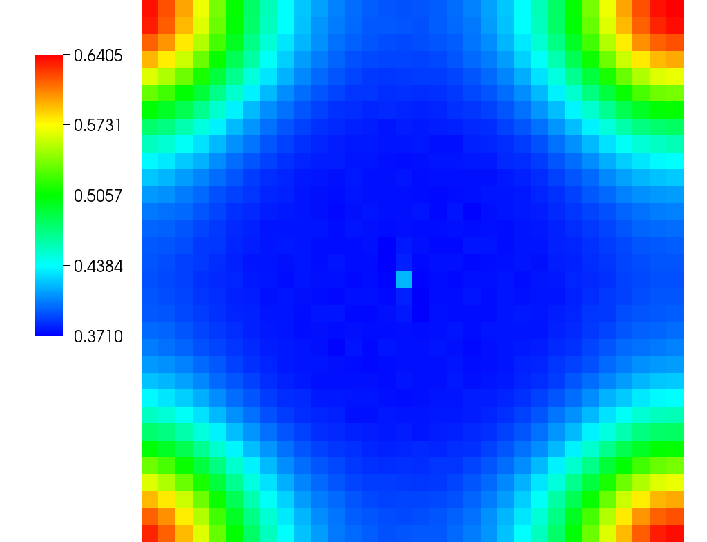
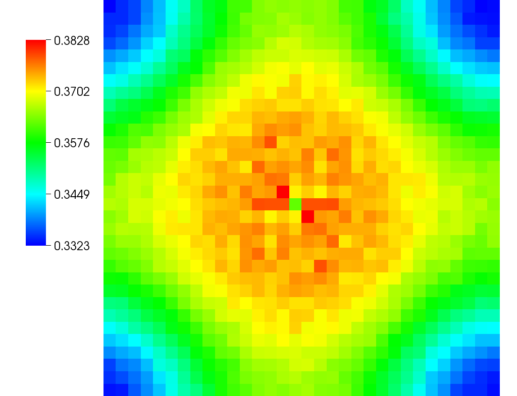
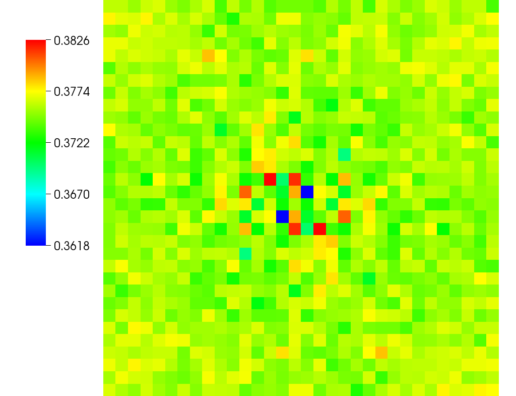
Figure 1: Equilibrium static structure factor $S_{\rho}$ as a function of wavevector (zero being at the center of the figures) for the overdamped simulations with $\Delta t=0.1$ (left), $\Delta t=0.05$ (middle), and $\Delta t=0.025$ (right). The correct result, which is recovered in the limit $\Delta t\rightarrow 0$, is $S_{\rho}=0.375$. The artifacts decrease by roughly a factor of 8 as the time step is reduced in half.

IV.2 Deterministic Lid-Driven Cavity Convergence Test

In this section, we simulate a smooth test problem and empirically confirm deterministic second-order accuracy of Algorithms 1 and 2 even in the presence of boundary conditions, inertial effects, and gravity, as well as nonconstant density, mass diffusion coefficient, and viscosity. The problem is a deterministic lid-driven cavity flow, following previous work by Boyce Griffith for incompressible constant-density and constant-viscosity flow NonProjection_Griffith .

We use CGS units (centimeters for length, seconds for time, grams for mass). We consider a square (two dimensions) or cubic (three dimensions) domain with side of length $L=1$ bounded on all sides by no-slip walls moving with a specified velocity. The bottom and top walls ($y$-direction) are no-slip walls moving in equal and opposite directions, setting up a circular flow pattern, while the remaining walls are stationary. The top wall has a specified velocity, in two dimensions,

$$u(x,t)=\begin{cases}\frac{1}{4}\left[1+\sin{(2\pi x-\frac{\pi}{2}})\right]\left[1+\sin{(2\pi t-\frac{\pi}{2}})\right],&t<1/2\\ \frac{1}{2}\left[1+\sin{(2\pi x-\frac{\pi}{2}})\right],&t\geq 1/2\end{cases}$$ (21)

and in three dimensions,

$$u(x,z,t)=w(x,z,t)=\begin{cases}\frac{1}{8}\left[1+\sin{(2\pi x-\frac{\pi}{2}})\right]\left[1+\sin{(2\pi z-\frac{\pi}{2}})\right]\left[1+\sin{(2\pi t-\frac{\pi}{2}})\right],&t<1/2\\ \frac{1}{4}\left[1+\sin{(2\pi x-\frac{\pi}{2}})\right]\left[1+\sin{(2\pi z-\frac{\pi}{2}})\right].&t\geq 1/2\end{cases}.$$ (22)

Note that the wall velocity tapers to zero at the corners in order to regularize the corner singularities NonProjection_Griffith ; similarly, the velocity smoothly increases with time to its final value in order to avoid potential loss of accuracy due to an impulsive start of the flow. The two liquids have pure-component densities $\bar{\rho}_{1}=2$ and $\bar{\rho}_{2}=1$. The initial conditions are $\boldsymbol{v}=0$ for velocity, and a Gaussian bump of higher density for the concentration, $c\left(\boldsymbol{r},t\right)=\exp\left(-75r^{2}\right)$, where $r$ is the distance to the center of the domain. The viscosity varies linearly as a function of concentration, such that $\eta=0.1$ when $c=0$ and $\eta=1$ when $c=1$. Similarly, the mass diffusion coefficient varies linearly as a function of concentration, such that $\chi=10^{-4}$ when $c=0$ and $\chi=10^{-3}$ when $c=1$. In order to confirm that second-order accuracy is preserved even in the limit of infinite Peclet number if BDS advection is employed, we also perform simulations with $\chi=0$. Figure 2 illustrates the initial and final (at time $t=2$) configurations of concentration and velocity in two dimensions.

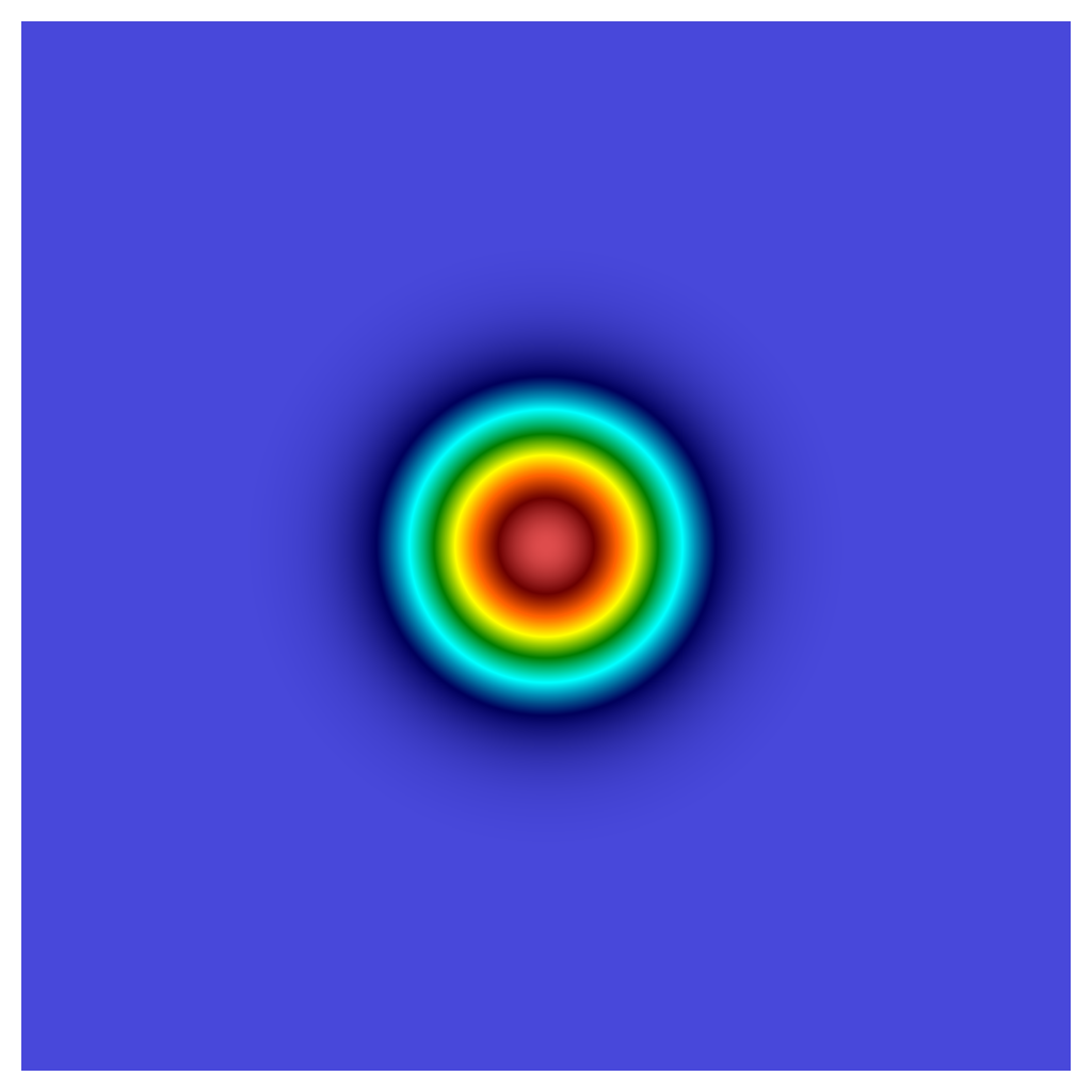
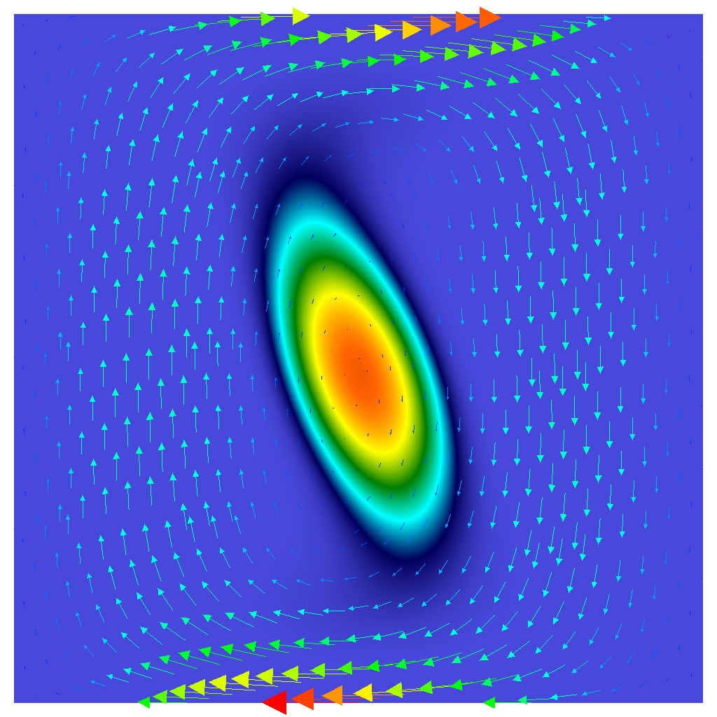
Figure 2: Initial ($t=0$) and final ($t=2$) concentration (scalar color field) and velocities (vector field) for the low Mach number lid-driven cavity test problem.

Recall that advection of the concentration can be treated using centered advection or the BDS advection scheme (see Section III.2.1). BDS advection can use either a bi-linear (trilinear in 3D) or a quadratic reconstruction (2D only), and can further be limited to avoid the appearance of spurious local extrema. Here we present convergence results for the following test problems:

• Test 1: Centered advection, nonzero $\chi$

• Test 2: Unlimited bilinear BDS advection, nonzero $\chi$

• Test 3: Unlimited quadratic BDS advection, nonzero $\chi$

• Test 4: Unlimited bilinear BDS advection, $\chi=0$.

We perform Tests 1-4 using both the inertial Algorithm 1 and the overdamped Algorithm 2. The Reynolds number in this test is of order unity and there is only a small difference in the results for the inertial and overdamped equations. Recall that concentration is the only independent variable in the overdamped equations.

In two dimensions, we discretize the problem on a grid of $64^{2}$, $128^{2}$, $256^{2}$ or $512^{2}$ grid cells. The time step size for the coarsest simulation is $\Delta t=5\times 10^{-3}$ and is reduced by a factor of 2 as the resolution increases by a factor of 2. This corresponds to an advective Courant number of $v_{\text{max}}\Delta t/\Delta x\sim 0.3$ for each simulation. The diffusive Courant number is $\chi\Delta t/\Delta x^{2}\sim 0.16$ (recall that the stability limit is $1/4=0.25$ in two dimensions) for the finest simulation, reducing by a factor of 2 with each successive grid coarsening. We simulate the flow and compute error norms at time $t=2$. In table 2 we present estimates of the order of convergence in the $L_{\infty}$ (max) norm for the velocity components and concentration for the inertial equations. We see clear second-order pointwise convergence, without any artifacts near the boundaries. Similar results are obtained for the concentration in the overdamped limit, as shown in table 3.

Table 2: Convergence of errors in the $L_{\infty}$ norm for a two-dimensional inertial low Mach lid-driven cavity problem as the grid is refined in space and time, for the components of the velocity $\boldsymbol{v}=\left(u,v\right)$ and concentration $c$. Order of convergence is estimated from the error ratio between two successive refinements.

refinement		64-128	Order	128-256	Order	256-512
Test 1:	$u$	1.93e-03	1.91	5.12e-04	1.96	1.32e-04
	$v$	8.69e-04	1.99	2.19e-04	2.00	5.49e-05
	$c$	3.02e-04	1.99	7.60e-04	2.00	1.90e-04
Test 2:	$u$	1.92e-03	1.91	5.11e-04	1.95	1.32e-04
	$v$	9.08e-04	1.96	2.34e-04	1.99	5.91e-05
	$c$	2.63e-03	1.72	7.99e-04	1.92	2.11e-04
Test 3:	$u$	1.92e-03	1.91	5.11e-04	1.95	1.32e-04
	$v$	8.62e-04	1.95	2.23e-04	1.98	5.64e-05
	$c$	1.95e-03	1.99	4.91e-04	2.00	1.23e-04
Test 4:	$u$	1.91e-03	1.92	5.06e-04	1.96	1.30e-04
	$v$	9.78e-04	2.01	2.43e-04	2.02	6.00e-05
	$c$	4.29e-03	1.90	1.15e-03	1.97	2.93e-04

Table 3: Convergence of errors in the $L_{\infty}$ norm for a two-dimensional overdamped low Mach lid-driven cavity problem as the grid is refined in space and time, for concentration $c$. Order of convergence is estimated from the error ratio between two successive refinements.

refinement	64-128	Order	128-256	Order	256-512
Test 1:	3.57e-03	2.01	8.89e-04	2.00	2.22e-04
Test 2:	2.70e-03	1.78	7.87e-04	1.92	2.08e-04
Test 3:	1.95e-03	1.98	4.95e-04	1.89	1.34e-04
Test 4:	4.23e-03	1.93	1.11e-03	1.96	2.86e-04

In three dimensions, we discretize the problem on a grid of $32^{3}$, $64^{3}$, $128^{3}$ or $256^{3}$ grid cells. The time step size for the coarsest simulation is $\Delta t=1.25\times 10^{-2}$, which corresponds to an advective Courant number of $\sim 0.4$, and diffusive Courant number of $\sim 0.10$ (stability limit is $1/6\approx 0.17$) for the finest resolution simulation. We simulate the flow and compute error norms at time $t=1$. We limit our study here to inertial flow and only perform Tests 1 and 2 (note that there is presently no available unlimited quadratic BDS advection scheme in three dimensions, so test 3 cannot be performed). We also try a higher-order one-sided difference for the tangential velocity at the no-slip boundaries, which does not affect the asymptotic rate of convergence, but it can significantly reduce the magnitude of the errors, and enables us to reach the asymptotic regime for smaller grid sizes NonProjection_Griffith . The numerical convergence results shown in table 4 demonstrate the second-order deterministic accuracy of our method in three dimensions.

Table 4: Convergence of errors in the $L_{\infty}$ norm for a three-dimensional inertial low Mach lid-driven cavity problem as the grid is refined in space and time, for the components of the velocity $\boldsymbol{v}=\left(u,v,w\right)$ and concentration $c$. Order of convergence is estimated from the error ratio between two successive refinements.

		32-64	Rate	64-128	Rate	128-256
Test 1:	$u$	7.66e-03	1.75	2.27e-03	1.88	6.16e-04
	$v$	3.12e-03	1.96	8.02e-04	1.99	2.02e-04
	$w$	7.66e-03	1.75	2.27e-03	1.88	6.16e-04
	$c$	1.22e-02	2.00	3.06e-03	2.00	7.64e-04
Test 1:	$u$	2.30e-03	1.97	5.88e-04	2.02	1.45e-04
with higher-order	$v$	9.01e-04	2.23	1.92e-04	1.99	4.82e-05
boundary stencil	$w$	2.30e-03	1.97	5.88e-04	2.02	1.45e-04
	$c$	1.21e-02	1.99	3.05e-03	2.00	7.62e-04
Test 2:	$u$	7.67e-03	1.75	2.28e-03	1.89	6.16e-04
	$v$	3.11e-03	1.96	8.01e-04	1.99	2.02e-04
	$w$	7.67e-03	1.75	2.28e-03	1.89	6.16e-04
	$c$	9.79e-03	1.91	2.61e-03	1.97	6.68e-04
Test 2:	$u$	2.30e-03	1.96	5.89e-04	2.01	1.46e-04
with higher-order	$v$	8.90e-04	2.21	1.92e-04	1.99	4.82e-05
boundary stencil	$w$	2.30e-03	1.96	5.89e-04	2.01	1.46e-04
	$c$	9.70e-03	1.91	2.59e-03	1.96	6.67e-04

IV.3 Deterministic Sharp Interface Limit

In this section we verify the ability of the BDS advection scheme to advect concentration and density without creating spurious oscillations or instabilities, even in the absence of mass diffusion, $\chi=0$, and in the presence of sharp interfaces. The problem setup is similar to the inertial lid-driven cavity test presented above, with the following differences. First, the gravity is larger, $\boldsymbol{g}=(0,-5)$, so that the higher density region falls downward a significant distance. Secondly, the initial conditions are a constant background of $c=0$ with a square region covering the central 25% of the domain initialized to $c=1$ (see the left panel of Figure 3). The correct solution of the equations must remain a binary field, $c=1$ inside the advected square curve, and $c=0$ elsewhere. In this test we employ limited quadratic BDS, and use a grid of $256^{2}$ grid cells and a fixed time step size $\Delta t=2.5\times 10^{-3}$, corresponding to an advective CFL number of $\sim 0.6$. In Figure 3, we show the concentration at several points in time, observing very little smearing of the interface, even as the deformed bubble passes near the bottom boundary.

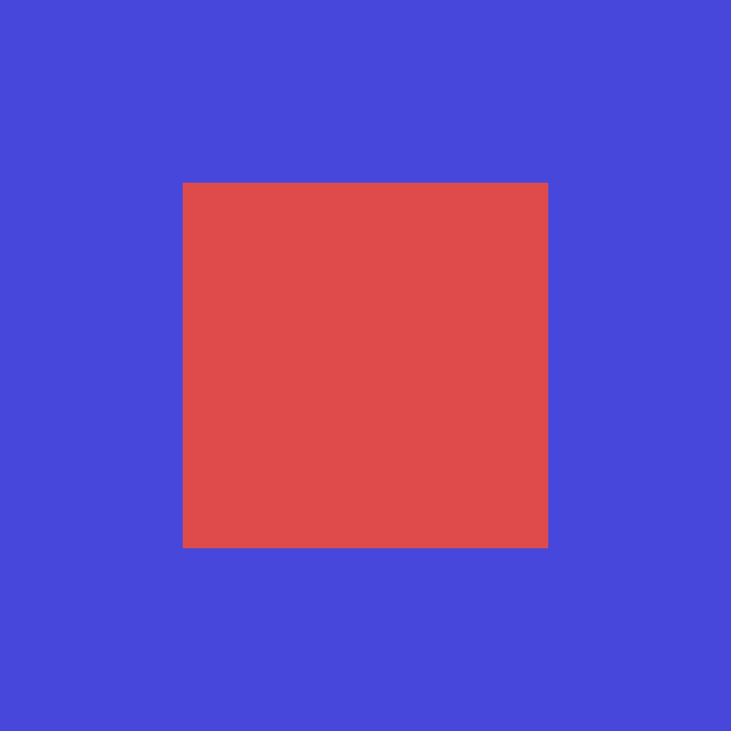
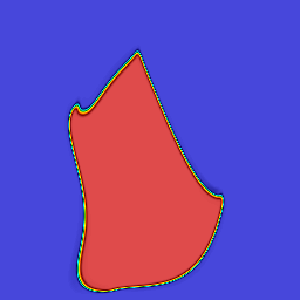
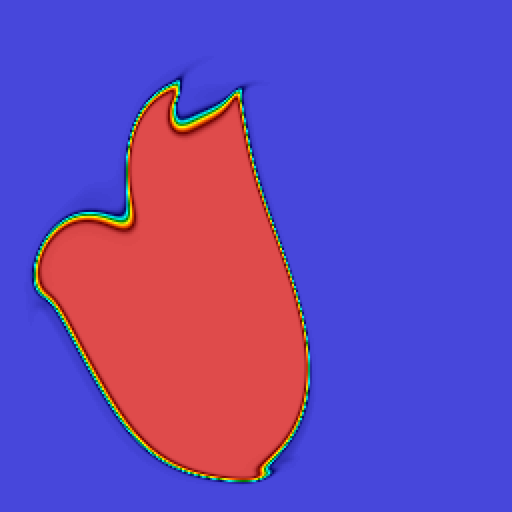
Figure 3: Advection of a square bubble in a lid-driven cavity flow, using the limited quadratic BDS scheme. Concentration is shown as a color plot at times $t=0,2,4$.

IV.4 Deterministic Kelvin-Helmoltz Instability

We simulate the development of a Kelvin-Helmholtz instability in three dimensions in order to demonstrate the robustness of our inertial time-advancement scheme in a deterministic setting. Our simulation uses $256\times 128\times 256$ computational cells with grid spacing $\Delta x=1/256$. We use periodic boundary conditions in the $x$ and $z$ directions, a no-slip conditions on the $y$ boundaries, with prescribed velocity $\boldsymbol{v}\left(x,y=0,z\right)=0$ on the bottom boundary and $\boldsymbol{v}\left(x,y=0.5,z\right)=(1,0,0)$ on the top boundary. We use an adaptive time step size $\Delta t$ adjusted to maintain a maximum advective CFL number $v_{max}\Delta t/\Delta x\leq 0.9$. The binary fluid mixture has a 10:1 density contrast with $\bar{\rho}_{1}=10$ and $\bar{\rho}_{2}=1$. Viscosity varies linearly with concentration, such that $\eta=10^{-4}$ for $c=0$ and $\eta=10^{-3}$ for $c=1$. The mass diffusion coefficient is fixed at $\chi=10^{-6}$, which makes the diffusive CFL number $\chi\Delta t/\Delta x^{2}\sim 10^{-4}$, making it necessary to use BDS advection in order to avoid instabilities due to sharp gradients at the interface. We employ the bilinear BDS advection scheme BDS with limiting in order to preserve strict monotonicity and maintain concentration within the bounds $0\leq c\leq 1$.

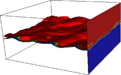
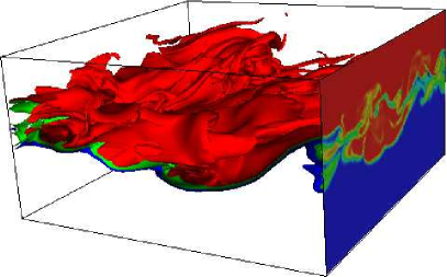
Figure 4: The development of a Kelvin-Helmholtz instability as a lighter less-viscous fluid streams over a ten times denser and more viscous fluid. Contour surfaces of the density, ranging from $\rho=1$ (red) to $\rho=10$ (blue), are shown at times $t=1.72,\,3.16,\,4.53$, and $5.85$s.

The initial condition is $c=1$ in the lower-half of the domain, and $c=0$ in the upper-half of the domain, so that light fluid sits on top of heavy fluid with a discontinuity in the concentration and velocity at the interface. The initial momentum is set to $\rho\boldsymbol{v}=(1,0,0)$ in the upper-half of the domain and $\rho\boldsymbol{v}=0$ in the lower-half of the domain. Gravity has a magnitude of $g=0.1$ acting in the downward $y$-direction. In order to set off the instability, in a row of cells at the centerline, $c$ is initialized to a random value between 0 and 1. The subsequent temporal evolution of the density (which is related to concentration via the EOS) is shown in Fig. 4, showing the development of the instability with no visible numerical artifacts. We also observe uniformly robust convergence of the GMRES Stokes solver throughout the simulation.

V Giant Concentration Fluctuations

Advection of concentration by thermal velocity fluctuations in the presence of large concentration gradients leads to the appearance of giant fluctuations of concentration, as has been studied theoretically and experimentally for more than a decade GiantFluctuations_Nature ; GiantFluctuations_Theory ; GiantFluctuations_Cannell ; FractalDiffusion_Microgravity ; GiantFluctuations_Summary . In this Section, we use our algorithms to simulate experiments measuring the temporal evolution of giant concentration fluctuations during free diffusive mixing in a binary liquid mixture. In Ref. GiantFluctuations_Cannell , Croccolo et al. report experimental measurements of the temporal evolution of the time-correlation functions of concentration fluctuations during the diffusive mixing of water and glycerol. In the experiments, a solution of glycerol in water with mass fraction of $c=0.39$ is carefully injected in the bottom half of the experimental domain, under the $c=0$ pure water in the top half. The two fluids slowly mix over the course of many hours while a series of measurements of the concentration fluctuations are performed.

In the experiments, quantitative shadowgraphy is used to observe and measure the strength of the fluctuations in the concentration via the change in the index of refraction. The observed light intensity, once corrected for the optical transfer function of the equipment, is proportional to the intensity of the fluctuations in the concentration averaged along the vertical (gradient) direction,

$$c_{\perp}(x,z;\,t)=H^{-1}\int_{y=0}^{H}c(x,y,z;\,t)dy,$$

where $H$ is the thickness of the sample in the vertical direction. The quantity of interest is the correlation function of the Fourier coefficients $\widehat{\delta c}_{\perp}\left(k_{x},k_{z};\,t\right)$ of $c_{\perp}(x,z;\,t)$,

$$C\left(\tau;\,t,k\right)=\left\langle\left(\widehat{\delta c}_{\perp}\left(k_{x},k_{z};\,t+\tau\right)\right)\left(\widehat{\delta c}_{\perp}\left(k_{x},k_{z};\,t\right)\right)^{\star}\right\rangle,$$

where $k=\sqrt{k_{x}^{2}+k_{z}^{2}}$ is the wavenumber (in our two dimensional simulations $k_{z}=0$), $\tau$ is a delay time, and $t$ is the elapsed time since the beginning of the experiment. In principle, the averaging above is an ensemble average but in the experimental analysis, and also in our processing of the simulation results, a time averaging over a specified time window $T$ is performed in lieu of ensemble averaging. This approximation is justified because the system is ergodic and the evolution of the deterministic (background) state occurs via slow diffusive mixing of the water and glycerol solutions, and thus happens on a much longer time scale (hours) than the time delays of interest (a few seconds).

The Fourier transform (in time) of $C\left(\tau\right)$ is called the dynamic structure factor. The equal-time correlation function

$$S\left(k;\,t\right)=C\left(\tau=0;\,t,k\right)$$

is the static structure factor, and is more difficult to measure in experiments GiantFluctuations_Cannell . For this reason, the experimental results are presented in the form of normalized time-correlation functions,

$$\widetilde{C}\left(\tau;\,t,k\right)=\frac{C\left(\tau;\,t,k\right)}{S\left(k;\,t\right)}.$$

The wavenumbers observed in the experiment and simulation are $k=\kappa\cdot 2\pi/L$, where $\kappa$ is an integer and $L$ is the horizontal extent of the observation window or the simulation box size. When evaluating the theory, we account for errors in the discrete approximation to the continuum Laplacian by using the effective wavenumber

$$k_{\perp}=k_{x}\frac{\sin\left(k_{x}\Delta x/2\right)}{\left(k_{x}\Delta x/2\right)}$$ (23)

instead of the actual discrete wavenumber $k_{x}$ LLNS_Staggered .

The confinement in the vertical direction is expected to play a small role because of the large thickness (2cm) of the sample, and a simple quasi-periodic (bulk) approximation can be used. Approximate theoretical analysis FluctHydroNonEq_Book suggests that at steady state the dominant nonequilibrium contribution to the static structure factor,

$$S\left(k;t\right)=\frac{k_{B}T}{\left(\eta\chi k^{4}-\rho\beta gh\right)}\,h^{2},$$ (24)

exhibits a $k^{-4}$ power-law decay at large wavenumbers, and a plateau to $k_{B}T\,h/\left(\rho\beta g\right)$ for wavenumbers smaller than a rollover $k_{c}^{4}=\rho\beta gh/\left(\eta\chi\right)$ due to the influence of gravity (buoyancy). Here $h\left(t\right)=d\bar{c}(y;t)/dy$ is the deterministic (background) concentration gradient, which decays slowly with time due to the continued mixing of the water and glycerol solutions.

An overdamped approximation suggests that the time correlations decay exponentially, $\widetilde{C}\left(\tau;\,t,k\right)=\exp\left(-\tau/\tau_{k}\right)$, with a relaxation time or decay time

$$\tau_{k}^{-1}=\chi k^{2}\left[1+\frac{\rho\beta gh}{\eta\chi k^{4}}\right],$$ (25)

that has a minimum at $k=k_{c}$ with value $\tau_{\text{min}}^{-1}=2\chi k_{c}^{2}\sim\sqrt{hg}$. For wavenumbers $k<k_{c}$ the relaxation time becomes smaller and can in fact become very small at the smallest wavenumbers, requiring small time step sizes in the simulations to resolve the dynamics and ensure stability of the temporal integrators. In the presence of gravity, at small wavenumbers the separation of time scales used to justify the overdamped limit fails and the fluid inertia has to be taken into account MultiscaleIntegrators . This changes the prediction for the time correlation function to be a sum of two exponentials with relaxation times,

$$\tau_{1/2}^{-1}=\frac{1}{2}\left(\nu+\chi\right)k^{2}\pm\frac{1}{2}\,\sqrt{k^{4}\left(\nu-\chi\right)^{2}-4\beta gh},$$ (26)

where $\nu=\eta/\rho$. This expression becomes complex-valued for

$$k\lesssim k_{p}=\left(\frac{4\beta gh}{\nu^{2}}\right)^{\frac{1}{4}}=\left(4\frac{\chi}{\nu}\right)^{\frac{1}{4}}k_{c},$$

indicating the appearance of propagative rather than diffusive modes for small wavenumbers, closely related to the more familiar gravity waves. While experimental measurements over wavenumbers $k\lesssim k_{p}$ are not reported by Croccolo et al GiantFluctuations_Cannell , their experimental data does contain several wavenumbers in that range. We report here simulation results for propagative concentration modes at small wavenumbers. To our knowledge, experimental observation of propagative modes has only been reported for temperature fluctuations TemperatureGradient_Cannell .

Because it is essentially impossible to analytically solve the linearized fluctuating equations in the presence of spatially-inhomogeneous density and transport cofficients and nontrivial boundary conditions, the existing theoretical analysis of the diffusive mixing process GiantFluctuations_Theory makes a quasi-periodic constant-coefficient and constant-gradient incompressible approximation FluctHydroNonEq_Book . This approximation, while sufficient for qualitative studies, is not appropriate for quantitative studies because the viscosity $\eta$ and mass diffusion coefficient $\chi$ vary by about a factor of three from the bottom to the top of the sample. In our simulations we account for the full dependence of density, viscosity and diffusion coefficient on concentration.

V.1 Simulation Parameters

For LFHD there is no difference between the two and three dimensional problems due to the symmetries of the problem FluctHydroNonEq_Book . Because very long simulations with a small time step size are required for this study, we perform two-dimensional simulations. Furthermore, in these simulations we do not include a stochastic flux in the concentration equation, i.e., we set $\boldsymbol{\Psi}=0$, so that all fluctuations in concentration arise from the coupling to the fluctuating velocity. With this approximation we do not need to model the chemical potential of the mixture and obtain $\mu_{c}$. This approximation is justified by the fact that it is known experimentally that the nonequilibrium fluctuations are much larger than the equilibrium ones for the conditions we consider GiantFluctuations_Cannell ; in fact, the fluctuations due to nonzero $\boldsymbol{\Psi}$ are smaller than solver or even roundoff tolerances in the simulations reported here.

We base our parameters on the experimental studies of diffusive mixing in a water-glycerol mixture, as reported by Croccolo et al. GiantFluctuations_Cannell . In the actual experiments the fluid sample is confined in a cylinder $2\,\mbox{cm}$ in diameter and $2\,\mbox{cm}$ thick in the vertical direction. In our simulations, the two-dimensional physical domain is $1.132\,\textrm{cm}\times 1.132\,\textrm{cm}$ discretized on a uniform $256\times 256$ two dimensional grid, with a thickness of $1\,\textrm{cm}$ along the $z$ direction. This large thickness makes the magnitude of the fluctuations very small since the cell volume $\Delta V$ contains a very large number of molecules, and puts us in the linearized regime MultiscaleIntegrators . The width of the domain $L=1.132\,\textrm{cm}$ is chosen to match the observation window in the experiments, and thus also match the discrete set of wavenumbers between the simulations and experiments. Earth gravity $g=-9.81\,\mbox{m}^{2}/\mbox{s}$ is applied in the negative $y$ (vertical) direction; for comparison we also perform a set of simulations without gravity. Periodic boundary conditions are applied in the $x$-direction and impenetrable no-slip walls are placed at the $y$ boundaries. The initial condition is $c=0.39$ in the bottom half of the domain and $c=0$ in the top half, with velocity initialized to zero. The temperature is kept constant at $300\,\mbox{K}$ throughout the domain. Centered advection is used to ensure fluctuation-dissipation balance over the whole range of wavenumbers represented on the grid.

A very good fit to the experimental equation of state (dependence of density on concentration at standard temperature and pressure) over the whole range of concentrations of interest is provided by the EOS (3) with the density of water set to $\bar{\rho}_{2}=1\,\textrm{g}/\textrm{cm}^{3}$ and the density of glycerol set to $\bar{\rho}_{1}=1.29\,\textrm{g}/\textrm{cm}^{3}$. Experimentally, the dependence of viscosity on glycerol mass fraction has been fit to an exponential function GiantFluctuations_Cannell , which we approximate with a rational function over the range of concentrations of interest WaterGlycerolViscosity ,

$$\eta(c)\approx\frac{1.009+1.1262\,c}{1-1.5326\,c}\cdot 10^{-2}\,\frac{\textrm{g}}{\textrm{cm}\,\mbox{s}}.$$ (27)

The diffusion coefficient dependence on the concentration has been studied experimentally, and we employ the fit proposed in Ref. WaterGlycerolDiffusion ,

$$\chi(c)=\frac{1.024-1.002\,c}{1+0.663\,c}\cdot 10^{-5}\,\frac{\textrm{cm}^{2}}{\mbox{s}},$$ (28)

which is in reasonable but not perfect agreeement with a Stokes-Einstein relation $\eta(c)\chi(c)=\mbox{const.}$ Note that the Schmidt number $S_{c}=\nu/\chi\sim 10^{3}$. In Ref. GiantFluctuations_Cannell , based on the experimental measurements and the approximate theoretical model, it is suggested that $\chi\approx 10^{-5}\,\textrm{cm}^{2}/\textrm{s}$ is constant over the range of concentrations present. For comparison, we also perform simulations in which we keep the diffusion coefficient independent of concentration, while still taking into account the concentration dependence of viscosity. It is worth noting that there is a notable disagreement between experimental measurements of $\chi(c)$ using different experimental techniques WaterGlycerolDiffusion and the true dependence is not known with the same accuracy as that of $\eta(c)$.

When gravity is present, we use the inertial Algorithm 1, with a rather small time step size $\Delta t=0.01375$s due to the fact that the smallest relaxation time measured is on the order of $0.1$s. For this time step size, the viscous CFL number is $\nu\Delta t/\Delta x^{2}\sim 10-30$, indicating that the viscous dynamics is resolved except at the wavenumbers comparable to the grid spacing. In the absence of gravity we use the overdamped Algorithm 2, which allows us to use a much larger time step size (on the diffusive time scale), $\Delta t=0.22$s, giving a diffusive CFL number on the order of $\chi\Delta t/\Delta x^{2}\lesssim 0.1$. Using larger time step sizes than this would require an implicit treatment of mass diffusion.

V.2 Results

Our simulations closely mimic the experiments of Croccolo et al GiantFluctuations_Cannell . We perform a long (stochastic) run of the diffusive mixing up to physical time $t=21,021$s, saving a snapshot and statistics every 21,840 time steps, which corresponds to 300 seconds of physical time. We then perform 8 short runs with different random seeds starting from the saved snapshots, and compute time correlation functions averaged over a short time interval. Note that in the experiments a similar procedure is used in which data is collected over short time intervals during a single long mixing process. Croccolo et al. report measurements at $t=600$s, $3060$s, $8160$s, and $14880$s. Table 5 lists the time intervals over which we collect statistics in the simulations, which match those in the experiments as well as possible. The time interval between successive snapshots used in the computation of the time correlation function is four time steps or 0.055s, which is four times smaller than the interval used in the experimental analysis. In the experiments averaging is performed over a range of wavenumbers in the $\left(k_{x},k_{z}\right)$ plane with similar magnitude. Since we perform two dimensional simulations we average over the 8 independent simulations; in the end the statistical errors are lower in the simulation results since experiment are subject to a large experimental noise not present in the simulations.

Starting Time	Total Time Steps	End Time
600.6 s	3328	$600+3328\Delta t=646.36$ s
3003 s	10784	3151.28 s
8108.1 s	4992	8176.74 s
15015 s	4768	15080.6 s

Table 5: Time intervals over which we average the dynamic correlation functions used to compute the relaxation times shown in Fig. 5.

V.2.1 Dynamic Structure Factors

In order to extract a relaxation time, we fit the numerical results for the normalized time-correlation function to an analytical formula. For the first four wavenumbers $k=\left(1,2,3,4\right)\cdot 2\pi/L$, clear oscillations (propagative modes) were observed, as illustrated in the left panel of Fig. 5. For these wavenumbers we used the fit

$$\widetilde{C}\left(t\right)=\exp\left(-\frac{t}{\tau}\right)\left(A\sin\left(2\pi\frac{t}{T}\right)+\cos\left(2\pi\frac{t}{T}\right)\right),$$ (29)

where the relaxation time $\tau$, the coefficient $A$ and the period of oscillation $T$ are the fitting parameters. For the remaining wavenumbers, we used a double-exponential decay for the fitting,

$$\widetilde{C}\left(t\right)=\alpha\exp\left(-\frac{t}{\tau_{1}}\right)+(1-\alpha)\exp\left(-\frac{t}{\tau_{2}}\right),$$ (30)

where $\alpha$, $\tau_{1}$ and $\tau_{2}$ are the fitting parameters. This leads to good fits for $k>k_{p}\sim 32\,\mbox{cm}^{-1}$; for a few transitional wavenumbers such as $k\sim 28\,\mbox{cm}^{-1}$ the fit is not as good, as illustrated in the left panel of Fig. 5. From the fit (30) we obtain the relaxation time $\tau$ as the point at which the amplitude decays by $\widetilde{C}\left(\tau\right)=1/e$.

A similar procedure was also used to obtain the relaxation time from the experimental data of Croccolo et al. GiantFluctuations_Cannell for all wavenumbers . The experimental data shows monotonically decaying correlation functions $\widetilde{C}\left(\tau;\,t,k\right)$ for all measured wavenumbers, not consistent with the oscillatory correlation function observed for the four smallest wavenumbers in our simulations MultiscaleIntegrators , see the left panel of Fig. 5. We believe that this mismatch is due to the way measurements for different wavenumbers of similar modulus are averaged in the experimental calculations. In our two-dimensional simulations, we do not perform any averaging over wavenumbers. We believe that the experimentally measured time correlation functions capture the real part of the decay times only and thus have the form of a sum of exponentials. Due to the lower time resolution and the fact that the static structure factor is not known, for the experimental data we used a single exponential fit and added an offset to account for the background noise,

$$C\left(t\right)=A\exp\left(-\frac{t}{\tau}\right)+B.$$

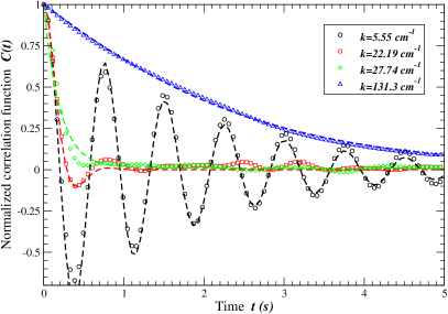
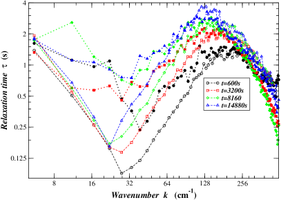
Figure 5: Dynamics of concentration fluctuations during free-diffusive mixing of water and glycerol. (Left) Numerical results for the time correlation functions for several selected wavenumbers about $8160$s from the beginning of the experiment. Symbols indicate results from the simulations and lines of the same color indicate the fit to (29) for the first ($k\approx 5.6\,\mbox{cm}^{-1}$) and fourth ($k\approx 22.2\,\mbox{cm}^{-1}$) wavenumbers, or to (30) for the remaining wavenumbers. Note that the statistical errors due to the finite averaging increase with time and the tails of the correlation functions are not reliably estimated. (Right) Relaxation or decay times as a function of wavenumber at several points in time. Empty symbols show results from computer simulations, and filled from experimental measurements GiantFluctuations_Cannell .

In the right panel of Fig. 5 we compare simulation and experimental results for the real part of the decay or relaxation time $\tau_{k}$, at several points in time measured from the beginning of the experiment. Good agreement is observed between the two with the same qualitative trends: A diffusive relaxation time $\tau_{k}^{-1}\approx\chi k^{2}$ for large wavenumbers, with a maximum at $k\approx k_{c}$, and then another minimum at $k\approx k_{p}$. Note that decay times are not reported by Croccolo et al GiantFluctuations_Cannell for wavenumbers $k\lesssim k_{p}$ since that work focuses on the effect of gravity for $k\lesssim k_{c}$. In our analysis of the experimental data we included all measured wavenumbers, including those for which propagative modes are observed. Here, the diffusion coefficient varies with concentration according to (28); very similar results for the relaxation times were obtained by keeping $\chi\approx 10^{-5}\,\textrm{cm}^{2}/\textrm{s}$ constant, as suggested by Croccolo et al GiantFluctuations_Cannell . This indicates that the dynamic correlations are not very sensitive to the concentration dependence $\chi(c)$. In future work we will perform a more careful comparison to experiments.

V.2.2 Static Structure Factors

Extracting the static structure factor from experimental measurements is complicated by several factors, including the presence of optical prefactors such as the transfer function of the instrument, and the appearance of additional contributions to the scattered light intensity such as shot noise, contributions due to giant temperature fluctuations TemperatureGradient_Cannell , and capillary waves GiantFluctuations_Interfaces ; GiantFluctuations_Capillary . We therefore study the evolution of the static structure factor using simulations only. In the left panel of Fig. 6 we show numerical results for the static structure factor $S\left(k;\,t\right)$ of the discrete concentration field averaged along the $y$-axes, at a series of times $t$ chosen to match those of the experimental measurements. Instead of ensemble averaging, here we performed a temporal average of the spectrum of the vertically-averaged concentration over a period of $300$s, ending at the time indicated in the legend of the figure. The characteristic $k^{-4}$ power law decay at large wavenumbers and the plateau at small wavenumbers predicted by (24) are clearly observed in Fig. 6, consistent with a value of $h$ decreasing with time. A quantitative difference is seen between the results for variable and constant diffusion coefficients, consistent with a different value of the imposed concentration gradient $h$ due to the somewhat different evolution of $\bar{c}(y,t)$.

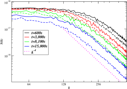
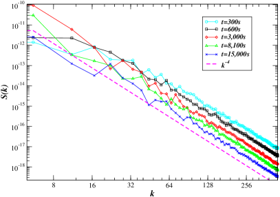
Figure 6: Evolution of the static structure factor during free-diffusive mixing of water and glycerol. (Left) With Earth gravity. Solid lines show results for simulations in which $\chi(c)$ depends on concentration according to (28), while dashed lines of the same color correspond to simulations in which $\chi\approx 10^{-5}\,\textrm{cm}^{2}/\textrm{s}$ is constant. Fluctuations at large wavenumbers follow a $k^{-4}$ power law but are damped by gravity at small wavenumbers. (Right) Without gravity; observe the large difference in the vertical axes showing “giant” fluctuations in the microgravity case. Note that these are results from a single simulation, mimicking a single experimeent, and therefore there are large statistical uncertainties at small wavenumbers (large decorrelation times).

In the right panel of Fig. 6 we show numerical results for the static structure factor that would be obtained had the experiment been performed in microgravity ($g=0$). In this case, we use the overdamped algorithm 2 since there is a persistent large separation of time scales between the slow concentration and fast velocity. We see clear development of a $k^{-4}$ power law as predicted by (24) for $g=0$. Note that here the concentration gradient is established instantaneously, in fact, it is the largest in the initial configuration and then decays on the diffusive time scale; this is different from simulations of the development of giant fluctuations in microgravity during the GRADFLEX experiment reported in MultiscaleIntegrators , in which the concentration gradient is slowly established on a diffusive scale. The results in Fig. 6 show that it takes some time for the giant fluctuations at smallest wavenumbers to develop; the diffusive relaxation time corresponding to the smallest wavenumber studied, $k_{\min}\approx 5\,\mbox{cm}^{-1}$ is $\tau_{\max}=\left(\chi k_{\min}^{2}\right)^{-1}\sim 4,000$s. After a time $\sim\left(\chi k^{2}\right)^{-1}$, the amplitude of the fluctuations $S(k)\sim k^{-4}h^{2}(t)$ decays slowly due to the diffusive mixing, and eventually the system will fully mix and reach thermodynamic equilibrium.

VI Conclusions

We have developed a low Mach number algorithm for diffusively-mixing mixtures of two liquids with potentially different density and transport coefficients. In the low Mach number setting, the incompressible constraint is replaced by a quasi-compressible constraint that dictates that stochastic and diffusive mass fluxes must create local expansion and contraction of the fluid to maintain a constant thermodynamic (base) pressure.

We employed a uniform-grid staggered-grid spatial discretization LLNS_Staggered . Following prior work in the incompressible simple-liquid case NonProjection_Griffith , we treated viscosity implicitly without splitting the pressure update, relying on a recently-developed variable-coefficient Stokes solver StokesKrylov for efficiency. This approach works well for any Reynolds number, including the viscous-dominated overdamped (zero Reynolds number) limit, even in the presence of nontrivial boundary conditions. Furthermore, by using a high-resolution BDS scheme BDS to advect the concentration we robustly handled the case of no mass diffusion (no dissipation in the concentration equation). In our spatial discretization we strictly preserved mass and momentum conservation, as well as the equation of state (EOS) constraint, by using a finite-volume (flux-based) discretization of advective fluxes in which fluxes are computing using extrapolated values of concentration and density that obey the EOS. Our temporal discretization used a predictor-corrector integrator that treats all terms except momentum diffusion (viscosity) explicitly MultiscaleIntegrators .

We empirically verified second-order spatio-temporal accuracy in the deterministic method. In the stochastic context, establishing the weak order of accuracy is nontrivial in the general low Mach number setting. For centered advection our temporal integration schemes can be shown to be second-order accurate for the special case of a Boussinesq constant-density (incompressible) approximation, or in the overdamped (inertia-free) limit. Existing stochastic analysis does not apply to the case of BDS advection because Godunov schemes do not fit a method-of-lines approach, but rather, employ a space-time construction of the fluxes. The presence of nontrivial density differences between the pure fluid components and nonzero mass diffusion coefficient, complicates the analysis even for centered advection, due to the presence of a nontrivial EOS constraint on the fluid dynamics. It is a challenge for future work to develop improved numerical analysis of our schemes in both the deterministic and the stochastic setting.

In future work, we will demonstrate how to extend the algorithms proposed here to multispecies mixtures of liquids using a generalization of the low Mach number constraint. The nontrivial multispecies formulation of the diffusive and stochastic mass fluxes has already been developed by some of us in the compressible setting MultispeciesCompressible .

It is also possible to include thermal effects in our formulation, by treating the temperature in a manner similar to the way we treated concentration here. Two key difficulties are constructing a spatial discretization that ensures preservation of an appropriately generalized EOS, as well as developing temporal integrators that can handle the moderate separation of time scales between the (typically) slower heat diffusion and (typically) faster momentum diffusion. In particular, it seems desirable to also treat temperature implicitly. Such implicit treatment of mass or heat diffusion is nontrivial because it would require solving coupled (via the EOS constraint) velocity-temperature or velocity-concentration linear systems, and requires further investigation.

In the staggered-grid based discretization developed here, we can only employ existing higher-order Godunov advection schemes for the cell-centered scalar fields such as concentration and density. It is a challenge for future work to develop comparable methods to handle advection of the staggered momentum field. This would enable simulations of large Reynolds number flows. It should be noted, however, that our unsplit approach is most advantageous at small Reynolds numbers.

A challenge for future work on low Mach number fluctuating hydrodynamics is to account for the effects of surface tension in mixtures of immiscible or partially miscible liquids. This can be most straightforwardly accomplished by using a diffuse-interface model, as some of us recently did in the compressible setting for a single-fluid multi-phase system CHN_Compressible . One of the key challenges is handling the fourth-order derivative term in the concentration equation in a way that ensures stability of the temporal integrator, as well as developing a consistent discretization of the Korteweg stresses on a staggered grid StagerredFluct_Inhomogeneous .

The semi-implicit temporal integrators we described here can deal well with a broad range of Reynolds or Schmidt numbers in the deterministic (smooth) setting. In the context of fluctuating hydrodynamics, however, all modes are thermally excited and treatment of viscosity based on a Crank-Nicolson method (implicit midpoint rule) are bound to fail for sufficiently large Schmidt numbers (or sufficiently low Reynolds numbers). In this work we solved this problem for the case of infinite Schmidt, zero Reynolds number flows by taking an overdamped limit of the original inertial equations before temporal discretization. It is a notable challenge for the future to develop uniformly accurate temporal integrators that work over a broad range of Reynolds or Schmidt numbers, including the asymptotic overdamped limit, in the presence of thermal fluctuations.

- (1) K. Balakrishnan, A. L. Garcia, A. Donev, and J. B. Bell. Fluctuating hydrodynamics of multispecies nonreactive mixtures. Phys. Rev. E, 89:013017, 2014.
- (2) A. K. Bhattacharjee, K. Balakrishnan, A. L. Garcia, J. B. Bell, and A. Donev. Fluctuating hydrodynamics of multispecies reactive mixtures. Submitted to J. Chem. Phys., ArXiv preprint 1503.07478, 2015.
- (3) Christophe Almarcha, Philip MJ Trevelyan, Patrick Grosfils, and Anne De Wit. Chemically driven hydrodynamic instabilities. Phys. Rev. Lett., 104(4):044501, 2010.
- (4) B. Z. Shang, N. K. Voulgarakis, and J.-W. Chu. Fluctuating hydrodynamics for multiscale simulation of inhomogeneous fluids: Mapping all-atom molecular dynamics to capillary waves. J. Chem. Phys., 135:044111, 2011.
- (5) A. Chaudhri, J. B. Bell, A. L. Garcia, and A. Donev. Modeling multiphase flow using fluctuating hydrodynamics. Phys. Rev. E, 90:033014, 2014.
- (6) A. Donev, A. L. Garcia, Anton de la Fuente, and J. B. Bell. Diffusive Transport by Thermal Velocity Fluctuations. Phys. Rev. Lett., 106(20):204501, 2011.
- (7) A. Vailati, R. Cerbino, S. Mazzoni, C. J. Takacs, D. S. Cannell, and M. Giglio. Fractal fronts of diffusion in microgravity. Nature Communications, 2:290, 2011.
- (8) J. M. O. De Zarate and J. V. Sengers. Hydrodynamic fluctuations in fluids and fluid mixtures. Elsevier Science Ltd, 2006.
- (9) B. Dünweg and A.J.C. Ladd. Lattice Boltzmann simulations of soft matter systems. Adv. Comp. Sim. for Soft Matter Sciences III, pages 89–166, 2009.
- (10) Sumesh P. T., Pagonabarraga I., and R. Adhikari. Lattice-boltzmann-langevin simulations of binary mixtures. Phys. Rev. E, 84:046709, 2011.
- (11) P. J. Atzberger. Stochastic Eulerian-Lagrangian Methods for Fluid-Structure Interactions with Thermal Fluctuations. J. Comp. Phys., 230:2821–2837, 2011.
- (12) F. Balboa Usabiaga, J. B. Bell, R. Delgado-Buscalioni, A. Donev, T. G. Fai, B. E. Griffith, and C. S. Peskin. Staggered Schemes for Fluctuating Hydrodynamics. SIAM J. Multiscale Modeling and Simulation, 10(4):1369–1408, 2012.
- (13) A. Donev, A. J. Nonaka, Y. Sun, T. G. Fai, A. L. Garcia, and J. B. Bell. Low Mach Number Fluctuating Hydrodynamics of Diffusively Mixing Fluids. Communications in Applied Mathematics and Computational Science, 9(1):47–105, 2014.
- (14) S. Klainerman and A. Majda. Compressible and incompressible fluids. Communications on Pure and Applied Mathematics, 35(5):629–651, 1982.
- (15) R. G. Rehm and H. R. Baum. The equations of motion for thermally driven buoyant flows. N. B. S. J. Res., 83:297–308, 1978.
- (16) A. Majda and J. Sethian. The derivation and numerical solution of the equations for zero Mach number combustion. Combustion science and technology, 42(3):185–205, 1985.
- (17) J. Lowengrub and L. Truskinovsky. Quasi-incompressible Cahn-Hilliard fluids and topological transitions. Proceedings of the Royal Society of London A, 454(1978):2617, 1998.
- (18) R.B. Pember, L.H. Howell, J.B. Bell, P. Colella, W.Y. Crutchfield, W.A. Fiveland, and J.P. Jessee. An adaptive projection method for unsteady, low-Mach number combustion. Combustion Science and Technology, 140(1-6):123–168, 1998.
- (19) T. Schneider, N. Botta, KJ Geratz, and R. Klein. Extension of finite volume compressible flow solvers to multi-dimensional, variable density zero Mach number flows. J. Comp. Phys., 155(2):248–286, 1999.
- (20) M. S. Day and J. B. Bell. Numerical simulation of laminar reacting flows with complex chemistry. Combustion Theory and Modelling, 4(4):535–556, 2000.
- (21) F. Nicoud. Conservative high-order finite-difference schemes for low-Mach number flows. J. Comp. Phys., 158(1):71–97, 2000.
- (22) B. Muller. Low-Mach-number asymptotics of the Navier-Stokes equations. Journal of Engineering Mathematics, 34(1):97–109, 1998.
- (23) S. Delong, Y. Sun, B. E. Griffith, E. Vanden-Eijnden, and A. Donev. Multiscale temporal integrators for fluctuating hydrodynamics. Phys. Rev. E, 90:063312, 2014.
- (24) J. B. Bell, P. Colella, and H. M. Glaz. A second order projection method for the incompressible Navier-Stokes equations. J. Comp. Phys., 85(2):257–283, 1989.
- (25) J. B. Bell, C. N. Dawson, and G. R. Shubin. An unsplit, higher order Godunov method for scalar conservation laws in multiple dimensions. J. Comput. Phys., 74:1–24, 1988.
- (26) Sandra May, Andrew Nonaka, Ann Almgren, and John Bell. An unsplit, higher-order godunov method using quadratic reconstruction for advection in two dimensions. Communications in Applied Mathematics and Computational Science, 6(1):27–61, 2011.
- (27) Andy Nonaka, S May, Ann S Almgren, and John B Bell. A three-dimensional, unsplit godunov method for scalar conservation laws. SIAM Journal on Scientific Computing, 33(4):2039–2062, 2011.
- (28) M. Cai, A. J. Nonaka, J. B. Bell, B. E. Griffith, and A. Donev. Efficient Variable-Coefficient Finite-Volume Stokes Solvers. Comm. in Comp. Phys. (CiCP), 16(5):1263–1297, 2014.
- (29) A. J. Chorin. Numerical Solution of the Navier-Stokes Equations. J. Math. Comp., 22:745–762, 1968.
- (30) A. S. Almgren, J. B. Bell, P. Colella, L. H. Howell, and M. L. Welcome. A conservative adaptive projection method for the variable density incompressible Navier-Stokes equations. J. Comput. Phys., 142:1–46, May 1998.
- (31) J. B. Bell, M. S. Day, C. A. Rendleman, S. E. Woosley, and M. A. Zingale. Adaptive low Mach number simulations of nuclear flame microphysics. J. Comp. Phys., 195(2):677–694, 2004.
- (32) A.S. Almgren, J.B. Bell, C.A. Rendleman, and M. Zingale. Low Mach number modeling of type Ia supernovae. I. Hydrodynamics. The Astrophysical Journal, 637(2):922, 2008.
- (33) S.Y. Kadioglu, R. Klein, and M.L. Minion. A fourth-order auxiliary variable projection method for zero-Mach number gas dynamics. Journal of Computational Physics, 227(3):2012–2043, 2008.
- (34) W. E and J.G. Liu. Gauge method for viscous incompressible flows. Commun. Math. Sci., 1(2):317–332, 2003.
- (35) David L Brown, Ricardo Cortez, and Michael L Minion. Accurate projection methods for the incompressible Navier-Stokes equations. Journal of Computational Physics, 168(2):464–499, 2001.
- (36) S. Delong, B. E. Griffith, E. Vanden-Eijnden, and A. Donev. Temporal Integrators for Fluctuating Hydrodynamics. Phys. Rev. E, 87(3):033302, 2013.
- (37) B.E. Griffith. An accurate and efficient method for the incompressible Navier-Stokes equations using the projection method as a preconditioner. J. Comp. Phys., 228(20):7565–7595, 2009.
- (38) A. Vailati and M. Giglio. Nonequilibrium fluctuations in time-dependent diffusion processes. Phys. Rev. E, 58(4):4361–4371, 1998.
- (39) F. Croccolo, D. Brogioli, A. Vailati, M. Giglio, and D. S. Cannell. Nondiffusive decay of gradient-driven fluctuations in a free-diffusion process. Phys. Rev. E, 76(4):041112, 2007.
- (40) A Vailati, R Cerbino, S Mazzoni, M Giglio, C J Takacs, and D S Cannell. Gradient-driven fluctuations in microgravity. Journal of physics. Condensed matter, 24(28):284134, 2012.
- (41) L.D. Landau and E.M. Lifshitz. Fluid Mechanics, volume 6 of Course of Theoretical Physics. Pergamon Press, Oxford, England, 1959.
- (42) H. C. Öttinger. Beyond equilibrium thermodynamics. Wiley Online Library, 2005.
- (43) P. Español, J.G. Anero, and I. Zúñiga. Microscopic derivation of discrete hydrodynamics. J. Chem. Phys., 131:244117, 2009.
- (44) A. Donev, T. G. Fai, and E. Vanden-Eijnden. A reversible mesoscopic model of diffusion in liquids: from giant fluctuations to Fick’s law. Journal of Statistical Mechanics: Theory and Experiment, 2014(4):P04004, 2014.
- (45) A. Donev and E. Vanden-Eijnden. Dynamic Density Functional Theory with hydrodynamic interactions and fluctuations. J. Chem. Phys., 140(23), 2014.
- (46) H. Grabert. Projection operator techniques in nonequilibrium statistical mechanics. Springer-Verlag, 1982.
- (47) M. Hütter and H.C. Öttinger. Fluctuation-dissipation theorem, kinetic stochastic integral and efficient simulations. J. Chem. Soc., Faraday Trans., 94(10):1403–1405, 1998.
- (48) G. Da Prato. Kolmogorov equations for stochastic PDEs. Birkhauser, 2004.
- (49) A. Donev, E. Vanden-Eijnden, A. L. Garcia, and J. B. Bell. On the Accuracy of Explicit Finite-Volume Schemes for Fluctuating Hydrodynamics. Communications in Applied Mathematics and Computational Science, 5(2):149–197, 2010.
- (50) A. Donev R. Cerbino, Y. Sun and A. Vailati. Dynamic scaling for the growth of non-equilibrium fluctuations during thermophoretic diffusion in microgravity. Submitted to Sci. Reps., ArXiv preprint 1502.03693, 2015.
- (51) Eric Yu Tau. A second-order projection method for the incompressible navier-stokes equations in arbitrary domains. Journal of Computational Physics, 115(1):147–152, 1994.
- (52) J.B. Bell, A. Garcia, and S. Williams. Computational fluctuating fluid dynamics. ESAIM: M2AN, 44(5):1085–1105, 2010.
- (53) A. Vailati and M. Giglio. Giant fluctuations in a free diffusion process. Nature, 390(6657):262–265, 1997.
- (54) C. J. Takacs, G. Nikolaenko, and D. S. Cannell. Dynamics of long-wavelength fluctuations in a fluid layer heated from above. Phys. Rev. Lett., 100(23):234502, 2008.
- (55) P. N. Shankar and M. Kumar. Experimental Determination of the Kinematic Viscosity of Glycerol-Water Mixtures. Proceedings of the Royal Society A: Mathematical, Physical and Engineering Sciences, 444(1922):573–581, 1994.
- (56) Gerardino D’Errico, Ornella Ortona, Fabio Capuano, and Vincenzo Vitagliano. Diffusion coefficients for the binary system glycerol+ water at 25 c. a velocity correlation study. Journal of Chemical & Engineering Data, 49(6):1665–1670, 2004.
- (57) P. Cicuta, A. Vailati, and M. Giglio. Equilibrium and nonequilibrium fluctuations at the interface between two fluid phases. Phys. Rev. E, 62(4):4920–4926, 2000.
- (58) P. Cicuta, A. Vailati, and M. Giglio. Capillary-to-bulk crossover of nonequilibrium fluctuations in the free diffusion of a near-critical binary liquid mixture. Applied Optics, 40(24):4140–4145, 2001.