Local Policies for Efficiently Patrolling
a Triangulated Region by a Robot Swarm

Abstract

We present and analyze methods for patrolling an environment with a distributed swarm of robots. Our approach uses a physical data structure – a distributed triangulation of the workspace. A large number of stationary “mapping” robots cover and triangulate the environment and a smaller number of mobile “patrolling” robots move amongst them. The focus of this work is to develop, analyze, implement and compare local patrolling policies. We desire strategies that achieve full coverage, but also produce good coverage frequency and visitation times. Policies that provide theoretical guarantees for these quantities have received some attention, but gaps have remained.

We present: 1) A summary of how to achieve coverage by building a triangulation of the workspace, and the ensuing properties. 2) A description of simple local policies (LRV, for Least Recently Visited and LFV, for Least Frequently Visited) for achieving coverage by the patrolling robots. 3) New analytical arguments why different versions of LRV may require worst-case exponential time between visits of triangles. 4) Analytical evidence that a local implementation of LFV on the edges of the dual graph is possible in our scenario, and immensely better in the worst case. 5) Experimental and simulation validation for the practical usefulness of these policies, showing that even a small number of weak robots with weak local information can greatly outperform a single, powerful robots with full information and computational capabilities.

I Introduction and Related Work

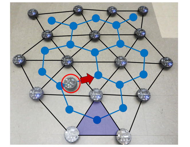
Figure 1: Triangulated network patrolling experiment with one patrolling robot (red circle). Blue lines indicate the dual graph of the triangulation. The blue triangle is the starting point for the patrol. The patrol policy computes the next adjacent triangle a patrolling robot should visit. It’s output is shown with the red arrow near the patrolling robot.

Large populations of robots are ideal for tasks where the robot must cover a large geographic area, such as search-and-rescue, exploration, mapping and surveillance. The robots can maintain coverage of the environment after the dispersion is complete. The size of the environment that can be covered is proportional to the population size, but large populations require that individual robot be quite simple, without expensive sensors or computation. In this paper, we focus on using a heterogeneous group of robots; with many small “mapping” robots that map the environment and build a communication network, and a smaller (but still numerous) number of more capable “patrolling” robots with the capability to respond to events. After deployment of the mapping robots, controlling the more powerful patrolling robots amounts to a coverage control problem: How should the navigating robots move in order to ensure small worst-case latency in patrolling all areas of the surveyed environment? Given the distributed nature of a swarm, this requires simple local strategies that do not involve complicated protocols or computations for coordinating the motion of the mobile components, while still achieving complete coverage, with small latency to surveyed locations.

In previous work [3, 8], we showed how complete coverage of an unknown region can be achieved by performing a structured exploration by a multi-robot system with bearing-only low-resolution sensors. The result is a triangulation of the workspace that can be exploited for further tasks. As described in [11] this supports a straightforward approach to patrolling: Each triangle can be considered a vertex in a dual graph, with adjacent triangles connected by dual edges. Thus, any route in the workspace that visits a sequence of triangles can be traced by a path in the dual graph. This can significantly reduce the computation on the patrolling robots – a simple policy that considers the current triangle and adjacent triangles will suffice. Given well-shaped triangles (which can be achieved by the robot platform described in this paper), a policy can produce a patrol with provable properties. Fig. 1 shows an example experiment.

What local policies should be used for patrolling the triangulated region? A natural choice for this task is Least Recently Visited (LRV), in which each triangle keeps track of the time elapsed since its last visit from a patrolling robot. The patrolling robot policy directs it to move to the adjacent triangle with the smallest such latency. This amounts to tracking the visit times of triangles, which are the vertices in the dual graph, the blue circles in Fig. 1. We show that this yields a policy that achieves complete coverage, and no obvious problems in practical experiments[11].

In this paper, we investigate the theoretical properties of patrolling policies. We present new results that show using LRV on dual vertices (i.e., LRV-v) can perform quite badly, by proving that the resulting coverage time can be exponential in the number $n$ of dual vertices. This is a new analytical result for our specific class of graphs that arise from planar triangulations, i.e., planar graphs of maximum degree three. We present alternate policies that share the simple local information requirements of LRV-v, while achieving latencies that are small even in the worst case. The policy Least Frequently Visited (LFV) that keeps track of the frequency of visits is such a candidate. Making this policy provably good requires a particular twist: instead of tracking visits to triangles, the dual vertices, we track the use of edges between triangles, the dual edges. We call these two new policies LFV-v and LFV-e respectively. We augment the physical data structure of our triangulated network to maintain these frequency counts, and show that this data can be stored and retrieved by patrolling robots with fixed-size communication messages. This leads to latencies that are well bounded, even in the worst case: for regions covered by $n$ triangles, the latency of LFV-e is not worse than $O(n\cdot d)$, where $d$ is the dual diameter of the region, i.e., the largest number of triangles that may have to be visited in a shortest path. For naturally shaped regions with bounded aspect ratio, this amounts to an upper bound of $O(n^{1.5})$. We present simulation results and hardware experiments with 19 robots that demonstrate the efficacy of our approach.

I-A Assumptions

We focus our attention on approaches applicable to small, low-cost devices with limited sensors and capabilities. In this work, we assume that robots do not have a map of the environment, nor the ability to localize themselves relative to the environment geometry, i.e. SLAM-style mapping is beyond the capabilities of our platform. Instead, we assume that the mapping robots can disperse and triangulate the environment; see [3] for an illustrative video, and [11] for a technical paper. We exclude solutions that use centralized control, as the communication and processing constraints do not allow these approaches to scale to large populations. We also do not assume that GPS localization or external communication infrastructure is available, which are limitations present in an unknown indoor environment. We assume that the communication range is much smaller than the size of the environment, so a multi-hop network is required for communication. Finally, we assume that the devices know the geometry of their local communications network. This local network geometry provides each robot with relative pose information about its neighbors.

I-B Related Work

Our results rely on the computational power of many small robots distributed throughout the environment, which support many basic algoritms. The patrolling robots use the mapping robot’s network for navigation, there are many references, we note that Batalin’s approach is similar to our own [2]. Our network is composed of triangles, which provide useful geometric properties. Approaches like those of Spears et al. [14] build a triangulated configuration using potential fields, but the network does not have a physical data structure, so the robots never recognize that they form triangles. Our approach allows us to use triangles as computational elements, which support practical distributed computations[11]. Geraerts [9] or Kallmann [10], use a triangulated environment for path planning, but require global information and localization. Our approach is fully distributed, using only local information and communications.

Optimizing the refresh frequency when patrolling a graph even by a single, powerful robot with full information amounts to finding a shortest roundtrip that visits all vertices – the well-known Traveling Salesman Problem (TSP), which is known to be NP-hard, even for full information and central control; see the book [1] for a comprehensive study of solution methods, and the book [4] for a recent overview of history and aspects of optimization. Simple approximation algorithms for the TSP that require a limited amount of computation do exist, for example, based on building a minimum spanning tree [6]; however, this still requires global information or communication, even with only local connections. Moreover, the problem for multiple robots amounts to the Vehicle Routing Problem (VRP), for which the additional task of finding a well-balanced distribution of vertices visited by the individual robots impedes performance guarantees for simple heuristics, such as doubling a spanning tree. This contributes to making the VRP very challenging in practical contexts. See the book by Toth and Vigo [15] for a comprehensive overview.

Motivated by using a swarm of weak robots, rather than powerful centralized methods, we favor approaches that require only local information, which can be maintained by the dual vertices. The most basic policy is to use a random walk for each robot. As discussed in detail by Cooper et al. [5], this has some obvious disadvantages in the worst case, and may even be of limited quality in the average case. Better approaches consider available information, such as the time elapsed since the last visit by a robot. This has been considered in the context of token passing in decentralized ad-hoc networks. As Malpani et al. [12] showed, the policy Least Recently Visited (LRV) ensures that finite refresh times can be guaranteed. However, one of the theoretical results by Cooper et al. [5] was to show that there are examples for which this policy may result in refresh times that are exponential in the size of the graph. More on this will be discussed in Section III, where we discuss LRV in the context of mobile robots.

II Model and Preliminaries

We have a system of $p$ mapping robots and $r$ patrolling robots, where $p\gg r$. The communication network is an undirected graph $G=(V,E)$. Each robot is modeled as a vertex, $u\in V$, where $V$ is the set of all robots and $E$ is the set of all robot-to-robot communication links. The neighbors of each vertex $u$ are the set of robots within line-of-sight communication range $r_{max}$ of robot $u$, denoted $N(u)=\{v\in V\ \mid\{u,v\}\in E\}$. We assume all network edges are also navigable paths. Robot $u$ sits at the origin of its local coordinate system, with the $\hat{x}$-axis aligned with its current heading. Robot $u$ can measure the relative pose of its neighbors in its reference frame. We model algorithm execution as a series of synchronous rounds. This simplifies analysis and is straightforward to implement in a physical system [13].

The mapping robots use our MATP triangulation algorithm [7, 3, 11], to explore and triangulate the environment. The exploration proceeds in a breadth-first fashion, leaving a triangulated network in its wake. Figure 2 shows an example triangulation of mapping robots. This primal graph $G_{P}=(V_{P},E_{P})$ consists of the $p$ triangulation robots, $V_{P}$, constructing the network, and the edges, $E_{P}$, forming the triangles. Pairs of triangulation robots with $\{v_{i},v_{j}\}\in E_{P}$ are able to communicate with each other, while any mobile robot $r$ inside a triangle formed by robots $v_{i}$, $v_{j}$, $v_{k}$ can communicate with all three of them. In turn, the set $V_{D}$ of triangles forms the vertices of a dual graph $G_{D}=(V_{D},E_{D})$, in which two vertices $\Delta_{i},\Delta_{j}\in V_{D}$ are connected by an edge if the triangles represented by $\Delta_{i}$ and $\Delta_{j}$ are adjacent. The triangulation algorithm guarantees that a dual edge $\{\Delta_{i},\Delta_{j}\}\in E_{D}$ corresponds to the primal edge $\{v_{i},v_{j}\}\in E_{P}$, where $v_{i}$ is the owner of triangle $\Delta_{i}$. This allows us to model computation on $\Delta_{i}$ and communication between $\Delta_{i}$ and $\Delta_{j}$ while the actual computation and communication is on $v_{i}$ and $\{v_{i},v_{j}\}\in E_{P}$. See [11] for details.

III Local Patrolling Policies

III-A Maintaining the Dual Graph

In the following section we focus on the dual graph, and consider the triangles as computational elements. However, computation in triangles actually occurs on the primal vertices (the robots). A crucial property is the following, established in [11].

Theorem 3.1

The owners of two adjacent triangles must also be connected.

Thus, a mobile robot in a triangle $\Delta_{i}$ can do status checks on neighboring triangles (i.e., neighbors of $\Delta_{i}$ in the dual graph) by asking the owner of $\Delta_{i}$ to query its neighbors in the primal graph.

In our new algorithms, it becomes important to consider local patrolling policies that are based on keeping track of dual edges instead of vertices. This makes it necessary to store and retrieve information on these dual edges. We can implement this by making the owner of a triangle also the owner of the dual edges to all adjacent triangles. It is important to observe that these owners of a dual edge are not the vertices of the corresponding primal edge. Implementing this on the stationary robots forming the primal graph can be based on the following result.

Theorem 3.2

Any dual edge has two owners that are connected in the primal graph.

For a proof, observe that any dual edge involves two triangles, whose owners are adjacent by Theorem 3.1. Moreover, it also follows that any primal vertex can only be the owner of a small number of dual edges, which bounds memory and communication usage. This allows us to model information stored in a distributed fashion on triangles and edges, and reason about communication via the dual graph.

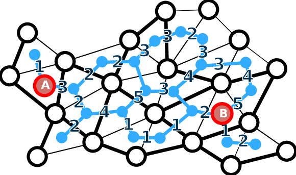
Figure 2: Notation for triangulation with a dual graph. Black circles:triangulation robots, red circles:patrolling robots, blue lines dual graph, black lines: primal graph edges that map to dual graph edges, thick black lines: subset of dual edges that indicate connections between owner vertices. The black numbers indicate the current data stored in each edge. For example, in LFV-e patrolling (Sec. III-B), this data would be the frequency of visits for that edge.

III-B Basic Policies

We consider a number of different local policies that allow patrolling all triangles of the environment. The objective is to minimize maximum latency, i.e., the longest refresh time ($RT$) between consecutive visits of the same triangle.

Our previous work described a local patrolling policy that moves each patrolling robot into the adjacent triangle with the largest refresh time. We refer to this policy as LRV-v, for least recently visited vertex). This design makes sense, as the objective is to keep refresh times small. While simple, this policy produces complete coverage [12].

The LRV policy has been studied in various contexts. Fig. 13 demonstrates that it exhibits relatively good behavior in practice. The experiment starts with one navigating robot; we add others as time proceeds. As we deploy more navigating robots, the maximum $RT_{t}({\Delta_{i}})$ decreases, as expected.

An alternative to considering the time since the last visit to a triangle is to keep track of the frequency of visiting. The rationale behind this is that an even distribution of visits should make the maximum latency close to the average. Thus, we obtain the policy LFV-v, for least frequently visited vertex.

Keeping track of visits to dual vertices (i.e., triangles) is natural, but not the only possible choice. Instead, we can track visits to dual edges, giving rise to the policies LRV-e and LFV-e. As it turns out, the crucial outcome of this paper is that both LRV-v and LFV-e have worst-case exponential latency, so they should be used only with care. While precise proofs on the worst-case behavior of LFV-v have yet to be established, we present evidence that it may also be bad. On the positive side, the worst-case behavior of LFV-e can be bounded, making it the unique policy of choice when trying to bound worst-case behavior.

III-C Worst-Case behavior of LRV-e and LRV-v

It is known that the worst-case behavior of LRV-e in arbitrary graphs can be exponential in the number of nodes in the graph, provided we allow a maximum degree of at least 4. That is, for every $n$ there exists a graph with $n$ vertices in which the largest refresh time for a node is $\exp(\Theta(n))$ [5]. Fig. 3 depicts one such graph (with vertices of degree 4), which filters a fixed percentage (1/3 to be precise) of all left-to-right paths that go past the diamond-like gadgets. If we connect $\Theta(n)$ such gadgets in series, we will require a total of $(3/2)^{\Theta(n)}$ paths, starting from the left for at least one of them to reach the rightmost point in the series.

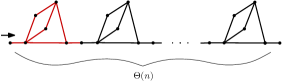
Figure 3: Graph with $n$ vertices with a chain of $\Theta(n)$ gadgets. A single gadget is colored in red for illustration purposes. Patrolling takes exponential time in the worst case [5].

Given that our scenario is based on visiting (dual) vertices, it is natural to consider the worst-case behavior of LRV-v for the special class of planar graphs of maximum degree 3 that can arise as duals of triangulations. Until now, this has been an open problem. Moreover, it also makes sense to consider the worst-case behavior of LRV-e for the same special graph class, which is not covered by the work of Cooper et al. [5].

Theorem 3.3

There are dual graphs of triangulations (in particular, planar graphs with $n$ vertices of maximum degree 3), in which LRV-v leads to a largest refresh time for a node that is exponential in $n$.

Proof.

Consider the graph $G_{D}$ in Fig. 4 colored in blue, which contains $\Theta(n)$ identical components connected in a chain. We prove the claimed exponential time bound by recursively calculating the time taken to complete one cycle in the transition diagram shown in Fig. 5.

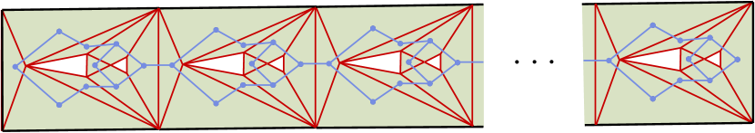
Figure 4: A polygonal region with holes triangulated (red lines) with the dual graph $G_{D}$ of the triangulation (blue lines).

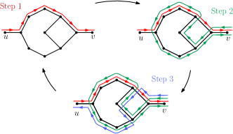
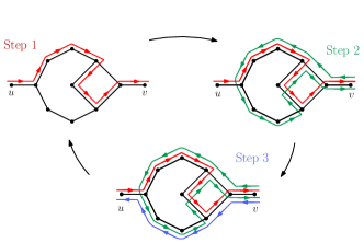
Figure 5: Two possible alternating paths for the LRV-v strategy on each component of the graph $G_{D}$.

We monitor the movement of a robot from this situation onwards. Let a robot take at least one unit of time to traverse an edge. Moreover, let $T_{n}$ denote the time taken to complete one cycle of $G_{D}$, i.e., the time taken by a robot to start from and return to the first vertex of the first component of $G_{D}$. From the possible paths illustrated in Fig. 5, we can observe that the vertex $u$ is visited only during the beginning and end of the cycle, while the vertex $v$ is visited twice in this cycle. It is not hard to check that the summation of visits to all edges in one component during one cycle is 26. Using this we can see a simple recursion as follows:

$$T_{n}\geq 26+2\cdot T_{n-1},\;T_{0}=0$$

Solving this equation, we get

$$T_{n}\geq 26\cdot(2^{n}-1)$$

Utilizing the fact that vertex $u$ of the first component is visited only at the beginning and end of a cycle in $G_{D}$, we see that it is visited after $T_{n}\geq 26\ast(2^{n}-1)$ units of time, which is exponential in the number $n$ of nodes of graph $G_{D}$, as claimed. ∎

As it turns out, the same negative result can be established for LRV-e, making both versions of LRV unsuitable for avoiding bad worst-case behavior.

Theorem 3.4

There are dual graphs of triangulations (in particular, planar graphs with $n$ vertices of maximum degree 3), in which LRV-e leads to a largest refresh time for a node that is quadratic in $n$.

Proof.

This proof follows the exact arguments as the proof of theorem 3.7 for the same graph $G_{D}$ represented in Fig. 11. As illustrated in Fig. 6, each of $G_{D}$’s components is traversed initially following the colored oriented paths from step 1 and further alternating the paths from step $2k$ and $2k+1$.

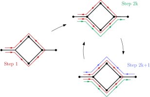
Figure 6: LRV-e strategy on each component of the graph $G_{D}$.

In other words, the first time a component is traversed, the path changes direction and goes back to the start. The rest of the times when the component is traversed, the direction does not change. Thus, in order to traverse the $i$th component in the chain, we need to traverse the first $i-1$ components in the chain. ∎

III-D Worst-Case behavior of LFV-v and LFV-e

In the following, we provide evidence that a small polynomial upper bound on the worst-case latency is unlikely for LFV-v. We start by showing some interesting properties of graphs explored under LFV-v. It would seem at first that paths in the graph must be in nonincreasing frequency. This is so as we always select the neighbor of lowest frequency. However, if all node’s neighbors have the same or higher frequency, then the destination node will have strictly larger frequency than the present neighbor (see Figs. 7 and 8).

Figure 7: A path being traversed from left to right with its frequency histogram below. Initially all nodes have frequency zero. Then half way through the path traversal nodes to left have frequency 1 and nodes to the right are still at zero.

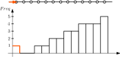
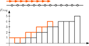
Figure 8: A path with a corresponding staircase pattern in the histogram.

Lastly we observe that it is possible to create dams or barriers by having a flower configuration in the path (see Fig. 9). We reach the center of the flower and then take the loops or petals, thus increasing the count of the center (see histogram on Fig. 9). Then the robot moves past the center node of the flower, which forms a barrier that impedes the robot from traversing from right to left past the center of the flower, until the count of the nodes to the right of the path has risen to match that of the barrier.

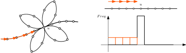
Figure 9: A path with a “flower” configuration which creates a barrier.

With these three basic configurations in hand, we can combine them to create a graph in which the starting node $s$ has $\delta(s)$ neighbors, $\delta-1$ of which lead via staircases with barriers to the last neighbor of $s$ which revisits $s$ (see Fig. 10). That is for each time we go from $s$ to one of the first $\delta-1$ neighbors we then climb a staircase up to the last common neighbor of $s$. Then from that neighbor we enter each staircase from the “high” side until stopped by a barrier, which makes us return to the neighbor of $s$, eventually revisiting $s$ from this last neighbor. This shows the following theorem.

Theorem 3.5

There exists a configuration for LFV-v in which some neighbors of the starting vertex have a frequency count of $k$, while the starting point has a frequency count of $k\,\delta$. Moreover, the value of $k$ can be as high as $\Theta(n/\delta)$.

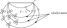
Figure 10: A configuration in which the frequency of the starting point $s$ is much larger than the majority of its neighbors.

This result provides some indication that the worst-case ratio between smallest and largest frequencey labels of vertices may be exponential, which would arise if we could construct an example in which $\Omega(\delta)$ linear ratios as in Theorem 3.5 between neighbors occur. From this it can be shown that at most $\delta^{d}$ steps are required to explore the graph, where $d$ and $\delta$ are the diameter and the maximum degree of the graph.

Theorem 3.6

The highest frequency node in a graph with unvisited nodes has frequency bounded by $\delta^{d}$.

Proof.

Consider a path from an unvisited node to the node with highest frequency. The path is of length at most the diameter $d$ of the graph. In each step the increase in frequency is at most a factor $\delta$ over the unvisited node hence the frequency of the most visited node is bounded by $\delta^{d}$. ∎

However, there is no known example of a dual of a triangulation graph displaying this worst-case behavior.

Theorem 3.7

There exist graphs with $n$ vertices of maximum degree 3, in which the largest refresh frequency for a node is $\Theta(n^{2}).$

Proof.

Consider the graph $G_{D}$ of Fig. 11 as described in its caption which consists of a chain of $\Theta(n)$ cycles of length 4 connected in series. As illustrated in Fig. 12, each component is traversed initially following the colored oriented paths from step 1 and further alternating the paths from step $2k$ and $2k+1$.

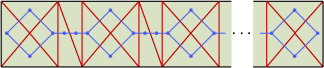
Figure 11: This figure depicts (1) a rectangular polygonal region in black lines (2) its triangulation $G_{P}$ in red lines and (3) the dual graph of the triangulation $G_{D}$ shown in blue lines.

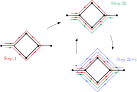
Figure 12: LFV-v strategy on each component of the graph $G_{D}$.

In other words, the first time a component is traversed, the path changes direction and goes back to the start. The rest of the times when the component is traversed, the direction does not change. Thus, in order to traverse the $i$th component in the chain, we need to revisit the first $i-1$ components in the chain. ∎

Thus, LFV-v may also display bad worst-case behavior. Fortunately, the following was proven by Cooper et al. [5] for the worst-case behavior of LFV-e.

Theorem 3.8

In a graph $G$ with at most $m$ edges and diameter $d$, the latency of each edge when carrying out LFV-e is at most $O(m\cdot d)$.

This allows us to establish a good upper bound on LFV-e in our setting.

Corollary 3.9

Let $G_{D}=(V_{D},E_{D})$ be the dual graph of a triangulation, with $|V_{D}|=n$ vertices and diameter $d$. Then the latency of each vertex when carrying out LFV-e is at most $O(n\cdot d)$.

Proof.

Since $G_{D}$ is planar, it follows that $n\in\Theta(m)$, where $m=|E_{D}|$ is the number of edges of $G_{D}$. Because patrolling an edge requires visiting both of its vertices, the claim follows from the upper bound of Theorem 3.8. ∎

We note that this bound can be tightened for regions with small aspect ratio, for which the diameter is bounded by the square root of the area.

Corollary 3.10

For regions with diameter $d\in O(\sqrt{n})$, the latency of each dual vertex when carrying out LFV-e is at most $O(n^{1.5})$.

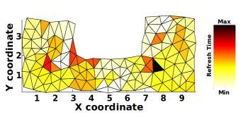
(a)

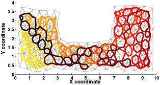
(b)

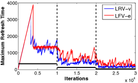
(c)

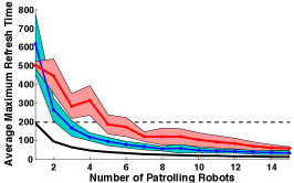
(d)

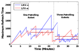
(e)

Figure 13: LABEL:sub@fig:MaxRefreshSimulationSetup Our simulated environment contains 193 triangles. The color of each triangle indicates the refresh time of the triangle. The black triangle in the middle of the triangulation has the maximum refresh time. LABEL:sub@fig:TracePatrol An example cyclic path from a single patrolling robot. The color of each path segment indicates the age, darkest color is the most recent path segment. This path produces a worst-case coverage with the tight bound on variance, as can be seen in the red trace of Fig. LABEL:sub@fig:MaxRefreshSimulationData. LABEL:sub@fig:MaxRefreshSimulationDataExample Maximum Refresh Time using LRV-v and LFV-e. Simulations start with one robot, and we put two and six additional robots at 10000 and 20000 iterations. Solid black lines indicate the lower bound of maximum refresh time of each patrolling robot, called baseline. LABEL:sub@fig:MaxRefreshSimulationData The trend of path length of each patrolling robot according to the number of patrolling robots. The black line shows the lower bound for a perfect set of disjoint patrolling cycles. The dotted line shows the best performance of a single robot. We ran the simulations using one to fifteen patrolling robots, $8\%$ of the number of triangles. LABEL:sub@fig:MaxRefreshRobotData Data from our patrolling experiment. Our experimental setup is shown in Fig 1. It consisted of 16 triangulation robots, and one or three patrolling robots. The experimental data is very similar to our simulation results.

IV Experimental Results

In order to validate and test our results, we performed a number of simulations, as well as experiments with a real-world platform. Fig. 14 shows the r-one platform, developed at Rice University.

Figure 14: Snapshot of the r-one robot used in the experiments.

An example simulation tun is shown in Fig 13a. Fig. 13c gives results from a real-world patrolling experiment with $1-3$ robots.

With one robot in the simulation, the LFV-e policy produces a closed path that resembles a Hamiltonian path, shown in Fig. 13b; as such a path is a theoretical lower bound, which is achievable only in exceptional cases, it is intuitively clear that we are getting excellent results. As we add more patrolling robots, the consolidated Hamiltonian-like path is perturbed and the variance of the maximum refresh time increases, shown in the red line (after 10K iterations) in Fig. 13c. Analyzing the paths of multiple robots show that there is some overall rebalancing in addition to finding new individual subtours. This corresponds to handling the two aspects of balancing loads and finding tours, which are both computationally hard in an offline setting. It can be seen that the LFV-e policy carries out more delicate operations, leading to a greate amount of initial perturbation. However, it is clear from the aggregated results shown in Fig. 13c that eventually, LFV-e yields superior results. Shown is the average maximum $RT_{\Delta_{i}}(t)$ for larger numbers of patrolling robots. The solid black line shows the lower bound for an optimal set of patrols. Assuming all of the patrolling robots are on their own Hamiltonian path, we can compute this lower bound by $\frac{|H(G)|}{r}$, where $|H(G)|$ is the length of a Hamiltonian cycle of the dual graph $G$ (the number of triangles), and $r$ is the number of patrolling robots. Despite of these differences between LRV-v and LFV-e, it is remarkable that both policies performed well, with a clearly evident linear speedup according to increasing number $r$ of robots. (Refer to the theoretically optimal lower bound mapped by the black hyperbola.)

Our hardware experimental setup is shown in Fig 1, and the data for a experiment is shown in Fig. 13e. The experiment started with one patrolling robot in the blue triangle. At 22 minutes into the experiment, we added two more robots, one in the blue triangle, and the other in the triangle to its left. The horizontal lines show the average refresh time in the last 10 minutes of patrolling. The LRV-v averages are 984 for one robot and 365 for three, and the LFV-e averages are 750 for one robot and 485 for three. Units are robot rounds. These data match our simulation results nicely. The experiment starts with one navigating robot; we add two more robots at 10k iterations, and then another 5 at 20k iterations. As we deploy more navigating robots, the maximum $RT_{\Delta_{i}}(t)$ decreases, seen in the red line. Note that here, too, LFV-e has the longest initialization before it discovers all of the triangles, the variance in the max refresh time is the smallest, once the patrolling routine has settled down.

V Conclusion

We have demonstrated how a combination of a weak stationary swarm with a set of mobile robots with limited capabilities can perform well for purposes of patrolling and surveillance of a region. The simple policy LRV (based on purely local information without any sophisticated communication between devices) allows complete coverage of the mapped area, but may lead to exponential refresh times for all portions in specific worst-case examples; the alternative policy LFV is of similar simplicity can protect against this worst-case behavior, provided it is applied to crossed edges of triangular subregions instead of the subregions themselves. In realistic simulations as well as real-world experiments, both policies perform quite well. Most remarkably, they display linear speedup for the visiting frequencies of the surveyed subregions, implying that even simple local policies on weak robots can vastly outperform single, powerful robots with full information and strong computational capabilities.

References

- [1] David L. Applegate, Robert E. Bixby, Vasek Chvátal, and William J. Cook. The Traveling Salesman Problem: A Computational Study. Princeton University Press, 2006.
- [2] Maxim Batalin and Gaurav S. Sukhatme. Using a sensor network for distributed Multi-Robot task allocation. In IEEE International Conference on Robotics and Automation, pages 158–164, New Orleans, Louisiana, April 2004.
- [3] Aaron Becker, Sándor P. Fekete, Alexander Kröller, Seoung Kyou Lee, James McLurkin, and Christiane Schmidt. Triangulating unknown environments using robot swarms. In Proc. 29th Annu. ACM Sympos. Comput. Geom., pages 345–346, 2013. Video available at http://imaginary.org/film/triangulating-unknown-environments-using-robot-swarms.
- [4] William J. Cook. In Pursuit of the Traveling Salesman: Mathematics at the Limits of Computation. Princeton University Press, 2012.
- [5] Colin Cooper, David Ilcinkas, Ralf Klasing, and Adrian Kosowski. Derandomizing random walks in undirected graphs using locally fair exploration strategies. Distributed Computing, 24(2):91–99, 2011.
- [6] Yehuda Elmaliach, Noa Agmon, and Gal A. Kaminka. Multi-robot area patrol under frequency constraints. Ann. Math. Artif. Intell., 57(3-4):293–320, 2009.
- [7] Sándor P. Fekete, Tom Kamphans, Alexander Kröller, J.S.B. Mitchell, and Christiane Schmidt. Exploring and triangulating a region by a swarm of robots. In Proc. APPROX 2011, volume 6845 of LNCS, pages 206–217. Springer, 2011.
- [8] Sándor P. Fekete, Seoung Kyou Lee, Alejandro López-Ortiz, Daniela Maftuleac, and James McLurkin. Patrolling a region with a structured swarm of robots with limited individual capabilities. In International Workshop on Robotic Sensor Networks (WRSN), 2014.
- [9] Roland Geraerts. Planning short paths with clearance using explicit corridors. In IEEE International Conference on Robotics and Automation (ICRA), pages 1997–2004. IEEE, 2010.
- [10] Marcelo Kallmann. Path planning in triangulations. In Proceedings of the IJCAI workshop on reasoning, representation, and learning in computer games, pages 49–54, 2005.
- [11] Seoung Kyou Lee, Aaron Becker, Sándor P. Fekete, Alexander Kröller, and James McLurkin. Exploration via structured triangulation by a multi-robot system with bearing-only low-resolution sensors. In IEEE International Conference on Robotics and Automation (ICRA), 2014. Available at http://arxiv.org/abs/1402.0400.
- [12] Navneet Malpani, Yu Chen, Nitin H. Vaidya, and Jennifer L. Welch. Distributed token circulation in mobile ad hoc networks. IEEE Trans. Mob. Comput., 4(2):154–165, 2005.
- [13] James McLurkin. Analysis and Implementation of Distributed Algorithms for Multi-Robot Systems. Ph.D. thesis, Massachusetts Institute of Technology, 2008.
- [14] W. M. Spears, D. F. Spears, J. C. Hamann, and R. Heil. Distributed, Physics-Based control of swarms of vehicles. Autonomous Robots, 17(2):137–162, 2004.
- [15] Paolo Toth and Daniele Vigo. The vehicle routing problem. Siam, 2001.