The Effect of Surface Brightness Dimming in the Selection of High-$z$ Galaxies

Abstract

Cosmological surface brightness dimming of the form $(1+z)^{-4}$ affects all sources. The strong dependence of surface brightness dimming on redshift $z$ suggests the presence of a selection bias when searching for high-redshift galaxies, i.e. we tend to detect only those galaxies with a high surface brightness (SB). However, unresolved knots of emission are not affected by SB dimming, thus providing a way to test the clumpiness of high-$z$ galaxies. Our strategy relies on the comparison of the total flux detected for the same source in surveys characterized by different depth. For all galaxies, deeper images permit the better investigation of low-SB features. Cosmological SB dimming makes these low-SB features hard to detect when going to higher and higher redshifts. We used the GOODS and HUDF Hubble Space Telescope legacy datasets to study the effect of SB dimming on low-SB features of high-redshift galaxies and compare it to the prediction for smooth sources. We selected a sample of Lyman-break galaxies at $z\sim 4$ (i.e. $B_{\rm 435}$-band dropouts) detected in all of the datasets and found no significant trend when comparing the total magnitudes measured from images with different depth. Through Monte Carlo simulations we derived the expected trend for galaxies with different SB profiles. The comparison to the data hints at a compact distribution for most of the rest-frame ultraviolet light emitted from high-$z$ galaxies.

1. Introduction

The surface brightness (SB) dimming derived by Tolman (1930, 1934) affects all cosmological sources. In particular, since for every extended source the surface brightness $I$ is no longer redshift-independent as in an Euclidean Universe, there is an additional term that should be taken into account. The contributions of time dilation, redshift, and curvature make high-$z$ galaxies progressively difficult to detect according to

$$I_{0}=\frac{I_{e}}{(1+z)^{4}}$$ (1)

where $I_{0}$ and $I_{e}$ are the observed and intrinsic surface brightnesses of the object, respectively. In particular, this effect is relevant for sources at $z\geq 4$ that dim by a factor greater than 600. The observational effect of cosmological dimming is a bias in the detection of very high-$z$ galaxies, i.e. we tend to detect only those galaxies with a high surface brightness. The dimming effect affects our understanding of the reionization phase as well, since the role of galaxies in this process and, in particular, the amount of ionizing radiation produced depends directly on the number of high-$z$ candidates detected in deep surveys.

The first studies on cosmological dimming and the consequent observational bias towards more compact objects at higher redshifts were conducted by Phillipps et al. (1990), but only up to redshift about 0.3. Later, Pascarelle et al. (1998) and Lanzetta et al. (2002) stated that a correction is needed in order to sample high and low-$z$ galaxies at the same SB threshold and that only the bright regions of galaxies are observable at high-$z$, since the faint ones cannot be detected against the background. A comprehensive discussion on Tolman dimming can be found in Disney & Lang (2012) who studied the surface brightness selection in the framework of the search for progenitors of low-$z$ galaxies. On the basis of Tolman dimming effect, they claim that, looking back in time, there should be different kind of objects at different epochs, in particular more compact objects at higher redshifts. Moreover, they claim the high-$z$ galaxy population, mostly hidden because of dimming effects, could be the source of the ionizing flux required to reionize the Universe . We will not discuss this aspect here. Our comprehensive study of the role of faint undetected galaxies in cosmic reionization is presented in Calvi et al. (2013).

In the last 20 years, the Hubble Space Telescope (HST) has enabled the astronomical community to study the morphology of Lyman Break Galaxies (LBGs) at different redshifts, from $z\sim 1.5$ up to $z\sim 7-8$, and all those objects were found to be compact (Giavalisco et al., 2004; Lotz et al., 2006; Oesch et al., 2010; Williams et al., 2014). Bouwens et al. (2004) found that the principal effect of depth in galaxy surveys is to add galaxies at fainter magnitudes, with an approximate $(1+z)^{-1}$ trend on the sizes. In particular, since galaxies at high-$z$ are mostly compact objects (Bouwens et al., 2004; Oesch et al., 2010) the effect of cosmological dimming is generally not expected to substantially affect their measured fluxes when comparing surveys with different magnitude limit.

The goal of this work is to explore the effects of cosmological surface brightness dimming in the selection of galaxies at high-redshift. Our empirical strategy relies on the comparison of the total flux detected for the same source in surveys characterized by different depth and makes use of Monte Carlo simulations to derive the expected trend when assuming different SB profiles. To this end, we considered datasets taken with HST that are characterized by different depths. By using independent datasets, our results should be more robust against statistical errors or systematics. It should be noted that we did not study the possible effect of photometric bias on the color selection of high-$z$ candidates.

This paper is organized as follows: in Section 1 we will briefly describe the datasets we used, in Section 2 we will focus on the construction of the rescaled rms maps that are required in the galaxy selection process. Section 3 and 4 are devoted to the sample selection procedure and the analysis that led to our results. In Section 5 we will describe the Monte Carlo simulations we used to constrain the expected trend from theory and, finally, in Section 6 we will summarize our results and discuss our findings.

Throughout this paper we will use the AB magnitude system (Oke & Gunn, 1983).

2. Datasets

With the aim of a quantitative study on the surface brightness of high-redshift galaxies selected on the basis of the Lyman break technique (Steidel et al., 1999; Giavalisco, 2002), we compared results obtained from different ultra deep images taken with the Advanced Camera for Survey (ACS) installed in HST.

In the following analysis, we will consider the Hubble Ultra Deep Field (HUDF) main field dataset, as well as the same sky area as imaged by ACS in the Great Observatories Origins Deep Survey (GOODS). In particular, we used the optical images taken in the 4 ACS bands: F435W ($B_{\rm 435}$), F606W ($V_{\rm 606}$), F775W ($i_{\rm 775}$), and F850LP ($z_{\rm 850}$).

We will briefly describe each dataset hereafter, but more details can be found in Giavalisco et al. (2004) and Beckwith et al. (2006).

2.1. The Hubble Ultra Deep Field

The main field HUDF dataset was obtained by combining all the observations carried out during HST Cycle 12 (from September 2003 to January 2004) under the two proposals 9978 and 10086 (P.I.: S. Beckwith) with the aim of getting the deepest optical image of the Universe using the Wide Field Camera (WFC) on HST/ACS. The selected field is an 11 arcmin² sky area centered on R.A. = $3^{\rm h}32^{\rm m}39^{\rm s}$, Dec. = $-27^{\circ}47^{\prime}29^{\prime\prime}1$ (J2000.0) that resides within the Chandra Deep Field South (CDF-S).

The HUDF was imaged in four ACS optical bands: $B_{\rm 435}$, $V_{\rm 606}$, $i_{\rm 775}$, and $z_{\rm 850}$. The magnitude zero point, in AB magnitudes, the total exposure time, and the depth ($5\sigma$ limiting magnitude within circular apertures of 0$\farcs$35 diameter) for each filter are listed in Table 1.

2.2. The Great Observatories Origins Deep Survey

In 2003, version 1.0 (v1.0) of the GOODS images were released for both the HDF-N and CDF-S fields acquired with HST/ACS as part of the GOODS ACS Treasury program. In 2008, version 2.0 (v2.0) of the data was released, which included the additional data acquired on the GOODS fields during HST Cycles 12 and 13 looking for high-redshift Type Ia supernovae (Program IDs 9727, 9728, 10339, 10340, Riess et al. 2007). Each field is divided into sections, i.e. images 8192 x 8192 pixels in size. A total of 17 and 18 sections cover the HDF-N and CDF-S field respectively. These sections are labeled according to their position in the field using a two digit number.

The UDF GOODS dataset we used for the following analysis consists of all the data located within the UDF pointing. Since a separate mosaic with GOODS v2.0 depth covering just the HUDF sky area did not exist, we combined the single tiles of the v2.0 data release to create the image we needed. In particular, we downloaded from the MAST archive the images for Sections 13, 14, 23, 24, 33, and 34 in all the bands and combined them to get the final images of the UDF sky area as seen by GOODS v2.0. We made available these images in the MAST archive as High-Level Science Products. For the following analysis, we will consider only the v2.0 of the GOODS dataset since it is slightly deeper than the previous version in the $V_{\rm 606}$, $i_{\rm 775}$, and $z_{\rm 850}$-band.

As for the HUDF dataset, the magnitude zero point, the total exposure time, and the depth for each filter are listed in Table 1.

Table 1Properties of the datasets

		GOODS		HUDF
Band	Zero Point	Exposure	$5\sigma$ limiting	Exposure	$5\sigma$ limiting
	[AB mag]	Time [s]	magnitude [AB mag]	Time [s]	magnitude [AB mag]
$B_{\rm 435}$	25.673	7200	28.30	134900	29.73
$V_{\rm 606}$	26.486	5450	28.76	135300	30.14
$i_{\rm 775}$	25.654	7028	27.72	347100	29.84
$z_{\rm 850}$	24.862	18232	27.78	346600	29.18

NOTES: For each dataset and ACS filter the exposure time in seconds, zero point in AB magnitudes, and 5$\sigma$ limiting magnitude are listed. The depths were measured in circular apertures of $0\farcs 35$ diameter.

3. Rescaling the rms maps

When the images are characterized by variable noise, which is the case for our data, for a proper error analysis SExtractor (Bertin & Arnouts, 1996) needs weight maps as input, i.e. frames having the same size as the science images that describe the noise intensity at each pixel. There are several options available (NONE, BACKGROUND, MAP RMS, MAP VAR, MAP WEIGHT) and we choose to use the MAP RMS because it is not rescaled by the software, according to its manual. We made use of the inverse-variance weight images (*wht.fits) produced by MultiDrizzle to generate the rms maps.

According to its definition, the rms map is $\frac{1}{\sqrt{wht\;image}}$ but, since the errors on fluxes and magnitudes in SExtractor depend directly on the weight image given as input, we carefully checked the rms maps and derived a rescaling factor for each of them. This rescaling factor is needed to take into account the correlated noise introduced during the drizzling process when a kernel different from the “point” one is used (Casertano et al., 2000).

We derived the rescaling factors for each dataset separately. We selected 100 square regions with an area of 7 x 7 pixels with no sources, i.e. just with background signal, from the $z_{\rm 850}$-band science image of each dataset. Then, for all the bands, we computed the mean signal characteristic of a $49\;{\rm pixels}^{2}$ area and the associated rms error. Then, on the same 100 regions, we derived the mean value in the corresponding rms map. Finally, for each region, we divided the root mean square of the signal in the science image by the mean value of the signal in the rms map to get the rescaling factor for the rms map. The rescaled rms maps were then used as input weight images when running SExtractor to get the catalogs of sources from the different images.

As a further check we considered again the 100 background regions selected before and computed the mean flux characteristic of a 7 x 7 pixel sky area and the rms associated with it. Then, we selected from the catalogs all the sources with an ISO_AREA in the range 47-51 pixels² and averaged the associated ISO_FLUXERR values. The two values were supposed to be in good agreement, but we found they were not. This means that SExtractor modifies, in some way, even the kind of weight maps that are not supposed to be adjusted. To overcome this discrepancy and ensure that the SExtractor errors for each object are not underestimated we iteratively changed the rescaling factor to get a new rms map, re-ran SExtractor with this new rms map and, finally, compared again the two values until we got a difference between them that was less than 1%. The final rescaling factors for each filter and dataset are recorded in Table 2. Note that a rescaling is needed also for the HUDF $i_{\rm 775}$ and $z_{\rm 850}$-band images that were obtained with the point kernel and would be expected to be safe from correlated noise components. This was claimed already by Oesch et al. (2007).

Table 2Final rescaling factors

Dataset	$B_{\rm 435}$	$V_{\rm 606}$	$i_{\rm 775}$	$z_{\rm 850}$
GOODS v2.0	2.055	3.150	2.900	3.345
HUDF	1.220	2.220	2.280	1.670

NOTES: The first estimate for the rescaling factors was derived comparing the typical rms associated to the background signal in the science images and the mean signal derived from the rms map over 100 selected 7 x 7 pixel regions. Then, we derived the final values following an iterative approach based on the comparison between the typical rms associated to a background region and the SExtractor ISOFLUX_ERR derived for objects with the same total area.

4. Sample Selection

To study the possible effect of cosmological dimming, we need to compare the magnitude of the same high-redshift sources derived from surveys that imaged the same sky area, but are characterized by different depth. Among our choice of data, the GOODS dataset is the shallowest and, essentially, determines the kind of sources we could study, as well as their number, since we are interested in objects detected in both the surveys.

High-$z$ galaxies in deep surveys are usually selected on the basis of the Lyman Break technique. Dropout galaxies show little or no flux at wavelengths shortward of the rest-frame Ly$\alpha$ line due to strong absorption by intergalactic Hydrogen. In detail, there is no flux below 912 Å rest-frame due to continuum absorption. At $z\gtrsim 3$, as $z$ increases the Ly$\alpha$ forest becomes increasingly opaque so that the effective break moves to 1216 Å rest-frame. At $z\sim 4$, for example, this results in a lack of flux in the $B_{\rm 435}$-band, i.e. no detection, associated with a clear detection in the redder bands, in our case $V_{\rm 606}$, $i_{\rm 775}$, and $z_{\rm 850}$. A comprehensive study of Lyman Break galaxies at $z\sim 4-5$, including the determination of the fraction of interlopers entering the sample, was conducted by Huang et al. (2013) who studied the bivariate size-luminosity relation using HUDF and GOODS data.

We ended up considering only the $B_{\rm 435}$-dropout population, i.e. candidate high-$z$ galaxies at $z\sim 4$, and we discarded the analysis on $V_{\rm 606}$  and $i_{\rm 775}$-dropouts because the two samples included only two and one candidate, respectively, and were, indeed, not statistically significant. We selected our sources by running SExtractor version 2.8.6 (Bertin & Arnouts, 1996) in dual image mode within each dataset using the $z_{\rm 850}$-band image for the detection and performing the photometry on all the four bands. We used the same SExtractor parameters stated in Beckwith et al. (2006) since they were optimized for the pixel scale and Point Spread Function (PSF) typical of the datasets. The threshold for detection and analysis (DETECT_THRESH and ANALYSIS_THRESH) was set to be 0.61 within an area of at least 9 contiguous pixels (DETECT_MINAREA). We selected a total of 32 deblending subthresholds (DEBLEND_NTHRESH), a contrast parameter of 0.03 (DEBLEND_MINCONT), and a Full Width Half Maximum (SEEING_FWHM) of $0^{\prime\prime}.09$. Moreover, we used the goods.conv filter (FILTER_NAME) optimized for GOODS data. We set the WEIGHT_TYPE to MAP_RMS and WEIGHT_IMAGE to be the final rms map derived applying the rescaling factors listed in Table 2. Since the detection is affected by the rescaling factor as well, within each dataset we rescaled the 0.61 value we used as DETECT_THRESH and ANALYSIS_THRESH according to the rescaling factor in the $z_{\rm 850}$-band. We applied the following color selection criteria, as stated in Beckwith et al. (2006):

$$B_{435}-V_{606} >(1.1+V_{606}-z_{850})$$ (2)

$$B_{435}-V_{606} >1.1$$

$$V_{606}-z_{850} >1.6$$

$$(S/N)_{V_{606}} >5$$

$$(S/N)_{i_{775}} >3$$

The colors are calculated from the MAG_ISO in each filter and the detection $S/N$ is derived from the FLUX_ISO and FLUXERR_ISO parameters according to Stiavelli (2009)

$$\frac{S}{N}=\frac{\rm FLUX\_ISO}{\rm FLUXERR\_ISO}$$ (3)

These criteria permit a selection of candidates that lie in the redshift range $3.4\lesssim z\lesssim 4.4$ and, according to Huang et al. (2013), the fraction of lower redshift interlopers is below 8%. Following Vanzella et al. (2005), we checked the GOODS/CDF-S spectroscopic catalog looking for tabulated spectroscopic redshifts. Out of our sample, only 3 objects had a spectroscopic follow-up, but all of them are confirmed $B_{\rm 435}$-dropouts since they have $z_{spec}$ equal to 3.887 (C), 3.797 (A), and 3.604 (A), respectively. We also used the HUDF data to derive the photometric redshifts by running the Bayesian Photometric Redshifts (BPZ) code by Benítez (2000). Despite the use of only four photometric bands, we obtained a good fit for each object in the sample, with a probability always higher than 95%. As shown in Figure 1, the distribution of photometric redshifts for the sample matches the redshift window associated with $B_{\rm 435}$-dropout galaxies.

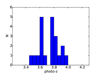
Figure 1.— Distribution of the photometric redshift values obtained running the BPZ code (Benítez, 2000). The narrow distribution matches the redshift window associated with $B_{\rm 435}$-dropout galaxies ($3.4\lesssim z\lesssim 4.4$).

The final samples contain 74 and 428 dropout galaxies for the GOODS v2.0 and HUDF dataset, respectively. It should be noted that the area covered by the GOODS images of the HUDF sky area is almost twice the size of the HUDF sky area, thus several $B_{\rm 435}$-dropouts lie in regions of the image where there is not coverage in the HUDF images. In detail, out of the 74 $B_{\rm 435}$-dropouts detected in GOODS, 48 lie outside the actual HUDF footprint. After obtaining the catalogs of $B_{\rm 435}$-dropouts matching in both datasets, we visually inspected all the sources and rejected any spurious detections. A total of five sources were discarded.

5. Results

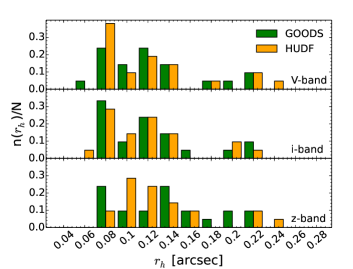
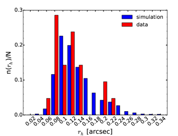
Figure 2.— Left panels: for each detection band the bar plots compare the normalized distribution of values for the half-light radius $r_{h}$ obtained running SExtractor on GOODS-depth (in green) and HUDF-depth (in orange) images. Right panel: bar plots comparing the normalized distribution of half-light radii values from $i_{\rm 775}$-band data (in red) and the simulations (in blue). In detail, we plotted an example of the distribution of half-light radius values recovered by running SExtractor on mock images. All plots are characterized by a bin size of 0.02 arcsec and n($r_{h}$) and N indicate the number of galaxies per bin and the total number of objects analyzed (i.e. 21 in our sample and 1000 in each simulation run), respectively.

Comparing the HUDF data with GOODS v2.0, we obtained a sample of 21 matching objects within the HUDF footprint that were selected as $B_{\rm 435}$-dropout candidates independently in the two datasets. The half-light radii $r_{h}$, derived running SExtractor, are plotted in the left panels of Figure 2. The radii derived from GOODS-depth images and those coming from the HUDF-depth ones are in good agreement.

For all the $B_{\rm 435}$-dropouts in our sample, we plotted the total magnitudes and errors, given by SExtractor MAG_AUTO and MAGERR_AUTO parameters, respectively, and derived the best linear least-squares fit $y=A+B\cdot x$ considering the error bars in both coordinates using the IDL fitexy.pro routine (right panels of Figure 3). The best fit parameters are tabulated in Table 3.

As a further check, we investigated the behavior of all the $B_{\rm 435}$-dropouts selected in HUDF, with no regard for their identification in GOODS v2.0. In particular, we selected all the $B_{\rm 435}$-dropouts detected in HUDF with a total magnitude in the $z_{\rm 850}$-band brighter than $z_{\rm 850}$=26.8 mag, the value that defines the completeness of the GOODS dataset (50% complete). 79 $B_{\rm 435}$-dropouts satisfy this criterion and we focused on them for the following analysis. Discarding the cuts in $S/N$ for the GOODS data, there are 75 objects selected as $B_{\rm 435}$-dropouts in HUDF that have a detection in GOODS v2.0, two of them were discarded as each of them is clearly detected as two distinct sources in GOODS. Out of the 73 remaining objects we ran a separate analysis considering four different cuts in $S/N$ in GOODS-depth images only: $S/N>2$, $S/N>3$, $S/N>4$, $S/N>5$. For each selection we derived the best fit, as done for the sample of matching $B_{\rm 435}$-dropouts.

The left panels of Figure 3 summarize our results plotting the total magnitudes in GOODS and HUDF on the basis of the $S/N$ cut for the different bands. As can be seen from Table 3, there is no significant change in the trend of the linear fit, even including objects with lower $S/N$ detection, showing that deeper images do not reveal any low-SB features, hard to detect due to cosmological dimming, in the sample galaxies. When including the objects with very poor or no detection in at least one of the bands used to identify objects, there could be an effect due to SB dimming, but we are not able to disentangle this effect from the one simply due to the detection limit of GOODS.

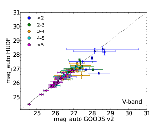
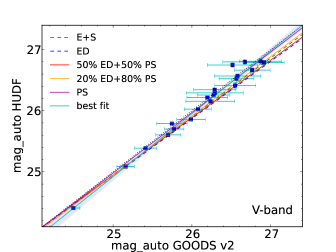
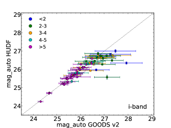
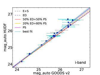
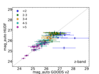
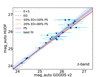
Figure 3.— Total magnitude derived from SExtractor MAG_AUTO parameter in the $V_{\rm 606}$(top panels), $i_{\rm 775}$(central panels), and $z_{\rm 850}$-band (bottom panels) from the GOODS v2.0 dataset compared to the one derived from the HUDF. Left panels refer to all the objects selected in HUDF as $B_{\rm 435}$-dropouts that have a detection in GOODS v2.0. As tabulated in the legend, different colors refer to different cuts in $S/N$ in GOODS if no color selection is applied in GOODS. Right panels show the sample, consisting of 21 $B_{\rm 435}$-dropouts, satisfying all the selection criteria in both HUDF and GOODS v2.0. Since the error bars on the y-axis are small they are often hidden by the symbols. The colored lines indicate the trend if cosmological dimming is acting depending on the way the flux is distributed among the galaxy, while the dotted black line shows the 1:1 trend. The shaded area shows the 95% confidence band around the best fit (solid cyan line). In the legend E, S, ED, and PS indicate ellipticals, spiral galaxies, exponential disk, and point source, respectively.

Table 3Best linear least-square fit

Selection	$V_{\rm 606}$			$i_{\rm 775}$			$z_{\rm 850}$
Criteria	# obj	A	B	# obj	A	B	# obj	A	B
$S/N>5$ + color	21	-0.88	1.03	21	-0.28	1.01	21	-0.45	1.02
$S/N>5$	32	-1.04	1.04	36	-0.59	1.02	20	-1.13	1.04
$S/N>4$	46	-1.13	1.04	45	-0.46	1.02	38	-0.48	1.02
$S/N>3$	58	-0.93	1.03	57	-0.17	1.01	51	-0.67	1.03
$S/N>2$	65	-0.86	1.03	68	0.30	0.99	66	-0.51	1.02
All	73	-0.58	1.02	73	0.56	0.98	73	-0.03	1.00

NOTES: Parameters for the best linear least-square fit in the form $y=A+B\cdot x$. In the fit equation $x$ and $y$ are MAG_AUTO values in GOODS-depth and HUDF-depth, respectively. A and B were derived comparing the total magnitudes in the $V_{\rm 606}$, $i_{\rm 775}$, and $z_{\rm 850}$-band for the sample of matching sources taking into account the error bars associated to the magnitude values. Different rows refer to different selection criteria and, consequently, the number matching of objects varies.

6. Simulations

Our results suggest no effect due to cosmological dimming when comparing deep sky surveys with different depth. To complete our study, we wanted to show that the difference in depth between our two datasets would be enough to detect Tolman dimming effects if galaxies were characterized by a smooth light distribution at the resolution of HST. To this aim, we ran Monte Carlo simulations reproducing the $B_{\rm 435}$-dropout sample in order to derive the expected trend in the magnitude-magnitude plot in the case of cosmological dimming affecting the SB of the sources.

In detail, we created a 4000 x 4000 pixel image in each band into which we inserted 1000 mock galaxies with apparent magnitudes ranging from 24.5 to 28.5 mag, axis ratio $b/a$ and effective radius ${\rm r_{e}}$ distributed according to the findings of Ferguson et al. (2004), and position angle and x,y positions randomly drawn from a flat distribution. We used the noao.artdata.mkobject package in IRAF to make the artificial galaxies. The right panel of Figure 2 shows a comparison between the normalized distribution of the half-light radius values from one of our simulations and our $B_{\rm 435}$-dropout sample. Each value of $r_{h}$ used to create a mock galaxy was drawn from the size distribution presented in Ferguson et al. (2004), that is based on measurements performed by SExtractor on $i_{\rm 775}$-band images. The distribution of the half-light radii, recovered running SExtractor on the i-band image of our dataset, is in good agreement with those recovered from the simulated galaxies.

In the first set of simulations we reproduced the images in each band assuming that all the galaxies have just one component. First we created a mock image containing only disk-like galaxies, i.e. late-type, with a surface brightness exponential profile. We convolved the mock frame with the corresponding PSF model obtained running Tiny Tim (Krist et al., 2011). This tool models the PSF specific to a chosen channel for any of the HST imagers and bands. We obtained three different PSF models, one for each detection band. Finally, we added a random noise frame with the same rms as the one measured on the science image in the corresponding band.

We also created a set of mock images assuming that 25% of the galaxies have a De Vaucouleurs profile (i.e. $r^{1/4}$), and the remaining an exponential one. This is broadly compatible with Ferguson et al. (2004) who found that, among the $B_{\rm 435}$-dropout sample, 78% of the galaxies are classified as late-type. As previously done, we convolved all mock objects with the PSF by Tiny Tim and added random noise.

In both cases, i.e. exponential and mixed profiles, the effect of surface brightness dimming is expected to be large since the objects are extended and the flux is mostly distributed in extended structures.

In the third set of simulations, we used mock galaxies that have a double component. Specifically, we used an exponential disk and a central point source. We used the same PSF image we got from Tiny Tim to convolve the frames as the model for the point source and we convolved only the exponential disks with the typical ACS PSF. As done for the simulations previously described, we added the random noise reproducing the background of the science image in the selected band. In detail, we simulated galaxies with 80% of the flux enclosed in the central point source and 20% in the extended exponential disk or with the flux equally split among the two components.

Finally, we ran the last set of simulations modeling each mock galaxy with the PSF by Tiny Tim, i.e. we created point sources that are not expected to be affected by the curvature $(1+z)^{2}$ component of cosmological dimming. In this case we did not convolve the synthetic frame with the PSF before adding the background noise.

For each set of simulations we performed 50 iterations for each band. Then, we ran SExtractor on each mock image with the same parameters used for the detection in the real data. Finally, we compared the GOODS-depth and HUDF-depth magnitudes for the mock galaxies from the output catalogs. For each realization of the simulations we derived a linear fit describing the expected trend the GOODS-depth magnitude vs HUDF-depth magnitude plot, then we averaged the A and B values over all the 50 realizations in order to derive the best fit parameters listed in Table 4.

To determine whether or not the trends derived from the simulations are in agreement with our data, we computed the normalized residuals for each light distribution profile. In detail, we derived the distance between each data point and the linear fit obtained from a set of simulations and divided it by the corresponding error. For compact sources, for which no significant dimming is expected, we predict the distribution of the residuals to resemble the one obtained with respect to the 1:1 line. Observed objects tend to lie systematically to the left of the model lines (right panels of Figure 3). The residual distribution captures this systematic effect which, instead, can be missed by tests relying only on the squares of the residuals. We performed a Kolmogorov-Smirnov non-parametric statistical test comparing the distribution of the residuals derived from each set of simulations and the one from the data. The values of the maximum vertical deviation between the two cumulative curves, namely the $D$ parameter, and the corresponding probability $p$ are listed in Table 5. If the $p$ value is small, the two groups were sampled from populations with different distributions. We can reject the null hypothesis (i.e. the two distributions are the same) with a 95% confidence for all the realizations characterized by $p<0.05$. As can be seen the expected trend in the cases of flux distributed in extended sources ($r^{1/4}$ and exponential profile) can be easily ruled out in the $V_{\rm 606}$  and $i_{\rm 775}$-band, while the trend for point sources is in agreement with our findings, suggesting that the light from high-$z$ sources mostly comes from compact objects rather than extended ones. It should be noted that diffuse models are ruled out with lower significance in the $z_{\rm 850}$-band and this could hint at a diffuse component starting to be more significant in the redder bands. A compact structure at high-$z$, at least in the bluer bands with a detection, is in agreement with the results obtained by Williams et al. (2014) for $z\sim 3$ LBGs.

As a further result, the simulations involving point sources permitted us to verify the findings of Ashby et al. (2013) who claimed that the total magnitude recovered by SExtractor is, on average, 0.05 mag fainter than the real value. We found all the best fit lines derived for the point source simulations to be slightly shifted in the x direction and that, introducing the 0.05 mag correction stated by Ashby et al. (2013), the fit was closer to the expected trend determined by the 1:1 line.

Table 4Linear least-square fit from Monte Carlo simulations

	Mix (E+S)		exp profile		point source		20% exp profile		50% exp profile
Band	A	B	A	B	A	B	A	B	A	B
$V_{\rm 606}$	0.70	0.97	1.48	0.94	0.20	0.99	0.59	0.97	1.39	0.94
$i_{\rm 775}$	0.74	0.97	1.54	0.94	0.33	0.99	0.64	0.97	1.49	0.94
$z_{\rm 850}$	1.01	0.96	1.67	0.93	0.39	0.98	0.69	0.97	1.75	0.93

NOTES: Best linear least-square fit parameters derived for each of the three detection bands averaging over 50 realizations of Monte Carlo simulations. We considered different scenarios on the basis of the distribution of the total flux: a mix of galaxies (25% with $r^{1/4}$ profile and 75% described by an exponential disk), an exponential disk, a point source modeled using the PSF image created using Tiny Tim, and, finally, multi-component objects with the flux divided into an exponential disk and a point source modeled using Tiny Tim PSF. In particular we considered two cases: either the light equally split among the disk and point source components or 20% of the light in the exponential disk and 80% in the central point source.

Table 5Results from the Kolmogorov-Smirnov statistic

	$V_{\rm 606}$-band		$i_{\rm 775}$-band		$z_{\rm 850}$-band
Profile	$D$	$p$	$D$	$p$	$D$	$p$
Mix (E+S)	0.57	1.08e-03	0.43	0.03	0.42	0.03
Exponential disk	0.67	7.13e-05	0.57	1.08e-03	0.33	0.15
50% Disk + 50% PS	0.62	2.90e-04	0.66	7.10e-05	0.43	0.03
20% Disk + 80% PS	0.52	3.59e-03	0.48	0.01	0.38	0.07
Point source	0.24	0.53	0.29	0.30	0.14	0.97

NOTES: Results from the Kolmogorov-Smirnov test obtained comparing the distribution of the residuals derived from each set of simulations and the one from the data. The values of the $D$ parameter and the corresponding probability $p$ are listed for all the models and bands, as labeled. When $p<0.05$ the distribution of the residuals differ from the expected one with a 95% confidence, so the model can be ruled out as a possible fit for our data.

7. Conclusions

To study the effects of surface brightness dimming on high-redshift galaxies, we compared catalogs of candidate $B_{\rm 435}$-dropouts obtained running SExtractor on deep images taken with ACS as part of the GOODS and HUDF projects. In particular, considering the total magnitude, given by the MAG_AUTO parameter, we found no systematic differences between GOODS and the deeper images from HUDF. In detail, our sample of $B_{\rm 435}$-dropouts suggests that there is no trend in the magnitude of galaxies becoming brighter in the HUDF, as already stated by Beckwith et al. (2006).

If most of the light of faint dropout galaxies was in compact knots, one would expect little or no SB dimming. In contrast, if a substantial fraction of the light is in a diffuse component, such components would be detected in part in the HUDF and missed in GOODS. Our direct comparison shows that galaxies detected in GOODS do not become significantly brighter in deeper images. This finding suggests that most of their light is compact, as claimed by Bouwens et al. (2004) who found that the principal effect of depth in a galaxy survey is to add galaxies at fainter magnitudes, and not to significantly add to the sample galaxies with bigger sizes. Furthermore, our findings are in agreement with those by Williams et al. (2014). Studying the morphology of these galaxies in the rest-frame UV and in the optical, they found a very compact main structure and basically no diffuse component, even in deep stacks.

Comparing the data to simulations reproducing the effect of cosmological dimming for different SB profiles, we found that our trends can not be ascribed to extended structures, such as $r^{1/4}$ profiles or exponential disks. However, diffuse models are ruled out with lower significance in the reddest band, i.e. $z_{\rm 850}$-band, which could hint at a diffuse component starting to be more significant.

The study of cosmological SB dimming is also important since it could affect our prediction of what JWST can observe at higher redshifts, where younger galaxies may exhibit a larger fraction of clumpiness. Our direct comparison shows that galaxies detected in GOODS do not become significantly brighter in the HUDF. This suggests that most of their light is compact and hints at the fact that JWST will likely not find extensive diffuse star forming components. This is also promising as it suggests that JWST will not be confusion limited at least in the shortest bands.

Whether or not galaxies have a red diffuse component remains an open question and will require further investigations.

References

- Ashby et al. (2013) Ashby, M. L. N., Stanford, S. A., Brodwin, M., et al. 2013, ApJS, 209, 22
- Beckwith et al. (2006) Beckwith, S. V. W., Stiavelli, M., Koekemoer, A. M., et al. 2006, AJ, 132, 1729
- Benítez (2000) Benítez, N. 2000, ApJ, 536, 571
- Bertin & Arnouts (1996) Bertin, E., & Arnouts, S. 1996, A&AS, 117, 393
- Bouwens et al. (2004) Bouwens, R. J., Illingworth, G. D., Blakeslee, J. P., Broadhurst, T. J., & Franx, M. 2004, ApJ, 611, L1
- Calvi et al. (2013) Calvi, V., Pizzella, A., Stiavelli, M., et al. 2013, MNRAS, 432, 3474
- Casertano et al. (2000) Casertano, S., de Mello, D., Dickinson, M., et al. 2000, AJ, 120, 2747
- Disney & Lang (2012) Disney, M. J., & Lang, R. H. 2012, MNRAS, 426, 1731
- Ferguson et al. (2004) Ferguson, H. C., Dickinson, M., Giavalisco, M., et al. 2004, ApJ, 600, L107
- Giavalisco (2002) Giavalisco, M. 2002, ARA&A, 40, 579
- Giavalisco et al. (2004) Giavalisco, M., Ferguson, H. C., Koekemoer, A. M., et al. 2004, ApJ, 600, L93
- Huang et al. (2013) Huang, K.-H., Ferguson, H. C., Ravindranath, S., & Su, J. 2013, ApJ, 765, 68
- Krist et al. (2011) Krist, J. E., Hook, R. N., & Stoehr, F. 2011, in Society of Photo-Optical Instrumentation Engineers (SPIE) Conference Series, Vol. 8127, Society of Photo-Optical Instrumentation Engineers (SPIE) Conference Series
- Lanzetta et al. (2002) Lanzetta, K. M., Yahata, N., Pascarelle, S., Chen, H.-W., & Fernández-Soto, A. 2002, ApJ, 570, 492
- Lotz et al. (2006) Lotz, J. M., Madau, P., Giavalisco, M., Primack, J., & Ferguson, H. C. 2006, ApJ, 636, 592
- Oesch et al. (2010) Oesch, P., Bouwens, R. J., Carollo, M., Illingworth, G. D., & HUDF09 Team. 2010, in Bulletin of the American Astronomical Society, Vol. 41, Bulletin of the American Astronomical Society, 532–+
- Oesch et al. (2007) Oesch, P. A., Stiavelli, M., Carollo, C. M., et al. 2007, ApJ, 671, 1212
- Oke & Gunn (1983) Oke, J. B., & Gunn, J. E. 1983, ApJ, 266, 713
- Pascarelle et al. (1998) Pascarelle, S. M., Lanzetta, K. M., & Fernández-Soto, A. 1998, ApJ, 508, L1
- Phillipps et al. (1990) Phillipps, S., Davies, J. I., & Disney, M. J. 1990, MNRAS, 242, 235
- Riess et al. (2007) Riess, A. G., Strolger, L.-G., Casertano, S., et al. 2007, ApJ, 659, 98
- Steidel et al. (1999) Steidel, C. C., Adelberger, K. L., Giavalisco, M., Dickinson, M., & Pettini, M. 1999, ApJ, 519, 1
- Stiavelli (2009) Stiavelli, M. 2009, From First Light to Reionization: The End of the Dark Ages
- Tolman (1930) Tolman, R. C. 1930, Proceedings of the National Academy of Science, 16, 511
- Tolman (1934) —. 1934, Relativity, Thermodynamics, and Cosmology
- Vanzella et al. (2005) Vanzella, E., Cristiani, S., Dickinson, M., et al. 2005, A&A, 434, 53
- Williams et al. (2014) Williams, C. C., Giavalisco, M., Cassata, P., et al. 2014, ApJ, 780, 1