Spicing up continuum solvation models with SaLSA:
the spherically-averaged liquid susceptibility ansatz
Abstract
Continuum solvation models enable electronic structure calculations of systems in liquid environments, but because of the large number of empirical parameters, they are limited to the class of systems in their fit set (typically organic molecules). Here, we derive a solvation model with no empirical parameters for the dielectric response by taking the linear response limit of a classical density functional for molecular liquids. This model directly incorporates the nonlocal dielectric response of the liquid using an angular momentum expansion, and with a single fit parameter for dispersion contributions it predicts solvation energies of neutral molecules with an RMS error of 1.3 kcal/mol in water and 0.8 kcal/mol in chloroform and carbon tetrachloride. We show that this model is more accurate for strongly polar and charged systems than previous solvation models because of the parameter-free electric response, and demonstrate its suitability for ab initio solvation, including self-consistent solvation in quantum Monte Carlo calculations.
Electronic density functional theory Hohenberg and Kohn (1964); Kohn and Sham (1965) enables first-principles prediction of material properties at the atomic scale including structures and reaction mechanisms. Liquids play a vital role in many systems of technological and scientific interest, but the need for thermodynamic phase-space sampling complicates direct first-principles calculations. Further, absence of dispersion interactions and neglect of quantum-mechanical effects in the motion of protons limit the accuracy of ab initio molecular dynamics for solvents such as water Grossman et al. (2004); Morrone and Car (2008).
Continuum solvation models replace the effect of the solvent by the response of an empirically-determined dielectric cavity. Traditional solvation models Fortunelli and Tomasi (1994); Barone et al. (1997); Tomasi et al. (2005); Cramer and Truhlar (1991); Marenich et al. (2007, 2009) employ a large number of atom-dependent parameters, are highly accurate in the class of systems to which they are fit - typically organic molecules in solution, and have been tremendously successful in the evaluation of reaction mechanisms and design of molecular catalysts. Unfortunately, the large number of parameters precludes the extrapolation of these models to systems outside their fit set, such as metallic or ionic surfaces in solution. Recent solvation models that employ an electron-density based parametrization Andreussi et al. (2012); Letchworth-Weaver and Arias (2012) require only two or three parameters and extrapolate more reliably, but still encounter difficulties for charged and highly polar systems Dupont et al. (2013); Gunceler et al. (2013).
The need for empirical parameters in continuum solvation arises primarily because of the drastic simplification of the nonlocal and nonlinear response of the real liquid with that of a continuum dielectric cavity. Recently, we correlated the dielectric cavity sizes for different solvents with the extent of nonlocality of the solvent response to enable a unified electron-density parametrization for multiple solvents Sundararaman et al. , but the electron density threshold that determines the cavity size still required a fit to solvation energies of organic molecules. Joint density functional theory (JDFT) Petrosyan et al. (2007) combines a classical density functional description of the solvent with an electronic density functional description of the solute, naturally captures the nonlocal response of the fluid, and does not involve cavities that are fit to solvation energies.
Here, we derive a nonlocal continuum solvation model from the linear response limit of JDFT. Because there are no fit parameters for the electrostatic response, this theory is therefore suitable for the study of charged and strongly polar systems. This derivation begins with a simple ansatz: the distribution of solvent molecules starts out isotropic and uniform outside a region excluded by the solute; electrostatic interactions between the solute and solvent then perturb this distribution to first order. We first describe a method to estimate that initial distribution from the overlap of solute and solvent electron densities, and then show how to calculate the nonlocal linear response of the fluid using an angular momentum expansion. The addition of nonlocal cavity formation free energy and dispersion functionals derived from classical density functional theory Sundararaman et al. results in an accurate description of solvation free energies of neutral organic molecules as well as highly polar and ionic systems. Finally, we show that the nonlocal dependence of this model on the solute electron density enables self-consistent solvation in quantum Monte-Carlo calculations, which was previously impractical due to statistical noise in the local electron density Schwarz et al. (2012).
I Iso-density-product cavity determination
A common ingredient in continuum solvation models is the formation of a cavity that excludes the solvent from a region of space occupied by the solute. Atom-based parametrizations typically exclude the centers of solvent molecules from a union of spheres centered on each solute atom with radius equal to the sum of the atomic and solvent van-der-Waals (vdW) radii, and then construct a dielectric cavity that is smaller by an empirical solvent-dependent radius Tomasi et al. (2005). In contrast, the density-based approaches adopt a smoothly-varying dielectric constant which is a function of the local solute electron density that switches from the vacuum to bulk solvent value at a solvent-dependent critical electron density Andreussi et al. (2012); Letchworth-Weaver and Arias (2012).
Here, since we explicitly account for the nonlocal response, we require only the distribution of the solvent molecule centers. Because the distance of these centers from the solute atoms corresponds to the distance of nearest approach of two non-bonded systems, vdW radii, which are defined in terms of non-bonded approach distances Mantina et al. (2009), provide a reasonable guess. However, directly using the vdW radii does not account for changes in the electronic configuration between the isolated atom and molecules or solids. A description based on the electronic density would instead naturally capture this dependence.
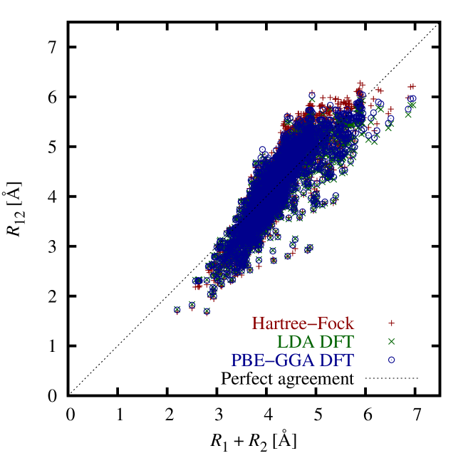
The interaction of non-bonded systems is dominated by Pauli repulsion at short distances, which depends on the overlap of the electron densities of the two systems. Indeed, Figure 1 shows that the atom separation, , at which the electron density overlap crosses a threshold value of correlates well with the sum of vdW radii Haynes (2012) of the two atoms. Here, and are spherical electron densities of the two atoms (calculated using OPIUM OPIUM ), centered apart, and we obtain by minimizing . This result is insensitive to the choice of exchange-correlation approximation used to calculate the densities: at the optimized , the RMS relative error in compared to is for the local-density approximation Perdew and Zunger (1981), for the PBE generalized-gradient approximation Perdew et al. (1996) and for Hartree-Fock theory.
The above analysis provides a universal threshold on the density product that can estimate the approach distance of non-bonded systems. We utilize this capability to determine the distribution of solvent molecule centers around a solute with electron density . Our ansatz requires a spatially-varying but isotropic initial distribution of molecules. Therefore we compute overlaps with the spherically-averaged electron density , where is the electron density of a single solvent molecule and is a unit vector. Following Gunceler et al. (2013), we describe the spatial variation of the solvent distribution by the smooth ‘cavity shape’ functional
| (1) |
which smoothly transitions from vacuum () to bulk fluid () as the overlap of the solute and solvent electron densities (readily calculated as a convolution) crosses the universal overlap threshold .
II Nonlocal electric response
We begin with the in-principle exact joint density-functional description Petrosyan et al. (2007) of the free energy of a solvated electronic system
| (2) |
where is the Hohenberg-Kohn functional Hohenberg and Kohn (1964) of the solute electronic density , is a free energy functional for the solvent in terms of nuclear site densities , and captures the free energy of interaction between the solute and solvent. (See Petrosyan et al. (2007) for details about the theoretical framework.)
We adopt the Kohn-Sham prescription Kohn and Sham (1965) with an approximate exchange-correlation functional for and the polarizable ‘scalar-EOS’ free energy functional approximation Sundararaman et al. (2014) for . We separate in (2) as the mean-field electrostatic interaction and a remainder that is dominated by electronic repulsion and dispersion interactions. We then assume that the remainder is responsible for determining the initial isotropic distribution of solvent molecules, where is the bulk number density of solvent molecules and is given by (1). Substituting the free energy functional from Sundararaman et al. (2014), we can then write (2) as
| (3) |
Above, analogously to the Kohn-Sham approach, the liquid free energy functional employs the state of the corresponding non-interacting system specified by two sets of independent variables. The first, , is the orientation probability density of finding a solvent molecule centered at with orientation SO(3). The solvent site densities are dependent variables that are calculated from . The second variable is the polarization density, for each solvent site.
The second term in (3), , collects all the free energy contributions due to the initial isotropic distribution, so that all the subsequent terms are zero when and . The third term is the non-interacting rotational entropy at temperature , the fourth term is a weighted-density correlation functional for dipole rotations, and the fifth term is the potential energy for molecular polarization with site susceptibilities . and parametrize correlations in the rotations and polarization respectively, and are constrained by the bulk static and optical dielectric constants. The final term is the mean-field interaction between the solute charge density and the induced charge density in the liquid (where is the charge in the initial isotropic distribution), and the self energy of that induced charge. Here,
| (4) |
where and respectively specify decomposition of the solvent molecule’s charge density and nonlocal susceptibility into spherical contributions at the solvent sites. Bulk experimental properties of the liquid and ab initio calculations of a single solvent molecule constrain all involved parameters. See Sundararaman et al. (2014) for details; the terms above are identical, except for the inclusion of solute-solvent interactions in the final electrostatic term and for the separation of the initial isotropic contributions into .
Next, we treat the orientation-dependent pieces perturbatively by expanding , where are the Wigner -matrices (irreducible representations of SO(3)) Wigner (1959). We then expand the free energy (3) to quadratic order in the independent variables (rotation) and (polarization), formally solve the corresponding linear Euler-Lagrange equations and substitute those solutions back into the quadratic form. After some tedious but straightforward algebra involving orthogonality of -matrices, addition of spherical harmonics and their transformation under the -matrices, as well as Fourier transforms to simplify convolutions, we can show that the resulting free energy to second order is exactly
| (5) |
Here, is the Coulomb operator and is the nonlocal ‘spherically-averaged liquid susceptibility’ (SaLSA), expressed conveniently in reciprocal space as
| (6) |
where is the Fourier transform of for any . The first term of (6) captures the polarization response, where is the site density at the initial configuration of a solvent site at a distance from the solvent molecule center. The second term of (6) captures the rotational response of solvent molecules with charge distribution , decomposed in Fourier space as . The prefactor , the dipole rotation correlation factor Sundararaman et al. (2014) for , and it equals unity for all other .
For practical calculations, we rewrite the last term of (5) as , where is the electrostatic potential in vacuum and is the total (mean-field) electrostatic potential which solves the modified Poisson-like equation . The rotational and polarization terms in have the structure which resembles the Poisson equation for an inhomogeneous dielectric, except for the convolutions that introduce the nonlocality. For neutral solvent molecules, the term captures the interaction of the solute with a spherical charge distribution of zero net charge, and is zero except for small contributions from non-zero but negligible overlap of the solute and solvent charges. However, note that the SaLSA response easily generalizes to mixtures, and for ionic species in the solution, the terms convert the Poisson-like equation to a Helmholtz-like equation that naturally captures the Debye-screening effects of electrolytes as in Kendra-PCM. The terms resemble (nonlocal versions of) higher-order differential operators and capture interactions with higher-order multipoles of the solvent molecule, which decrease in magnitude with increasing . We find that including terms up to is sufficient to converge the solvation energies to 0.1 kcal/mol.
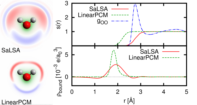
The nonlocality of the SaLSA response allows the fluid bound charge to appear at a distance from the edge of the cavity. For example, for a water molecule in liquid water, the SaLSA cavity transitions at about the first peak of the radial distribution function of water (Figure 2), whereas the bound charge is dominant at smaller distances. In contrast, local solvation models require a smaller unphysical cavity to produce bound charge at the appropriate distance to capture the experimental solvation energy. This key difference from the local models allows a non-empirical description of the electric response in SaLSA.
At this stage, the solvated free energy (5) is fully specified except for the free energy of the initial configuration , dominated by electronic repulsion, dispersion and the free energy of forming a cavity in the liquid. We set , where is a non-local weighted density approximation to the cavity formation free energy and empirically accounts for dispersion and the remaining contributions, exactly as in Sundararaman et al. . (See Sundararaman et al. for a full specification.) Briefly, is completely constrained by bulk properties of the solvent including density, surface tension and vapor pressure, and reproduces the classical density functional and molecular dynamics predictions for the cavity formation free energy from Sundararaman et al. (2014) with no fit parameters. employs a semi-empirical pair potential dispersion correction Grimme (2006) which includes a scale parameter , which we fit to solvation energies below. Note, however, that unlike previous continuum solvation models, the dominant electrostatic response includes no parameters that are fit to solvation energies.
III Solvation energies
We implement the SaLSA solvation model in the open source density-functional software JDFTx Sundararaman et al. (2012), and perform calculations using norm-conserving pseudopotentials OPIUM at 30 plane-wave cutoff and the revTPSS meta-generalized-gradient exchange-correlation functional Perdew et al. (2009). For three solvents, water, chloroform and carbon tetrachloride, we fit the sole parameter to minimize the RMS error in the solvation energies of a small but representative set of neutral organic molecules with a variety of functional groups and chain lengths (same set for each solvent as in Sundararaman et al. ). Table 1 summarizes the optimum values of and the corresponding RMS error in solvation energies. The RMS errors of SaLSA are only slightly higher than those of the local solvation model from Sundararaman et al. that includes additional fit parameters for the electric response.
| Solvent | RMS error [kcal/mol (m)] | ||
|---|---|---|---|
| SaLSA | Local model Sundararaman et al. | ||
| HO | 0.50 | 1.3 (2.0) | 1.1 (1.8) |
| CHCl | 0.88 | 0.7 (1.1) | 0.6 (1.0) |
| CCl | 1.06 | 0.8 (1.3) | 0.5 (0.8) |
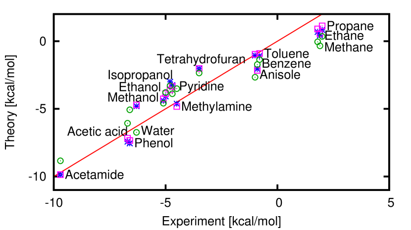
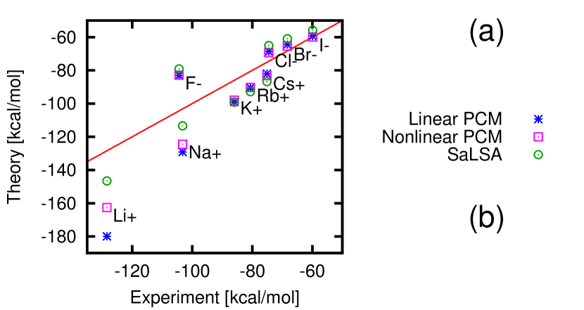
Figure 3 compares the aqueous solvation energy predictions of SaLSA with those of the linear and nonlinear local-response models from Gunceler et al. (2013). All three models perform comparably for the neutral molecule set (Figure 3(a)) used for the parameter fit, but SaLSA is substantially more accurate for inorganic ions (Figure 3(b)). In particular, the local models severely over-predict the solvation energies of small cations, and the nonlocal SaLSA model reduces the error by a factor of three for Li+ and Na+. However, SaLSA does not correct the systematic over-solvation of cations compared to anions, a known deficiency of electron-density based solvation models Dupont et al. (2013).
Finally, we turn to solvation in diffusion quantum Monte-Carlo (DMC) calculations. Conventional density-based solvation models Andreussi et al. (2012); Dupont et al. (2013); Letchworth-Weaver and Arias (2012); Gunceler et al. (2013) are sensitive to the electron density in the low density regions of space ( ). This sensitivity imposes extremely stringent restrictions on the statistical noise in the DMC electron density, rendering self-consistent solvated DMC calculations impractical. A scheme correct to first order that combines a solvated density-functional calculation with a DMC calculation in an external potential provides reasonable accuracy without calculating DMC electron densities Schwarz et al. (2012). However, full self-consistency would be particularly important for systems where density-functional approximations fail drastically.
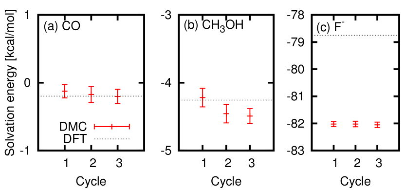
The nonlocality of the SaLSA model, particularly the dependence of the cavity shape (1) on a convolution of the density rather than the local density, significantly reduces its sensitivity to noise in the electron density, and enables self-consistent DMC solvation in a straightforward manner. We start with an initial guess for the density (from solvated DFT), compute the potential on the electrons from the SaLSA fluid model, and perform a DMC calculation (using the CASINO program Needs et al. (2010)) in that external potential while collecting electron density (using the mixed estimator in Needs et al. (2010)). We then mix the DMC electron density with the previous guess, update the fluid potential and repeat till the density becomes self-consistent. The estimation of the solvated energy at each cycle proceeds exactly as in Schwarz et al. (2012) with slight differences in the details of the DMC calculation: we use Trail-Needs pseudopotentials Trail and Needs (2005a, b) with a DFT plane-wave cutoff of 70 , and a DMC time step of 0.004 .
Figure 4 shows that the solvated DMC energy converges to within 0.1 kcal/mol in just three self-consistency cycles. The solvation energies of methanol and carbon monoxide are essentially unchanged from the density-functional results, whereas the solvation energy of the fluoride anion, which suffers from strong self-interaction errors in DFT, is corrected by 3 kcal/mol. This change, although in the right direction, is small compared to the 20 kcal/mol error in the predicted SaLSA solvation energy using DFT (Figure 3(b)). The error in the solvation of anions is therefore not predominantly caused by the inaccuracy of electronic density-functional approximations for anions.
IV Conclusions
The linear-response limit of joint density-functional theory, combined with an electron-density overlap based estimate of the initial solvent molecule distribution, provides a nonlocal continuum solvation model with no empirical parameters for the electric response. Consequently, this ‘SaLSA’ model extrapolates more reliably from neutral organic molecules to ions and is an excellent candidate for describing highly polar and charged surfaces in solution. Further, the nonlocality of this model enables self-consistent solvation in diffusion Monte Carlo calculations. This opens up the possibility of studying systems in solution for which standard density-functional approximations fail, such as the adsorption of carbon monoxide on transition metal surfaces. Additionally, SaLSA should facilitate the development of more accurate and perhaps more empirical models that, for example, account for the charge asymmetry in the solvation of cations and anions.
This work was supported as a part of the Energy Materials Center at Cornell (EMC2), an Energy Frontier Research Center funded by the U.S. Department of Energy, Office of Science, Office of Basic Energy Sciences under Award Number DE-SC0001086.
References
- Hohenberg and Kohn (1964) P. Hohenberg and W. Kohn, Phys. Rev. 136, B864 (1964).
- Kohn and Sham (1965) W. Kohn and L. Sham, Phys. Rev. 140, A1133 (1965).
- Grossman et al. (2004) J. C. Grossman, E. Schwegler, E. W. Draeger, F. Gygi, and G. Galli, J. Chem. Phys. 120, 300 (2004).
- Morrone and Car (2008) J. A. Morrone and R. Car, Phys. Rev. Lett. 101, 017801 (2008).
- Fortunelli and Tomasi (1994) A. Fortunelli and J. Tomasi, Chem. Phys. Lett. 231, 34 (1994).
- Barone et al. (1997) V. Barone, M. Cossi, and J. Tomasi, J. Chem. Phys. 107, 3210 (1997).
- Tomasi et al. (2005) J. Tomasi, B. Mennucci, and R. Cammi, Chem. Rev. 105, 2999 (2005).
- Cramer and Truhlar (1991) C. J. Cramer and D. G. Truhlar, J.Am. Chem. Soc. 113, 8305 (1991).
- Marenich et al. (2007) A. V. Marenich, R. M. Olson, C. P. Kelly, C. J. Cramer, and D. G. Truhlar, J. Chem. Theory Comput. , 2011 (2007).
- Marenich et al. (2009) A. V. Marenich, C. J. Cramer, and D. G. Truhlar, J. Phys. Chem. B 113, 6378 (2009).
- Andreussi et al. (2012) O. Andreussi, I. Dabo, and N. Marzari, J. Chem. Phys 136, 064102 (2012).
- Letchworth-Weaver and Arias (2012) K. Letchworth-Weaver and T. A. Arias, Phys. Rev. B 86, 075140 (2012).
- Dupont et al. (2013) C. Dupont, O. Andreussi, and N. Marzari, J. Chem. Phys 139, 214110 (2013).
- Gunceler et al. (2013) D. Gunceler, K. Letchworth-Weaver, R. Sundararaman, K. Schwarz, and T. Arias, Modelling Simul. Mater. Sci. Eng. 21, 074005 (2013).
- (15) R. Sundararaman, D. Gunceler, and T. A. Arias, “Weighted-density functionals for cavity formation and dispersion energies in continuum solvation models,” Preprint arXiv:1407.4011.
- Petrosyan et al. (2007) S. A. Petrosyan, J.-F. Briere, D. Roundy, and T. A. Arias, Phys. Rev. B 75, 205105 (2007).
- Schwarz et al. (2012) K. A. Schwarz, R. Sundararaman, K. Letchworth-Weaver, T. A. Arias, and R. G. Hennig, Phys. Rev. B 85, 201102(R) (2012).
- Haynes (2012) W. M. Haynes, ed., CRC Handbook of Physics and Chemistry 93 ed (Taylor and Francis, 2012).
- Mantina et al. (2009) M. Mantina, A. C. Chamberlin, R. Valero, C. J. Cramer, and D. G. Truhlar, J. Phys. Chem. A 113, 5806 (2009).
- (20) OPIUM, Pseudopotential generation project, http://opium.sf.net.
- Perdew and Zunger (1981) Perdew and Zunger, Phys. Rev. B 23, 5048 (1981).
- Perdew et al. (1996) J. P. Perdew, K. Burke, and M. Ernzerhof, Phys. Rev. Lett. 77, 3865 (1996).
- Sundararaman et al. (2014) R. Sundararaman, K. Letchworth-Weaver, and T. A. Arias, J . Chem. Phys. 140, 144504 (2014).
- Wigner (1959) E. P. Wigner, Group theory and its application to the quantum mechanics of atomic spectra (Academic Press, New York, 1959).
- Soper (2000) A. K. Soper, Chem. Phys. 258, 121 (2000).
- Grimme (2006) S. Grimme, J. Comput. Chem 27, 1787 (2006).
- Sundararaman et al. (2012) R. Sundararaman, K. L.-W. D. Gunceler, and T. A. Arias, “JDFTx,” http://jdftx.sourceforge.net (2012).
- Perdew et al. (2009) J. P. Perdew, A. Ruzsinszky, G. I. Csonka, L. A. Constantin, and J. Sun, Phys. Rev. Lett. 103, 026403 (2009).
- Tannor et al. (1994) D. J. Tannor, B. Marten, R. Murphy, R. A. Friesner, D. Sitkoff, A. Nicholls, M. Ringnalda, W. A. Goddard, and B. Honig, J. Am. Chem. Soc. 116, 11875 (1994).
- Marten et al. (1996) B. Marten, K. Kim, C. Cortis, R. A. Friesner, R. B. Murphy, M. N. Ringnalda, D. Sitkoff, and B. Honig, J. Phys. Chem. 100, 11775 (1996).
- Kelly et al. (2006) C. P. Kelly, C. J. Cramer, and D. G. Truhlar, J. Phys. Chem. B 110, 16066 (2006).
- Needs et al. (2010) R. J. Needs, M. D. Towler, N. D. Drummond, and P. L. Ríos, J. Phys.: Condens. Matter 22, 023201 (2010).
- Trail and Needs (2005a) J. Trail and R. Needs, J. Chem. Phys. 122, 174109 (2005a).
- Trail and Needs (2005b) J. Trail and R. Needs, J. Chem. Phys. 122, 014112 (2005b).