A Meta-analysis of the 8 TeV ATLAS and CMS SUSY Searches

Abstract

Between the ATLAS and CMS collaborations at the LHC, hundreds of individual event selections have been measured in the data to look for evidence of supersymmetry at a center of mass energy of 8 TeV. While there is currently no significant evidence for any particular model of supersymmetry, the large number of searches should have produced some large statistical fluctuations. By analyzing the distribution of p-values from the various searches, we determine that the number of excesses is consistent with the Standard Model only hypothesis. However, we do find a shortage of signal regions with far fewer observed events than expected in both the ATLAS and CMS datasets (at $1.65\sigma$ and $2.77\sigma$, respectively). While not as compelling as a surplus of excesses, the lack of deficits could be a hint of new physics already in the 8 TeV datasets.

1 Introduction

The 2012 discovery of the Higgs boson by the ATLAS Aad:2012tfa and CMS Chatrchyan:2012ufa experiments at the Large Hadron Collider (LHC) brought widespread attention to the field of high energy physics. The discovery also reaffirmed the existence of the hierarchy problem due to the small value of the Higgs boson mass. One popular solution to the hierarchy problem is Supersymmetry (SUSY), in which every Standard Model (SM) particle has a supersymmetric counterpart. Since no SUSY particles have been observed, SUSY must be broken: the SUSY partner masses are much larger than their SM analogues. However, the LHC provides a large center of mass energy which could be high enough to produce some of these SUSY particles. Both ATLAS and CMS have conducted extensive searches for SUSY in a multitude of final states, with various numbers of jets, leptons, and photons. The kinematic reach of the detectors have been exploited in order to be sensitive to high mass particles, which may be produced with a low cross section.

Every search for SUSY consists of three pieces: 1) an event selection to maximize sensitivity to a particular model of interest, 2) an estimation of the number of SM events which will pass the selection for a given amount of data, and 3) a comparison of the measured number of events in the region with the predicted number. As the data are stochastic, the last step requires a statistical analysis which incorporates the systematic uncertainties in the predicted event yields. For a particular statistical model of the SM prediction, if the probability $p$ that the measurement could have been generated from the prediction is small, then one has evidence for SUSY. One usually converts the value $p$ into a Gaussian equivalent number of standard deviations and then the generally agreed upon threshold for ‘evidence’ is $3\sigma$ and for ‘discovery’ is $5\sigma$. However, both ATLAS and CMS have performed many searches. In particular, each analysis usually involves many selections and so there are hundreds of searches between the two collaborations. Statistical fluctuations alone should then lead to several high $n\sigma$ measurements. By studying the distribution of p-values, we analyze the compatibility of the 8 TeV ATLAS and CMS SUSY searches with the SM-only hypothesis. The procedure is similar to the analysis of the 7 TeV SUSY searches NachmanRudelius , with a few additions that are discussed in the analysis and results sections.

2 Constructing the Dataset

Even though the 8 TeV dataset was collected in 2012, both ATLAS and CMS are continuing to analyze the data. Most likely, searches will continue to become public until the 14 TeV run efforts are fully operational in the beginning of 2015. Therefore, we arbitrarily cutoff the searches considered for this analysis at the SUSY 2014 conference (July 20, 2014). This includes 17 ATLAS papers Aad:2014nra ; Aad:2014mra ; Aad:2014lra ; Aad:2014kra ; Aad:2014yka ; Aad:2014bva ; Aad:2014wea ; Aad:2014iza ; Aad:2014pda ; Aad:2014vma ; Aad:2014mha ; Aad:2014qaa ; Aad:2014nua ; Aad:2013gva ; Aad:2013yna ; Aad:2013ija ; Aad:2013wta and 12 CMS papers Khachatryan:2014qwa ; Khachatryan:2014doa ; Chatrchyan:2014aea ; Chatrchyan:2014lfa ; Chatrchyan:2013mya ; Chatrchyan:2013fea ; Chatrchyan:2013iqa ; Chatrchyan:2013xna ; Chatrchyan:2013xsw ; Chatrchyan:2013wxa ; Chatrchyan:2013lya ; Chatrchyan:2012paa . The difficulty in assembling the dataset for the present analysis is to understand the correlations between measurements. The general strategy is to categorize the various searches by their selections on jets, leptons, and photons. Two analyses which have non-overlapping requirements in the number and properties of these objects are treated as uncorrelated. For the data, this is an excellent assumption and only breaks down in the rare case that the data in one signal region is used for the background estimate of another signal region. If two signal regions are such that one is a subset of the other, then a decorrelation procedure is attempted in order to produce two orthogonal regions. If the yields are $x\pm\sigma_{x}$ and $y\pm\sigma_{y}$ with $x<y$, then the decorrelated regions have yields $x\pm\sigma_{x}$ and $(y-x)\pm\sqrt{\sigma_{y}^{2}-\sigma_{x}^{2}}$. In all other cases, it is not possible with the information given to determine the correlations and the signal regions in question are simply not used. In general, if there are two analyses with an unknown correlation, the one with more signal regions is preferred unless the one with fewer regions already has orthogonal selections. Tables 1 and 2 give some summary information about the dataset construction given the general guidelines from above.

arXiv reference	Category	Note
1303.2985	Multijets	Regions orthogonal; drop those with $H_{T}>800$ GeV due to overlap with 1402.4770
1402.4770	Multijets	Regions orthogonal; drop those with $H_{T}\in[500,800]$ GeV due to overlap with 1303.2985
1305.2390	Multijets	Unknown correlation with 1303.2985 and 1402.4770: remove
1311.4937	One Lepton	Regions orthogonal; use the LS method for uncertainties when given a choice
1308.1586	One Lepton	Unknown correlation with 1311.4937. Prefer 1311.4937 as its regions are orthogonal
1212.6194	Same sign leptons	SR6 $\subseteq$ SR3 $\subseteq$ SR4 $\subseteq$ SR1 $\subseteq$ SR0. Drop other regions.
1311.6736	Same sign leptons	Drop regions with $\geq 2$ b-jets due to overlap with 1212.6194. Arbitrarily pick the low $p_{T}$ region
1306.6643	Multileptons	Unknown overlap with 1404.5801. Use 1404.5801 as it has more regions.
1404.5801	Multileptons	Regions orthogonal.
1405.3886	Multileptons	Use the two lepton OS regions only.
1405.7570	Multileptons	Use the two lepton OS regions only. Use signal sensitive regions (as described in the text)
1312.3310	Diphoton	Regions orthogonal.

Table 1: An overview of the signal regions used in the meta-analysis from 8 TeV CMS searches.

arXiv reference	Category	Note
1308.1841	Multijets	8j80$x$b $\subseteq$ 8j50$x$b, $x\in\{0,1,2\}$. Unknown correlations between $M_{J}^{\Sigma}$ regions and others, drop
1308.2631	Multijets	SRA $m_{CT}(350)$ $\subseteq$ SRA $m_{CT}(300)$ $\subseteq$ $\cdots$ $\subseteq$ SRA $m_{CT}(150)$
1407.0608	Multijets	M3 $\subseteq$ M2 $\subseteq$ M1; C2 $\subseteq$ C1
1405.7875	Multijets	2jt $\subseteq$ 2jm $\subseteq$ 2jl. 2jW $\cap$ 3j unknown, drop 2jW. 6jt $\subseteq$ 6jm $\subseteq$ 5j and 6jl (5j $\cap$ 6jl $=\{\}$ once 6jm is removed). Drop all other regions due to unknown correlations.
1406.1122	Multijets	SRA2 $\subseteq$ SRA1; SRA4 $\subseteq$ SRA3. Drop SRB. SRC3 $\subseteq$ SRC2 $\subseteq$ SRC1
1407.0600	Multijets	SR-0l-7j-C $\subseteq$ B $\subseteq$ A; Drop 4j regions due to 4j $\cap$ 7j = ?
1407.0583	One Lepton	Unknown correlations between shape fit regions, consider only tN_diag (signal sensitive regions). tN_boost $\subseteq$ tN_med $\subseteq$ tightest tN_diag region. bCb_high $\subseteq$ bCb_med1. Unknown relation between bCa_low and bCa_med, drop low. Unknown correlation between bCd, tNbC_mix and other regions, drop
1407.0603	At Least One $\tau$	1$\tau$Tight $\subseteq$ 1$\tau$Loose, 2$\tau$ GMSB $\subseteq$ 2$\tau$ nGM $\subseteq$ 2$\tau$ Incl. Unknown overlap between 2$\tau$ bRPV and 2$\tau$ GM, drop bRPV. $\tau$+l bGM $\subseteq$ $\tau$+l mSUGRA. Unknown overlap between $\tau$+l GMSB and bRPV, drop bRPV
1407.0350	At least two $\tau$s	C1C1 $\cap$ C1N2 = ?, drop C1C1 DS-lowMass $\cap$ DS-highMass = ?, drop lowMass
1403.4853	Two OS Leptons	unknown correlation of L90,120 with 1403.5294, drop unknown correlation between L110-100, drop L100 H160 orthogonal, drop MVA region
1403.5294	Two OS Leptons	Jet veto regions orthogonal to other searches, drop Zjets $m_{T2}^{150}(x)\subseteq m_{T2}^{120}(x)\subseteq WWc(x)\subseteq m_{T2}^{90}(x)$, $x\in\{SF,DF\}$ Overlap of $WWb(x)$ with $m_{T2}^{90}(x)$ unknown, drop
1404.2500	Same Sign Leptons	Regions orthogonal. Drop SR3Llow/high due to unknown overlap with 1402.7029
1403.5222	Multileptons	SR$x$b $\subseteq$ SR$x$a, $x\in\{2,3\}$
1402.7029	Three Leptons	Regions orthogonal except SR2$\tau$a $\cap$ SR2$\tau$b = ?, drop b
1405.5086	$\geq 4$ Leptons	SR$x$noZb $\subseteq$ SR$x$noZa, $x\in\{0,1,2\}$
1310.3675	Disappearing Tracks	Region inclusion by increasing $p_{T}$ cut
1310.6584	Out-of-time	For the muon veto, inclusion by jet $p_{T}$

Table 2: An overview of the signal regions used in the meta-analysis from 8 TeV ATLAS searches. Note that OS = opposite sign. Inclusions for 1407.0583 are an approximation.

3 Analysis

Once the ATLAS and CMS datasets were constructed, the expected and observed distributions of p-values were computed for both a Gaussian and a lognormal distribution of the expected number of counts (the number of counts itself is assumed to be Poisson). A p-value was assigned to each data point according to

$$\mbox{p-value}=\int_{0}^{\infty}{\phi(\lambda|\mu,\sigma)P_{\geq n}(\lambda)d\lambda}.$$ (1)

Here, $P_{\geq n}$ is the probability of observing $n$ or more counts given a Poisson distribution with parameter $\lambda$,

$$P_{\geq n}(\lambda)=\sum_{k=n}^{\infty}\frac{e^{-\lambda}\lambda^{k}}{k!}=1-\sum_{k=0}^{n-1}\frac{e^{-\lambda}\lambda^{k}}{k!}.$$ (2)

We performed a similar analysis of deficits rather than excesses in the SUSY search regions by replacing $P_{\geq n}$ in (1) with $P_{\leq n}$: the probability of observing $n$ or less counts given a Poisson distribution with parameter $\lambda$. The function $\phi(\lambda|\mu,\sigma)$ is the probability distribution function of the specified random variable with mean $\mu$ and standard deviation $\sigma$. These parameters are the expected value for the number of counts ($\mu$) and the uncertainty on that value ($\sigma$). For the Gaussian distribution,

$$\phi(\lambda|\mu,\sigma)=\frac{1}{N\sigma\sqrt{2\pi}}e^{-(\lambda-\mu)^{2}/2\sigma^{2}},$$ (3)

where $N$ is a normalization constant correcting for the fact that $\lambda$ cannot be negative, and so the negative part of the distribution must be cut off. For the lognormal distribution, whose support is $\mathbb{R}_{+}$, no such normalization constant is required,

$$\phi(\lambda|\mu,\sigma)=\frac{1}{\lambda\tilde{\sigma}\sqrt{2\pi}}e^{-(\ln{\lambda}-\tilde{\mu})^{2}/2\tilde{\sigma}^{2}},$$ (4)

with $\tilde{\mu}:=\ln{\mu^{2}/\sqrt{\mu^{2}+\sigma^{2}}}$, $\tilde{\sigma}:=\sqrt{\ln{1+\sigma^{2}/\mu^{2}}}$ defined so that the lognormal distribution is precisely the distribution of $Y=e^{X}$ for a Gaussian random variable $X$ with mean $\tilde{\mu}$ and variance $\tilde{\sigma}^{2}$.

One might expect the distribution of p-values defined in this way to be uniformly distributed on the interval $[0,1]$ under the null hypothesis, in accordance with the usual interpretation of p-values as the probability of observing a more significant result in precisely $p\times 100\%$ of studies. However, this intuitive understanding is only correct when the distribution is continuous Hartung , not in the case of Poisson distribution considered here. As a result, we first computed the expected distribution of p-values under the null hypothesis and then compared this with the observed distribution of p-values. The expected distribution of p-values is determined by summing up the probability that each particular trial would fall into one of ten bins, $(\frac{i}{10},\frac{i+1}{10}],i=0,...,9$,

$$\mbox{Pr}\left(\frac{i}{10}<\mbox{p-value}\leq\frac{i+1}{10}\right)=\int_{0}^{\infty}{d\lambda f_{i}(\lambda)\phi(\lambda|\mu,\sigma)},$$ (5)

where

$$f_{i}(\lambda)=\sum_{m=0}^{\infty}\left[\mbox{Pr}(X=m)\times\left\{\begin{array}[]{lc}1&\mbox{ if }\mbox{Pr}(X\geq m)\in(\frac{i}{10},\frac{i+1}{10}]\\ 0&\mbox{ otherwise }\end{array}\right\}\right].$$ (6)

Here, $X\sim$ Poisson$(\lambda)$ is the random variable measuring the number of counts, and the $\geq$ in (6) is replaced by a $\leq$ when computing deficits below rather than excesses above the expected signal.

Some of the studied signal regions had $0$ expected events. There is no lognormal distribution with a mean of 0, so these regions had to be discarded in performing the lognormal analysis. Fortunately, this only applied to seven of the CMS signal regions and none of the ATLAS ones. However, a fairly sizable fraction had an expected mean that was very close to zero. For these trials, it is reasonable to suspect that neither a Gaussian with a cutoff imposed at $0$ nor a lognormal will provide a good approximation to the true error distribution. As a double check, we repeated our analysis after removing all data points with $\mu-2\sigma<0$ ($\approx 10\%$ for ATLAS, $30\%$ for CMS) . The results of this second analysis did not differ qualitatively from the first, indicating that the results of the original analysis are not significantly affected by the statistical modeling of these data points.

4 Results and Discussion

The results of our analysis are shown in Figures 1-2. The left-hand side of each plot represents ATLAS data, whereas the right-hand side represents CMS data. Figures 1-2 depict excesses above the expected signal for Gaussian and lognormal errors, respectively, whereas Figures 3-4 depict deficits for Gaussian and lognormal errors, respectively. Results of statistical analysis tests for the ATLAS data are shown in Tables 3-4, while CMS results are shown in Tables 5-6.

The observed distributions for the 2014 ATLAS data look very similar to those for the 2014 CMS data. Both exhibit a lack of deficits with $p<0.1$. Statistically, this shortage is only marginally significant for ATLAS with a p-value of $0.10$, indicating a lack of deficits at a level of $1.65\sigma$. For CMS, on the other hand, the p-value is $0.006$, indicating a shortage of deficits at a level of $2.77\sigma$. Furthermore, the CMS dataset displays a lack of deficits with $p<0.3$ at p-value $0.0009$, or equivalently a level of $3.32\sigma$. The data also exhibit a statistically significant lack of p-values in the tails of the excess distribution, though this disappears for the ATLAS data once one considers deficits instead of excesses. The greater statistical significance for the CMS distributions compared with the ATLAS distributions may be reflective of the fact that there were many more data points in the CMS dataset compared with the ATLAS dataset.

It is interesting to note that the distributions observed here are somewhat different from those observed in our analysis of the 7 TeV data NachmanRudelius . That analysis also revealed a deficit of p-values in the tails of the distribution, but there were significantly fewer p-values $<0.1$, indicating a possible overestimation of the mean background as well as the uncertainty. Here, there is actually a slight (statistically insignificant) surplus of p-value excesses $<0.1$ in the Gaussian case, but a clear lack of p-value deficits $<0.1$ in both the Gaussian and lognormal cases. Assuming this is a result of systematic uncertainties rather than unusually large statistical fluctuations, it would indicate one of three things:

1. The uncertainty distributions differ significantly from Gaussian and lognormal distributions with the reported uncertainties and means.

2. The background has been underestimated as a result of biases inherent in the estimation methods.

3. The background has been underestimated as a result of new physics.

The present analysis cannot distinguish between these three possibilities. At the least, the differences indicate that the true uncertainty distributions are not well described by Gaussian or lognormal distributions with the reported means and uncertainties. We therefore encourage future SUSY data searches to publish their uncertainty distributions to ensure proper interpretation of the results and more powerful analyses of the data.

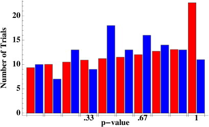
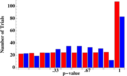
Figure 1: Observed (blue) vs. expected (red) distribution of p-value excesses with a Gaussian error distribution for ATLAS (left) and CMS (right).

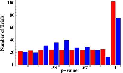
Figure 2: Observed (blue) vs. expected (red) distribution of p-value excesses with a lognormal error distribution for ATLAS (left) and CMS (right).

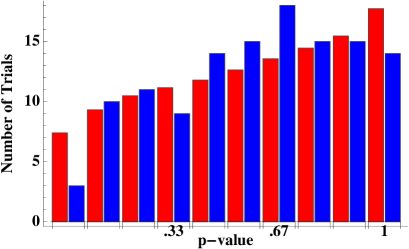
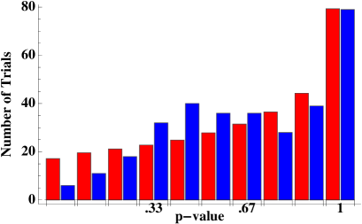
Figure 3: Observed (blue) vs. expected (red) distribution of p-value deficits with a Gaussian error distribution for ATLAS (left) and CMS (right).

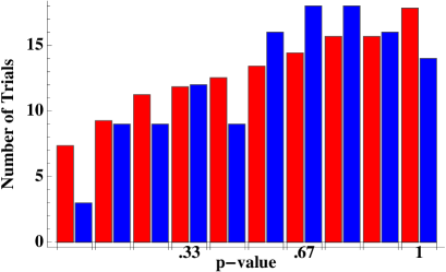
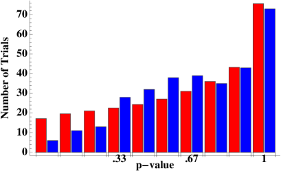
Figure 4: Observed (blue) vs. expected (red) distribution of p-value deficits with a lognormal error distribution for ATLAS (left) and CMS (right).

Quantity	Dist. under $H_{0}$ ($T$)	Test statistic ($t$)		Pr($|T|>t$)
		Gaussian	LN	Gaussian	LN
Trials with $p<0.1$	N(0,1)	0.22	$-0.11$	0.83	0.91
Trials with $p<0.3$	N(0,1)	0.03	0.23	0.73	0.82
Trials with $p<0.2$ or $p>0.8$	N(0,1)	$-2.56$	$-2.55$	0.01	0.01
Expected vs. observed dist.	$\chi^{2}_{9}$	13.65	17.49	0.14	0.04

Table 3: Results for statistical hypothesis tests on ATLAS excesses, under the assumptions of Gaussian and lognormal error distributions. The distribution is significantly different from expected due to the dearth of observed p-values between $0.9$ and $1.0$.

Quantity	Dist. under $H_{0}$ ($T$)	Test statistic ($t$)		Pr($|T|>t$)
		Gaussian	LN	Gaussian	LN
Trials with $p<0.1$	N(0,1)	$-1.66$	$-1.65$	0.10	0.10
Trials with $p<0.3$	N(0,1)	$-0.70$	$-1.48$	0.49	0.14
Trials with $p<0.2$ or $p>0.8$	N(0,1)	$-1.45$	$-1.49$	0.15	0.14
Expected vs. observed dist.	$\chi^{2}_{9}$	6.23	6.59	0.72	0.68

Table 4: Results for statistical hypothesis tests on ATLAS deficits, under the assumptions of Gaussian and lognormal error distributions. The lack of p-values below $0.1$ is marginally significant, while the remainder of the tests are insignificant.

Quantity	Dist. under $H_{0}$ ($T$)	Test statistic ($t$)		Pr($|T|>t$)
		Gaussian	LN	Gaussian	LN
Trials with $p<0.1$	N(0,1)	0.13	$-0.25$	0.90	0.80
Trials with $p<0.3$	N(0,1)	$-0.56$	0.35	0.57	0.73
Trials with $p<0.2$ or $p>0.8$	N(0,1)	$-4.66$	$-4.82$	$\ll 0.001$	$\ll 0.001$
Expected vs. observed dist.	$\chi^{2}_{9}$	28.75	33.33	0.001	$\ll 0.001$

Table 5: Results for statistical hypothesis tests on CMS excesses, under the assumptions of Gaussian and lognormal error distributions.

Quantity	Dist. under $H_{0}$ ($T$)	Test statistic ($t$)		Pr($|T|>t$)
		Gaussian	LN	Gaussian	LN
Trials with $p<0.1$	N(0,1)	$-2.77$	$-2.78$	0.006	0.005
Trials with $p<0.3$	N(0,1)	$-3.32$	$-4.05$	0.0009	$\ll 0.001$
Trials with $p<0.2$ or $p>0.8$	N(0,1)	$-2.81$	$-2.55$	0.005	$0.01$
Expected vs. observed dist.	$\chi^{2}_{9}$	30.09	24.39	$\ll 0.001$	0.003

Table 6: Results for statistical hypothesis tests on CMS deficits, under the assumptions of Gaussian and lognormal error distributions.

- (1) ATLAS Collaboration, Observation of a new particle in the search for the Standard Model Higgs boson with the ATLAS detector at the LHC, Phys.Lett. B716 (2012) 1–29 [1207.7214].
- (2) CMS Collaboration, Observation of a new boson at a mass of 125 GeV with the CMS experiment at the LHC, Phys.Lett. B716 (2012) 30–61 [1207.7235].
- (3) B. Nachman and T. Rudelius, Evidence for conservatism in LHC SUSY searches, Eur.Phys.J.Plus 127 (2012) 157 [1209.3522].
- (4) ATLAS Collaboration, Search for pair-produced third-generation squarks decaying via charm quarks or in compressed supersymmetric scenarios in collisions at TeV with the ATLAS detector, Phys.Rev. D90 (2014) 052008 [1407.0608].
- (5) ATLAS Collaboration, Search for supersymmetry in events with large missing transverse momentum, jets, and at least one tau lepton in 20 fb-1 of =8 TeV proton-proton collision data with the ATLAS detector, 1407.0603.
- (6) ATLAS Collaboration, Search for strong production of supersymmetric particles in final states with missing transverse momentum and at least three b-jets at 8 TeV proton-proton collisions with the ATLAS detector, 1407.0600.
- (7) ATLAS Collaboration, Search for top squark pair production in final states with one isolated lepton, jets, and missing transverse momentum in 8 TeV pp collisions with the ATLAS detector, 1407.0583.
- (8) ATLAS Collaboration, Search for the direct production of charginos, neutralinos and staus in final states with at least two hadronically decaying taus and missing transverse momentum in collisions at = 8 TeV with the ATLAS detector, 1407.0350.
- (9) ATLAS Collaboration, Search for direct pair production of the top squark in all-hadronic final states in proton-proton collisions at TeV with the ATLAS detector, JHEP 1409 (2014) 015 [1406.1122].
- (10) ATLAS Collaboration, Search for squarks and gluinos with the ATLAS detector in final states with jets and missing transverse momentum using TeV proton–proton collision data, 1405.7875.
- (11) ATLAS Collaboration, Search for supersymmetry in events with four or more leptons in = 8 TeV pp collisions with the ATLAS detector, Phys.Rev. D90 (2014) 052001 [1405.5086].
- (12) ATLAS Collaboration, Search for supersymmetry at =8 TeV in final states with jets and two same-sign leptons or three leptons with the ATLAS detector, JHEP 1406 (2014) 035 [1404.2500].
- (13) ATLAS Collaboration, Search for direct production of charginos, neutralinos and sleptons in final states with two leptons and missing transverse momentum in collisions at 8 TeV with the ATLAS detector, JHEP 1405 (2014) 071 [1403.5294].
- (14) ATLAS Collaboration, Search for direct top squark pair production in events with a Z boson, b-jets and missing transverse momentum in sqrt(s)=8 TeV pp collisions with the ATLAS detector, Eur.Phys.J. C74 (2014) 2883 [1403.5222].
- (15) ATLAS Collaboration, Search for direct top-squark pair production in final states with two leptons in pp collisions at 8TeV with the ATLAS detector, JHEP 1406 (2014) 124 [1403.4853].
- (16) ATLAS Collaboration, Search for direct production of charginos and neutralinos in events with three leptons and missing transverse momentum in 8TeV collisions with the ATLAS detector, JHEP 1404 (2014) 169 [1402.7029].
- (17) ATLAS Collaboration, Search for long-lived stopped R-hadrons decaying out-of-time with pp collisions using the ATLAS detector, Phys.Rev. D88 (2013), no. 11 112003 [1310.6584].
- (18) ATLAS Collaboration, Search for charginos nearly mass degenerate with the lightest neutralino based on a disappearing-track signature in pp collisions at =8 TeV with the ATLAS detector, Phys.Rev. D88 (2013), no. 11 112006 [1310.3675].
- (19) ATLAS Collaboration, Search for direct third-generation squark pair production in final states with missing transverse momentum and two -jets in 8 TeV collisions with the ATLAS detector, JHEP 1310 (2013) 189 [1308.2631].
- (20) ATLAS Collaboration, Search for new phenomena in final states with large jet multiplicities and missing transverse momentum at sqrt(s)=8 TeV proton-proton collisions using the ATLAS experiment, JHEP 1310 (2013) 130 [1308.1841].
- (21) CMS Collaboration, Searches for electroweak production of charginos, neutralinos, and sleptons decaying to leptons and W, Z, and Higgs bosons in pp collisions at 8 TeV, 1405.7570.
- (22) CMS Collaboration, Search for top-squark pairs decaying into Higgs or Z bosons in pp collisions at sqrt(s) = 8 TeV, Phys.Lett. B736 (2014) 371 [1405.3886].
- (23) CMS Collaboration, Search for anomalous production of events with three or more leptons in pp collisions at sqrt(s) = 8 TeV, Phys.Rev. D90 (2014) 032006 [1404.5801].
- (24) CMS Collaboration, Search for new physics in the multijet and missing transverse momentum final state in proton-proton collisions at = 8 TeV, JHEP 1406 (2014) 055 [1402.4770].
- (25) CMS Collaboration, Search for top squark and higgsino production using diphoton Higgs boson decays, Phys.Rev.Lett. 112 (2014) 161802 [1312.3310].
- (26) CMS Collaboration, Search for new physics in events with same-sign dileptons and jets in pp collisions at = 8 TeV, JHEP 1401 (2014) 163 [1311.6736].
- (27) CMS Collaboration, Search for supersymmetry in pp collisions at =8 TeV in events with a single lepton, large jet multiplicity, and multiple b jets, Phys.Lett. B733 (2014) 328–353 [1311.4937].
- (28) CMS Collaboration, Search for top-squark pair production in the single-lepton final state in pp collisions at = 8 TeV, Eur.Phys.J. C73 (2013) 2677 [1308.1586].
- (29) CMS Collaboration, Search for top squarks in -parity-violating supersymmetry using three or more leptons and b-tagged jets, Phys.Rev.Lett. 111 (2013), no. 22 221801 [1306.6643].
- (30) CMS Collaboration, Search for gluino mediated bottom- and top-squark production in multijet final states in pp collisions at 8 TeV, Phys.Lett. B725 (2013) 243–270 [1305.2390].
- (31) CMS Collaboration, Search for supersymmetry in hadronic final states with missing transverse energy using the variables and b-quark multiplicity in pp collisions at TeV, Eur.Phys.J. C73 (2013) 2568 [1303.2985].
- (32) CMS Collaboration, Search for new physics in events with same-sign dileptons and jets in collisions at TeV, JHEP 1303 (2013) 037 [1212.6194].
- (33) J. Hartung, G. Knapp and B. Sinha, Statistical Meta-Analysis with Applications. Wiley, 2008.