Full colored HOMFLYPT invariants, composite invariants and congruent skein relation

Abstract.

In this paper, we investigate the properties of the full colored HOMFLYPT invariants in the full skein of the annulus $\mathcal{C}$. We show that the full colored HOMFLYPT invariant has a nice structure when $q\rightarrow 1$. The composite invariant is a combination of the full colored HOMFLYPT invariants. In order to study the framed LMOV type conjecture for composite invariants, we introduce the framed reformulated composite invariant $\check{\mathcal{R}}_{p}(\mathcal{L})$. By using the HOMFLY skein theory, we prove that $\check{\mathcal{R}}_{p}(\mathcal{L})$ lies in the ring $2\mathbb{Z}[(q-q^{-1})^{2},t^{\pm 1}]$. Furthermore, we propose a conjecture of congruent skein relation for $\check{\mathcal{R}}_{p}(\mathcal{L})$ and prove it for certain special cases.

1. Introduction

The HOMFLYPT polynomial is probably the most useful two variables link invariant which was first discovered by Freyd-Yetter, Lickorish-Millet, Ocneanu, Hoste and Przytychi-Traczyk. Based on the work [22] of Turaev, the HOMFLYPT polynomial can be obtained from the quantum invariant associated with the fundamental representation of the quantum group $U_{q}(sl_{N})$ by letting $q^{N}=t$. More generally, if we consider the quantum invariants [21] associated with arbitrary irreducible representations of $U_{q}(sl_{N})$, by letting $q^{N}=t$, we get the colored HOMFLYPT invariants $W_{\vec{A}}(\mathcal{L};q,t)$. See [14] for detailed definition of the colored HOMFLYPT invariants through quantum group invariants of $U_{q}(sl_{N})$. The colored HOMFLYPT invariants have an equivalent definition through the satellite invariants in HOMFLY skein theory which, we refer to [13] for a nice explanation of this equivalence.

From the view of HOMFLY skein theory, the colored HOMFLYPT polynomial of $\mathcal{L}$ with $L$ components labeled by the corresponding partitions $A^{1},..,A^{L}$, can be identified through the HOMFLYPT polynomial of the link $\mathcal{L}$ decorated by $Q_{A^{1}},..,Q_{A^{L}}$ in the skein of the annuls $\mathcal{C}$. Denote $\vec{A}=(A^{1},..,A^{L})\in\mathcal{P}^{L}$, the colored HOMFLYPT polynomial of the link $\mathcal{L}$ can be defined by

(1.1) $$W_{\vec{A}}(\mathcal{L};q,t)=q^{-\sum_{\alpha=1}^{L}k_{A^{\alpha}}w(\mathcal{K}_{\alpha})}t^{-\sum_{\alpha=1}^{L}|A^{\alpha}|w(\mathcal{K}_{\alpha})}\langle\mathcal{L}\star\otimes_{\alpha=1}^{L}Q_{A^{\alpha}}\rangle$$

where $w(\mathcal{K}_{\alpha})$ is the writhe number of the $\alpha$-component $\mathcal{K}_{\alpha}$ of $\mathcal{L}$, the bracket $\langle\mathcal{L}\star\otimes_{\alpha=1}^{L}Q_{A^{\alpha}}\rangle$ denotes the framed HOMFLYPT polynomial of the satellite link $\mathcal{L}\star\otimes_{\alpha=1}^{L}Q_{A^{\alpha}}$. In fact, the basis elements $Q_{A^{\alpha}}$ used in the above definition of colored HOMFLYPT invariant are lie in $\mathcal{C}_{+}$ which is the subspace of the full skein of the annulus $\mathcal{C}$. In [18], the basis elements $Q_{\lambda,\mu}$ are constructed in the full skein $\mathcal{C}$. In particular, when $\mu=\emptyset$, $Q_{\lambda,\emptyset}=Q_{\lambda}$. So it is natural to construct the satellite link invariant by using the elements $Q_{\lambda,\mu}$. We introduce the full colored HOMFLYPT invariant for a link $\mathcal{L}$ as

(1.2) $$W_{[\lambda^{1},\mu^{1}],[\lambda^{2},\mu^{2}],..,[\lambda^{L},\mu^{L}]}(\mathcal{L};q,t)$$

$$=q^{-\sum_{\alpha=1}^{L}(\kappa_{\lambda^{\alpha}}+\kappa_{\mu^{\alpha}})w(\mathcal{K}_{\alpha})}t^{-\sum_{\alpha=1}^{L}(|\lambda^{\alpha}|+|\mu^{\alpha}|)w(\mathcal{K}_{\alpha})}\langle\mathcal{L}\star\otimes_{\alpha=1}^{L}Q_{\lambda^{\alpha},\mu^{\alpha}}\rangle.$$

We refer to Section 2 and 3 for a review of the HOMFLY skein theory and the definition of the full colored HOMFLYPT invariant for an oriented link. We define the special polynomial for the full colored HOMFLYPT invariant for a link $\mathcal{L}$ with $L$ components as follow:

(1.3) $$H_{[\lambda^{1},\mu^{1}],..,[\lambda^{L},\mu^{L}]}^{\mathcal{L}}(t)=\lim_{q\rightarrow 1}\frac{W_{[\lambda^{1},\mu^{1}],..,[\lambda^{L},\mu^{L}]}(\mathcal{L};q,t)}{\prod_{\alpha=1}^{L}W_{[\lambda^{\alpha},\mu^{\alpha}]}(U;q,t)}.$$

In this paper, we prove

Theorem 1.1.

For a link $\mathcal{L}$ with $L$ components $\mathcal{K}_{\alpha},\alpha=1,..,L$, we have

(1.4) $$H_{[\lambda^{1},\mu^{1}],..,[\lambda^{L},\mu^{L}]}^{\mathcal{L}}(t)=\prod_{\alpha=1}^{L}P_{\mathcal{K}_{\alpha}}(1,t)^{|\lambda^{\alpha}|+|\mu^{\alpha}|}.$$

where $P_{\mathcal{K}}(q,t)$ is the classical HOMFYPT polynomial.

Given a link $\mathcal{L}$ with $L$ components, for $\vec{A}=(A^{1},...,A^{L}),\ \vec{\lambda}=(\lambda^{1},...,\lambda^{L}),\vec{\mu}=(\mu^{1},...,\mu^{L})\in\mathcal{P}^{L}$. Let $c_{\vec{\lambda},\vec{\mu}}^{\vec{A}}=\prod_{\alpha=1}^{L}c_{\lambda^{\alpha},\mu^{\alpha}}^{A^{\alpha}}$, where $c_{\lambda^{\alpha},\mu^{\alpha}}^{A^{\alpha}}$ denotes the Littlewood-Richardson coefficient determined by the formula (3.14). M. Mariño [16] introduced the composite invariant

(1.5) $$H_{\vec{A}}(\mathcal{L})=\sum_{\vec{\lambda},\vec{\mu}}c_{\vec{\lambda},\vec{\mu}}^{\vec{A}}W_{[\lambda^{1},\mu^{1}],..,[\lambda^{L},\mu^{L}]}(\mathcal{L}).$$

And he formulated the LMOV type conjecture for $H_{\vec{A}}(\mathcal{L})$ based on the topological string/Chern-Simons large $N$ duality [25, 4, 19, 11]. More general, in this paper, we consider the framed composite invariant $\mathcal{H}_{\vec{A}}(\mathcal{L})$ and the corresponding LMOV type conjecture. We have checked that the LMOV type conjecture for framed composite invariant holds for torus link $T(2,2k)$ with small framing $\tau=(m,n)$.

In the joint work [1] with K. Liu and P. Peng, for $\mu\in\mathcal{P}$, we have used the skein element $P_{\mu}\in\mathcal{C}_{|\mu|,0}$ to define the reformulate colored HOMFLYPT invariant for a link $\mathcal{L}$ as follow:

(1.6) $$\mathcal{Z}_{\vec{\mu}}(\mathcal{L})=\langle\mathcal{L}\star\otimes_{\alpha=1}^{L}P_{\mu^{\alpha}}\rangle,\ \check{\mathcal{Z}}_{\vec{\mu}}(\mathcal{L})=[\vec{\mu}]\check{\mathcal{Z}}_{\vec{\mu}}(\mathcal{L}),$$

where $\vec{\mu}=(\mu^{1},...,\mu^{L})\in\mathcal{P}^{L}$. From the view of the HOMFLY skein theory, the reformulated colored HOMFLYPT invariant $\mathcal{Z}_{\vec{\mu}}(\mathcal{L})$ (or $\check{\mathcal{Z}}_{\vec{\mu}}(\mathcal{L})$) is simpler than the colored HOMFLYPT invariant $W_{\vec{\mu}}(\mathcal{L})$, since the expression of $P_{\vec{\mu}}$ is simpler than $Q_{\vec{\mu}}$ and has the nice property, see [1] for a detailed descriptions. By using the HOMFLY skein theory, we prove in [1] that the reformulated colored HOMFLYPT invariants satisfy the following integrality property.

Theorem 1.2.

For any link $\mathcal{L}$ with $L$ components,

(1.7) $$\check{\mathcal{Z}}_{\vec{\mu}}(\mathcal{L};q,t)\in\mathbb{Z}[z^{2},t^{\pm 1}].$$

where $z=q-q^{-1}$.

In particular, when $\vec{\mu}=((p),...,(p))$ with $L$ row partitions $(p)$, for $p\in\mathbb{Z}_{+}$ . We use the notation $\check{\mathcal{Z}}_{p}(\mathcal{L};q,t)$ to denote the reformulated colored HOMFLY-PT invariant $\check{\mathcal{Z}}_{((p),...,(p))}(\mathcal{L};q,t)$ for simplicity. We proposed two congruent skein relations for $\check{\mathcal{Z}}_{p}(\mathcal{L};q,t)$ in [1].

In this paper, we introduce an analog reformulated invariant for composite invariant. First, for any partition $\nu\in\mathcal{P}$, we associate it a skein element $R_{\nu}\in\mathcal{C}$ by

(1.8) $$R_{\nu}=\sum_{A}\chi_{A}(\nu)\sum_{\lambda,\mu}c_{\lambda,\mu}^{A}Q_{\lambda,\mu}.$$

In particular, when all the $\mu=\emptyset$ in (1.8), we have $R_{\nu}=P_{\nu}\in\mathcal{C}_{|\nu|,0}$. We define the reformulated composite invariant as follow:

(1.9) $$\mathcal{R}_{\vec{\nu}}(\mathcal{L};q,t)=\langle\mathcal{L}\star\otimes_{\alpha=1}R_{\nu^{\alpha}}\rangle,\ \check{\mathcal{R}}_{\vec{\nu}}(\mathcal{L};q,t)=[\vec{\nu}]\mathcal{R}_{\vec{\nu}}(\mathcal{L};q,t).$$

Moreover, for $p\in\mathbb{Z}$, we use the notation $\check{\mathcal{R}}_{p}(\mathcal{L};q,t)$ to denote the $\check{\mathcal{R}}_{(p),..,(p)}(\mathcal{L};q,t)$ for simplicity. The reformulated composite invariant $\check{\mathcal{R}}_{p}(\mathcal{L};q,t)$ can be expressed by the original reformulated invariants $\check{\mathcal{Z}}_{p}$.

Theorem 1.3.

For a link $\mathcal{L}$ with $L$ components, we have

(1.10) $$\check{\mathcal{R}}_{p}(\mathcal{L};q,t)=\sum_{k=0}^{L}\sum_{1\leq\alpha_{1}<\alpha_{2}<\cdots\alpha_{k}\leq L}\check{\mathcal{Z}}_{p}(\mathcal{L}_{\alpha_{1},\alpha_{2},..,\alpha_{k}};q,t).$$

where $\mathcal{L}_{\alpha_{1},\alpha_{2},.,\alpha_{k}}$ is the link obtained by reversing the orientations of the $\alpha_{1},..,\alpha_{k}$-th components of link $\mathcal{L}$.

Combing Theorem 1.2, we obtain the following integrality result:

Theorem 1.4.

For any link $\mathcal{L}$, we have

(1.11) $$\check{\mathcal{R}}_{p}(\mathcal{L};q,t)\in 2\mathbb{Z}[z^{2},t^{\pm 1}].$$

Motivated by the study of the framed LMOV type conjecture for composite invariants. We proposed a congruent skein relation for the reformulated composite invariant $\check{\mathcal{R}}_{p}(\mathcal{L};q,t)$. When the crossing is the linking between two different components of the link, we have the following skein relation for $\check{\mathcal{R}}_{1}$ by applying the classical skein relation for HOMFLYPT polynomial:

(1.12) $$\check{\mathcal{R}}_{1}(\mathcal{L}_{+};q,t)-\check{\mathcal{R}}_{1}(\mathcal{L}_{-};q,t)=[1]^{2}\left(\check{\mathcal{R}}_{1}(\mathcal{L}_{0};q,t)-\check{\mathcal{R}}_{1}(\mathcal{L}_{\infty};q,t)\right).$$

where $(\mathcal{L}_{+},\mathcal{L}_{-},\mathcal{L}_{0},\mathcal{L}_{\infty})$ denotes the quadruple appears in the classical Kauffman skein relation. As to $\check{\mathcal{R}}_{p}(\mathcal{L};q,t)$, we propose

Conjecture 1.5 (Congruent skein relation for the reformulated composite invariants).

For prime $p$, when the crossing is the linking between two different components of the link, we have

(1.13) $$\check{\mathcal{R}}_{p}(\mathcal{L}_{+};q,t)-\check{\mathcal{R}}_{p}(\mathcal{L}_{-};q,t)$$

$$\equiv(-1)^{p-1}p[p]^{2}\left(\check{\mathcal{R}}_{p}(\mathcal{L}_{0};q,t)-\check{\mathcal{R}}_{p}(\mathcal{L}_{\infty};q,t)\right)\mod[p]^{2}\{p\}^{2}.$$

where $[p]=q^{p}-q^{-p}$ and $\{p\}=\frac{q^{p}-q^{-p}}{q-q^{-1}}$.

We have tested a lot of examples for the above conjecture. In particular, we prove the following theorem in Section 7.

Theorem 1.6.

When $p=2$, the conjecture holds for $\mathcal{L}_{+}=T(2,2k+2)$, $\mathcal{L}_{-}=T(2,2k)$, $\mathcal{L}_{0}=T(2,2k+1)$ and $\mathcal{L}_{\infty}=U(-2k-1)$, where $U(-2k-1)$ denotes the unknot with $2k+1$ negative kinks.

The rest of this paper is organized as follows. In Section 2, we introduce the HOMFLY skein model. In Section 3, we define the full colored HOMFLYPT invariants via HOMFLY skein theory. We compute full colored HOMFLYPT invariants for torus links in Section 4. We investigate limit behavior of full colored HOMFLYPT invariants in Section 5. In Section 6, we first introduce the composite invariants associated to full colored HOMFLYPT invariants and review the LMOV type conjecture for these composite invariants. Then we formulate a framed version LMOV type conjecture for framed composite invariants. We prove this framed LMOV type conjecture in certain special cases. In Section 7, we first review the conjecture of congruent skein relations for colored HOMFLYPT invariants then we propose a new conjecture of congruent skein relations for composite colored HOMFLYPT invariants. We prove certain examples for this conjecture. In Appendix, we provide detail computation rules for (reformulated) composite HOMFLYPT invariants.

Acknowledgements. The authors appreciate the collaboration with Kefeng Liu and Pan Peng in this area and many valuable discussion with them within the past years. The authors also thank Rinat Kashaev, Jun Murakami and Nicolai Reshetikhin for their interests, encouragement and discussion.

The research of S. Zhu is supported by the National Science Foundation of China grant No. 11201417 and the China Postdoctoral Science special Foundation No. 2013T60583.

2. HOMFLY Skein theory

We follow the notations in [5]. Define the coefficient ring $\Lambda=\mathbb{Z}[q^{\pm 1},t^{\pm 1}]$ with the elements $q^{k}-q^{-k}$ admitted as denominators for $k\geq 1$. Let $F$ be a planar surface, the framed HOMFLY-PT skein $\mathcal{S}(F)$ of $F$ is the $\Lambda$-linear combination of the orientated tangles in $F$, modulo the two local relations as showed in Figure 1 where $z=q-q^{-1}$,

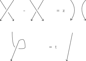
Figure 1.

It is easy to follow that the removal an unknot is equivalent to time a scalar $s=\frac{t-t^{-1}}{q-q^{-1}}$, i.e we have the relation showed in Figure 2.

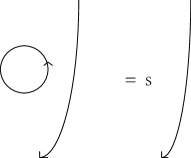
Figure 2.

2.1. The plane

When $F=\mathbb{R}^{2}$, it is easy to follow that every element in $\mathcal{S}(F)$ can be represented as a scalar in $\Lambda$. For a link $\mathcal{L}$ with a diagram $D_{\mathcal{L}}$, the resulting scalar $\langle D_{\mathcal{L}}\rangle\in\Lambda$ is the framed HOMFLYPT polynomial of the link $\mathcal{L}$. In the following, we will also use the notation $\langle\mathcal{L}\rangle$ to denote the $\langle D_{\mathcal{L}}\rangle$ for simplicity. In particular, as to the unknot $U$, we have $\langle U\rangle=\frac{t-t^{-1}}{q-q^{-1}}$.

The classical HOMFLYPT polynomial is defined by

(2.1) $$P_{\mathcal{L}}(q,t)=\frac{t^{-w(\mathcal{L})}\langle\mathcal{L}\rangle}{\langle U\rangle},$$

where $w(\mathcal{L})$ is the writhe number of the link $\mathcal{L}$. Particularly, $P_{U}(q,t)=1$.

Remark 2.1.

In some physical literatures, such as [16], the self-writhe $\bar{w}(\mathcal{L})$ instead of $w(\mathcal{L})$ is used in the definition of the HOMFLYPT polynomial (2.1). The relationship between them is

(2.2) $$w(\mathcal{L})=\bar{w}(\mathcal{L})+2lk(\mathcal{L}),$$

where $lk(\mathcal{L})$ is the total linking number of the link $\mathcal{L}$. By definition $\bar{w}(\mathcal{L})=\sum_{\alpha=1}^{L}w(\mathcal{K}_{\alpha})$, if $\mathcal{L}$ is a link with $L$ components $\mathcal{K}_{\alpha}$, $\alpha=1,...,L$.

2.2. The rectangle

We write $H_{n,m}(q,t)$ for the skein $\mathcal{S}(F)$ of $(n,m)$-tangle where $F$ is the rectangle with $n$ inputs and $m$ outputs at the top and matching inputs and outputs at the bottom. There is a natural algebra structure on $H_{n,m}$ by placing tangles one above the another. When $m=0$, we write $H_{n}(q,t)=H_{n,0}(q,t)$.

The algebra $H_{n,m}^{N}(q)$ is a generalization of the Iwahori-Hecke algebra of type $A$ constructed in [8].

Definition 2.2.

For integers $n,m\geq 0$ and $N\geq n+m$, we define $H^{N}_{n,m}(q)$ to be the associative $\mathbb{C}(q)$-algebra with unit presented by generators $g_{1},g_{2},\cdots,g_{n-1}$, $e$ (if $m=1$), $g_{1}^{*},g_{2}^{*},\cdots,g_{m-1}^{*}$ (if $m\geq 2$) and the relations:

(1) $g_{i}g_{j}=g_{j}g_{i}$,  $1\leq i,j\leq n-1,|i-j|\geq 2$;

(2) $g_{i}g_{i+1}g_{i}=g_{i+1}g_{i}g_{i+1}$,  $1\leq i\leq n-2$;

(3) $(g_{i}-q)(g_{i}+q^{-1})=0$,  $1\leq i\leq n-1$;

(4) $g_{i}^{*}g_{j}^{*}=g_{j}^{*}g_{i}^{*}$,  $1\leq i,j\leq m-1,|i-j|\geq 2$;

(5) $g_{i}^{*}g_{i+1}^{*}g_{i}^{*}=g_{i+1}^{*}g_{i}^{*}g_{i+1}^{*}$,  $1\leq i\leq m-2$;

(6) $(g_{i}^{*}-q)(g_{i}^{*}+q^{-1})=0$,  $1\leq i\leq m-1$;

(7) $e^{2}=[N]e$;

(8) $eg_{i}=g_{i}e$,  $1\leq i\leq n-2$;

(9) $eg_{i}^{*}=g_{i}^{*}e$,  $2\leq i\leq m-1$;

(10) $g_{i}g_{j}^{*}=g_{j}^{*}g_{i}$,  $1\leq i\leq n-1,1\leq j\leq m-1$;

(11) $eg_{n-1}e=q^{N}e$;

(12) $eg_{1}^{*}e=q^{N}e$;

(13) $eg_{n-1}^{-1}g_{1}^{*}e(g_{n-1}-g_{1}^{*})=0$;

(14) $(g_{n-1}-g_{1}^{*})eg_{n-1}^{-1}g_{1}^{*}e=0$.

If we take $t=q^{N}$, the skein $H_{n,m}(q,q^{N})\cong H_{n,m}^{N}(q)$.

2.3. The annulus

Let $\mathcal{C}$ be the HOMFLY skein of the annulus, i.e. $\mathcal{C}=\mathcal{S}(S^{1}\otimes I)$. $\mathcal{C}$ is a commutative algebra with the product induced by placing one annulus outside another. Let $T\in H_{n,m}$ be a $(n,m)$-tangle, we denote by $\hat{T}$ its closure in the annulus. This is a $\Lambda$-linear map, whose image we write $\mathcal{C}_{n,m}$. It is clear that every diagram in the annulus presents an elements in some $\mathcal{C}_{n,m}$.

As an algebra, $\mathcal{C}$ is freely generated by the set $\{A_{m}:m\in\mathbb{Z}\}$, $A_{m}$ for $m\neq 0$ is the closure of the braid $\sigma_{|m|-1}\cdots\sigma_{2}\sigma_{1}$, and $A_{0}$ is the empty diagram [23]. It follows that $\mathcal{C}$ contains two subalgebras $\mathcal{C}_{+}$ and $\mathcal{C}_{-}$ which are generated by $\{A_{m}:m\in\mathbb{Z},m\geq 0\}$ and $\{A_{m}:m\in\mathbb{Z},m\leq 0\}$. The algebra $\mathcal{C}_{+}$ is spanned by the subspace $\mathcal{C}_{n,0}$. There is a good basis $\{Q_{\lambda}\}$ of $\mathcal{C}_{+}$ consisting of the closures of certain idempotents of Hecke algebra $H_{n,0}(q,t)$.

In [5], R. Hadji and H. Morton constructed the basis elements $\{Q_{\lambda,\mu}\}$ explicitly for $\mathcal{C}$. We will review this construction in next section.

2.4. Skein involutions

For every surface $F$, first we can define the mirror map $\bar{\quad}$: $\mathcal{S}(F)\rightarrow\mathcal{S}(F)$ as follows. For a tangle $T$, we define the mirror $\bar{T}$ to be $T$ with all its crossings switched. For the coefficient ring $\Lambda$, we define the mirror by $\bar{q}=q^{-1},\ \bar{t}=t^{-1}$.

For the annulus $S^{1}\times I$, rotation the diagrams in $S^{1}\times I$ by $\pi$ about the horizontal axis through the center of annulus induces a map $*:\mathcal{C}\rightarrow\mathcal{C}$. It is easy to see that $(A_{m})^{*}=A_{-m}$, $(\mathcal{C}_{+})^{*}=\mathcal{C}_{-}$ and $(\mathcal{C}_{n,m})^{*}=\mathcal{C}_{m,n}$.

3. Full colored HOMFLYPT invariants

3.1. Partitions and symmetric functions

A partition $\lambda$ is a finite sequence of positive integers $(\lambda_{1},\lambda_{2},..)$ such that

(3.1) $$\lambda_{1}\geq\lambda_{2}\geq\cdots$$

The length of $\lambda$ is the total number of parts in $\lambda$ and denoted by $l(\lambda)$. The degree of $\lambda$ is defined by

(3.2) $$|\lambda|=\sum_{i=1}^{l(\lambda)}\lambda_{i}.$$

If $|\lambda|=d$, we say $\lambda$ is a partition of $d$ and denoted as $\lambda\vdash d$. The automorphism group of $\lambda$, denoted by Aut($\lambda$), contains all the permutations that permute parts of $\lambda$ by keeping it as a partition. Obviously, Aut($\lambda$) has the order

(3.3) $$|\text{Aut}(\lambda)|=\prod_{i=1}^{l(\lambda)}m_{i}(\lambda)!$$

where $m_{i}(\lambda)$ denotes the number of times that $i$ occurs in $\lambda$. We can also write a partition $\lambda$ as

(3.4) $$\lambda=(1^{m_{1}(\lambda)}2^{m_{2}(\lambda)}\cdots).$$

Every partition can be identified as a Young diagram. The Young diagram of $\lambda$ is a graph with $\lambda_{i}$ boxes on the $i$-th row for $j=1,2,..,l(\lambda)$, where we have enumerate the rows from top to bottom and the columns from left to right.

Given a partition $\lambda$, we define the conjugate partition $\lambda^{t}$ whose Young diagram is the transposed Young diagram of $\lambda$ which is derived from the Young diagram of $\lambda$ by reflection in the main diagonal.

Denote by $\mathcal{P}$ the set of all partitions. We define the $n$-th Cartesian product of $\mathcal{P}$ as $\mathcal{P}^{n}=\mathcal{P}\times\cdots\times\mathcal{P}$. The elements in $\mathcal{P}^{n}$ denoted by $\vec{A}=(A^{1},..,A^{n})$ are called partition vectors.

The following numbers associated with a given partition $\lambda$ are used frequently in this paper:

(3.5) $$z_{\lambda} =\prod_{j=1}^{l(\lambda)}j^{m_{j}(\lambda)}m_{j}(\lambda)!,$$

(3.6) $$k_{\lambda} =\sum_{j=1}^{l(\lambda)}\lambda_{j}(\lambda_{j}-2j+1).$$

Obviously, $k_{\lambda}$ is an even number and $k_{\lambda}=-k_{\lambda^{t}}$.

The $m$-th complete symmetric function $h_{m}$ is defined by its generating function

(3.7) $$H(t)=\sum_{m\geq 0}h_{m}t^{m}=\prod_{i\geq 1}\frac{1}{(1-x_{i}t)}.$$

The $m$-th elementary symmetric function $e_{m}$ is defined by its generating function

(3.8) $$E(t)=\sum_{m\geq 0}e_{m}t^{m}=\prod_{i\geq 1}(1+x_{i}t).$$

Obviously,

(3.9) $$H(t)E(-t)=1.$$

The power sum symmetric function of infinite variables $x=(x_{1},..,x_{N},..)$ is defined by

(3.10) $$p_{n}(x)=\sum_{i}x_{i}^{n}.$$

Given a partition $\lambda$, define

(3.11) $$p_{\lambda}(x)=\prod_{j=1}^{l(\lambda)}p_{\lambda_{j}}(x).$$

The Schur function $s_{\lambda}(x)$ is determined by the Frobenius formula

(3.12) $$s_{\lambda}(x)=\sum_{|\mu|=|\lambda|}\frac{\chi_{\lambda}(C_{\mu})}{z_{\mu}}p_{\mu}(x).$$

where $\chi_{\lambda}$ is the character of the irreducible representation of the symmetric group $S_{|\mu|}$ corresponding to $\lambda$. $C_{\mu}$ denotes the conjugate class of symmetric group $S_{|\mu|}$ corresponding to partition $\mu$. The orthogonality of character formula gives

(3.13) $$\sum_{A}\frac{\chi_{A}(C_{\mu})\chi_{A}(C_{\nu})}{z_{\mu}}=\delta_{\mu\nu}.$$

For $\lambda,\mu,\nu\in\mathcal{P}$, we define the littlewood-Richardson coefficient $c_{\lambda,\mu}^{\nu}$ as

(3.14) $$s_{\lambda}(x)s_{\mu}(x)=\sum_{\nu}c_{\lambda,\mu}^{\nu}s_{\nu}(x).$$

It is easy to see that $c_{\lambda,\mu}^{\nu}$ can be expressed by the characters of symmetric group by using the Frobenius formula

(3.15) $$c_{\lambda,\mu}^{\nu}=\sum_{\rho,\tau}\frac{\chi_{\lambda}(C_{\rho})}{z_{\rho}}\frac{\chi_{\lambda}(C_{\tau})}{z_{\tau}}\chi_{\nu}(C_{\rho\cup\tau}).$$

3.2. Basic elements in $\mathcal{C}$

Given a permutation $\pi\in S_{m}$ with the length $l(\pi)$, let $\omega_{\pi}$ be the positive permutation braid associated to $\pi$. We have $l(\pi)=w(\omega_{\pi})$, the writhe number of the braid $\omega_{\pi}$.

We define the quasi-idempotent element in $H_{m}$:

(3.16) $$a_{m}=\sum_{\pi\in S_{m}}q^{l(\pi)}\omega_{\pi}$$

Let element $h_{m}\in\mathcal{C}_{m,0}$ be the closure of the elements $\frac{1}{\alpha_{m}}a_{m}\in H_{m}$, i.e $h_{m}=\frac{1}{\alpha_{m}}\hat{a}_{m}$. Where $\alpha_{m}$ is determined by the equation $a_{m}a_{m}=\alpha_{m}a_{m}$, it gives $\alpha_{m}=q^{m(m-1)/2}\prod_{i=1}^{m}\frac{q^{i}-q^{-i}}{q-q^{-1}}$.

The skein $\mathcal{C}_{+}$ ($\mathcal{C}_{-}$) is spanned by the monomials in $\{h_{m}\}_{m\geq 0}$ ($\{h_{k}^{*}\}_{k\geq 0}$). The whole skein $\mathcal{C}$ is spanned by the monomials in $\{h_{m},h_{k}^{*}\}_{m,k\geq 0}$. $\mathcal{C}_{+}$ can be regarded as the ring of symmetric functions in variables $x_{1},..,x_{N},..$ with the coefficient ring $\Lambda$. In this situation, $\mathcal{C}_{m,0}$ consists of the homogeneous functions of degree $m$. The power sum $P_{m}=\sum x_{i}^{m}$ are symmetric functions which can be represented in terms of the complete symmetric functions, hence $P_{m}\in\mathcal{C}_{m,0}$. Moreover, we have the identity

(3.17) $$\{m\}P_{m}=X_{m}=\sum_{j=0}^{m-1}A_{m-1-j,j}.$$

where $\{m\}=\frac{q^{m}-q^{-m}}{q-q^{-1}}$ and $A_{i,j}$ is the closure of the braid $\sigma_{i+j}\sigma_{i+j-1}\cdots\sigma_{j+1}\sigma_{j}^{-1}\cdots\sigma_{1}^{-1}$. Given a partition $\mu$, we define

(3.18) $$P_{\mu}=\prod_{i=1}^{l(\mu)}P_{\mu_{i}}.$$

3.3. The meridian maps of $\mathcal{C}$

Take a diagram $X$ in the annulus and link it once with a simple meridian loop, oriented in either direction, to give diagrams $\varphi(X)$ and $\bar{\varphi}(x)$ in the annulus. This induces linear endmorphisms $\varphi,\bar{\varphi}$ of the skein $\mathcal{C}$, called the meridian maps. Each space $\mathcal{C}_{n,m}$ is invariant under $\varphi$ and $\bar{\varphi}$ [17].

It is showed in [13] that the eigenvectors of $\varphi$ on $\mathcal{C}_{n,0}$ are identified with $Q_{\lambda}$, the closure of the idempotents in Hecke algebra $H_{n}$. Moreover, $Q_{\lambda}$ can be expressed as explicit integer polynomials in $\{h_{m}\}_{m\geq 0}$. Then, in [5], Hadji and Morton constructed the eigenvectors of $\varphi$ on the whole skein $\mathcal{C}$ as follow.

3.4. Construction of the elements $Q_{\lambda,\mu}$

Given two partitions $\lambda,\mu$ with $l$ and $r$ parts. We first construct a $(l+r)\times(l+r)$-matrix $M_{\lambda,\mu}$ with entries in $\{h_{m},h_{k}^{*}\}_{m,k\in\mathbb{Z}}$ as follows, where we have let $h_{m}=0$, if $m<0$ and $h_{k}^{*}=0$ if $k<0$.

(3.19) $$M_{\lambda,\mu}=\begin{pmatrix}h_{\mu_{r}}^{*}&h_{\mu_{r}-1}^{*}&\cdots&h_{\mu_{r}-r-l+1}^{*}\\ h_{\mu_{r-1}+1}^{*}&h_{\mu_{r-1}}^{*}&\cdots&h_{\mu_{r-1}-r-l}^{*}\\ \cdot&\cdot&\cdots&\cdot\\ h_{\mu_{1}+(r-1)}^{*}&h_{\mu_{1}+(r-2)}^{*}&\cdots&h_{\mu_{1}-l}^{*}\\ h_{\lambda_{1}-r}&h_{\lambda_{1}-(r-1)}&\cdots&h_{\lambda_{1}+l-1}\\ \cdot&\cdot&\cdots&\cdot\\ h_{\lambda_{l}-l-r+1}&h_{\lambda_{l}-s-r+2}&\cdots&h_{\lambda_{l}}\end{pmatrix}$$

It is easy to note that the subscripts of the diagonal entries in the $h$-rows are the parts $\lambda_{1},\lambda_{2},...,\lambda_{l}$ of $\lambda$ in order, while the subscripts of the diagonal entries in the $h^{*}$-rows are the parts $\mu_{1},\mu_{2},..,\mu_{r}$ of $\mu$ in reverse order.

Then, $Q_{\lambda,\mu}$ is defined as the determinant of the matrix $M_{\lambda,\mu}$.

(3.20) $$Q_{\lambda,\mu}=\det M_{\lambda,\mu}.$$

Example 3.1.

For two partitions $\lambda=(4,2,2)$ and $\mu=(3,2)$. Then

(3.21) $$Q_{\lambda,\mu}=\det\begin{pmatrix}h_{2}^{*}&h_{1}^{*}&1&0&0\\ h_{4}^{*}&h_{3}^{*}&h_{2}^{*}&h_{1}^{*}&1\\ h_{2}&h_{3}&h_{4}&h_{5}&h_{6}\\ 0&1&h_{1}&h_{2}&h_{3}\\ 0&0&1&h_{1}&h_{2}\end{pmatrix}.$$

Given two partitions $\lambda,\mu$, define

(3.22) $$k_{\lambda,\mu}=(q-q^{-1})\left(t\sum_{x\in\lambda}q^{2c(x)}-t^{-1}\sum_{x\in\mu}q^{-2c(x)}\right)+\frac{t-t^{-1}}{q-q^{-1}}$$

where $c(x)=j-i$ is the content of the cell in row $i$ and column $j$ of the diagram. It is showed in [17] that the set $k_{\lambda,\mu}$ forms a complete set of eigenvalues of the meridian map $\varphi$, each occurring with multiplicity $1$. Furthermore, it is prove in [5] that the element $Q_{\lambda,\mu}$ is an eigenvector of the meridian map $\varphi$, with eigenvalue $k_{\lambda,\mu}$. Thus $\{Q_{\lambda,\mu}\}$ forms a basis of $\mathcal{C}$. Moreover, the basis elements $Q_{\lambda,\mu}$ of $\mathcal{C}$ have the property that the product of any two is a non-negative integer linear combination of basis elements.

(3.23) $$Q_{\lambda,\mu}=\sum_{\sigma,\rho,\nu}(-1)^{|\sigma|}c_{\sigma,\rho}^{\lambda}c_{\sigma^{t},\nu}^{\mu}Q_{\rho,\emptyset}Q_{\emptyset,\nu}.$$

3.5. Full colored HOMFLYPT invariants

Let $\mathcal{L}$ be a framed link with $L$ components with a fixed numbering. For diagrams $Q_{1},..,Q_{L}$ in the skein model of annulus with the positive oriented core $\mathcal{C}^{+}$, we define the decoration of $\mathcal{L}$ with $Q_{1},..,Q_{L}$ as the link

(3.24) $$\mathcal{L}\star\otimes_{\alpha=1}^{L}Q_{\alpha}$$

which derived from $\mathcal{L}$ by replacing every annulus $\mathcal{L}$ by the annulus with the diagram $Q_{\alpha}$ such that the orientations of the cores match. Each $Q_{\alpha}$ has a small backboard neighborhood in the annulus which makes the decorated link $\mathcal{L}\otimes_{\alpha=1}^{L}Q_{\alpha}$ into a framed link.

In particular, when $Q_{\lambda^{\alpha},\mu^{\alpha}}\in\mathcal{C}_{d_{\alpha},t_{\alpha}}$, where $\lambda^{\alpha},\mu^{\alpha}$ are the partitions of positive integers $d_{\alpha}$ and $t_{\alpha}$ respectively, for $\alpha=1,..,L$.

Definition 3.2.

The framed full colored HOMFLYPT invariant $\mathcal{H}(\mathcal{L};\otimes_{\alpha=1}^{L}Q_{\lambda^{\alpha},\mu^{\alpha}})$ of $\mathcal{L}$ is defined to be the HOMFLYPT polynomial (framing-dependence) of the decorated link $\mathcal{L}\star\otimes_{\alpha=1}^{L}Q_{\lambda^{\alpha},\mu^{\alpha}}$, i.e. $\mathcal{H}(\mathcal{L};\otimes_{\alpha=1}^{L}Q_{\lambda^{\alpha},\mu^{\alpha}})=\langle\mathcal{L}\star\otimes_{\alpha=1}^{L}Q_{\lambda^{\alpha},\mu^{\alpha}}\rangle$.

By the result in [3], it is easy to show that the framing factor for $Q_{\lambda,\mu}$ is $q^{\kappa_{\lambda}+\kappa_{\mu}}t^{|\lambda|+|\mu|}$.

Definition 3.3.

The (framing-independence) full colored HOMFLYPT invariant of $\mathcal{L}$ is defined as follow:

(3.25) $$W_{[\lambda^{1},\mu^{1}],[\lambda^{2},\mu^{2}],..,[\lambda^{L},\mu^{L}]}(\mathcal{L})$$

$$=q^{-\sum_{\alpha=1}^{L}(\kappa_{\lambda^{\alpha}}+\kappa_{\mu^{\alpha}})w(\mathcal{K}_{\alpha})}t^{-\sum_{\alpha=1}^{L}(|\lambda^{\alpha}|+|\mu^{\alpha}|)w(\mathcal{K}_{\alpha})}\langle\mathcal{L}\star\otimes_{\alpha=1}^{L}Q_{\lambda^{\alpha},\mu^{\alpha}}\rangle.$$

In particular, when $\mu^{\alpha}=\emptyset$, for $\alpha=1,...,L$. Then $W_{[\lambda^{1},\emptyset],..,[\lambda^{L},\emptyset]}(\mathcal{L})$ is reduced to the original colored HOMFLYPT invariant $W_{\vec{\lambda}}(\mathcal{L})$ defined in [26].

Example 3.4.

For the unknot $U$, by the formula (3.23), we have

(3.26) $$W_{[\lambda,\nu]}(U)=\langle Q_{\lambda,\mu}\rangle=\sum_{\sigma,\rho,\nu}(-1)^{|\sigma|}c_{\sigma,\rho}^{\lambda}c_{\sigma^{t},\nu}^{\mu}s_{\rho}^{\#}(q,t)s_{\nu}^{\#}(q,t).$$

where $s_{\mu}^{\#}(q,t)$ denotes the colored HOMFLYPT invariant $W_{\mu}(U)$ of $U$.

Throughout this paper, we use the notation $s_{\lambda,\nu}^{\#}(q,t)$ to denote the full colored HOMFLYPT invariant of the unknot $W_{[\lambda,\nu]}(U)$.

3.6. Symmetric properties

By the definition the mirror map $\bar{\quad}$ and $*$ map, it is easy to see

(3.27) $$\overline{Q_{\lambda,\mu}}=Q_{\lambda,\mu},\ Q_{\lambda,\mu}^{*}=Q_{\mu,\lambda}.$$

For a knot $\mathcal{K}$, we have

(3.28) $$\mathcal{H}(\mathcal{K};Q_{\lambda,\mu})=\mathcal{H}(\mathcal{K};Q_{\mu,\lambda}^{*})=\mathcal{H}(\mathcal{K};Q_{\mu,\lambda}).$$

where the last equality is followed by the fact that the HOMFLYPT polynomial of a knot is independent of its orientation. For a link $\mathcal{L}$ with $L$-components, we have

(3.29) $$\mathcal{H}(\mathcal{L};\otimes_{\alpha=1}^{L}Q_{\lambda^{\alpha},\mu^{\alpha}})=\mathcal{H}(\mathcal{L};\otimes_{\alpha=1}^{L}Q_{\mu^{\alpha},\lambda^{\alpha}}^{*})=\mathcal{H}(\mathcal{L};\otimes_{\alpha=1}^{L}Q_{\mu^{\alpha},\lambda^{\alpha}}).$$

Given a partition $\lambda$, let $\lambda^{t}$ be its conjugate partition. Then in the skein $\mathcal{C}$ we have

(3.30) $$Q_{\lambda,\mu}|_{q\rightarrow-q^{-1}}=Q_{\lambda^{t},\mu^{t}}.$$

Therefore, for a link $\mathcal{L}$, we have

(3.31) $$\mathcal{H}(\mathcal{L};\otimes_{\alpha=1}^{L}Q_{\lambda^{\alpha},\mu^{\alpha}};q,t)=\mathcal{H}(\mathcal{L};\otimes_{\alpha=1}^{L}Q_{(\lambda^{\alpha})^{t},(\mu^{\alpha})^{t}};-q^{-1},t).$$

4. Full colored HOMFLYPT invariants for torus links

Let us consider the $L$-component torus link $T=T_{mL}^{nL}$ which is the closure of the framed $mL$-braid $(\beta_{mL})^{nL}$, where $(m,n)=1$. The braid $\beta_{m}$ is showed in Figure 3.

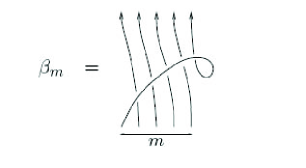
Figure 3.

Remark 4.1.

In some literatures (such as [14]), the $L$-component torus link $T(mL,nL)$ is defined to be the closure of the braid $(\sigma_{1}\cdots\sigma_{mL-1})^{nL}$. It is clear that $T_{mL}^{nL}$ and $T(mL,nL)$ represent the same torus link but with different framings.

$T=T_{mL}^{nL}$ induces a map $F_{mL}^{nL}:\otimes_{\alpha=1}^{L}\mathcal{C}_{d_{\alpha},r_{\alpha}}\rightarrow\mathcal{C}_{m(\sum_{\alpha=1}^{L}d_{\alpha}),m(\sum_{\alpha=1}^{L}r_{\alpha})}$ by taking an element $\otimes_{\alpha=1}^{L}Q_{\lambda^{\alpha},\mu^{\alpha}}$ to $T_{mL}^{nL}\star\otimes_{\alpha=1}^{L}Q_{\lambda^{\alpha},\mu^{\alpha}}$. We define $\tau=F^{1}_{1}$, then $\tau$ is the framing change map. Thus if we let

(4.1) $$\tau(Q_{\lambda,\mu})=\tau_{\lambda,\mu}Q_{\lambda,\mu}$$

then $\tau_{\lambda,\mu}=q^{\kappa_{\lambda}+\kappa_{\mu}}t^{|\lambda|+|\mu|}$. We define the fractional twist map $\tau^{\frac{n}{m}}:\mathcal{C}\rightarrow\mathcal{C}$ as the linear map on the basis $Q_{\lambda,\mu}$ given by

(4.2) $$\tau^{\frac{n}{m}}(Q_{\lambda,\mu})=(\tau_{\lambda,\mu})^{\frac{n}{m}}Q_{\lambda,\mu}.$$

In the following, we give an explicit expression for $F^{nL}_{mL}(\otimes_{\alpha=1}^{L}Q_{\lambda^{\alpha},\mu^{\alpha}})$. Let $\Lambda_{x}$ and $\Lambda_{x^{*}}$ be the rings of symmetric functions with variables $(x_{1},x_{2},....)$ and $(x_{1}^{*},x_{2}^{*},...)$ respectively. The Schur functions $s_{\lambda}(x)(\lambda\in\mathcal{P})$ forms a basis of the ring $\Lambda_{x}$ [15]. It is showed in [9] that the polynomials $s_{\lambda,\mu}(x;x^{*})(\lambda,\mu\in\mathcal{P})$ (the notation $[\lambda,\mu]_{GL}$ in [9]) forms a $\mathbb{Z}$ basis of the ring $\Lambda_{x}\otimes\Lambda_{x^{*}}$. We define the $m$-th Adams operator $\Psi_{m}$ on $\Lambda_{x}$ and $\Lambda_{x}\otimes\Lambda_{x^{*}}$ as follow:

(4.3) $$\Psi_{m}(s_{\lambda}(x))=s_{\lambda}(x^{m}),\ \Psi_{m}(s_{\lambda,\mu}(x;x^{*}))=s_{\lambda,\mu}(x^{m};x^{*m}).$$

Since $\mathcal{C}_{+}$ is isomorphic to the ring $\Lambda_{x}$. $\mathcal{C}$ is isomorphic to the ring $\Lambda_{x}\otimes\Lambda_{x^{*}}$. For any $Q\in\mathcal{C}_{d,r}$, $\Psi_{m}(Q)$ is well-defined. Moreover, $\Psi_{m}(Q)\in\mathcal{C}_{md,mr}$.

We have the following formula which is the generalization of Theorem 13 showed in [18]

(4.4) $$F_{mL}^{nL}(\otimes_{\alpha=1}^{L}Q_{\lambda^{\alpha},\mu^{\alpha}})=\tau^{\frac{n}{m}}(\prod_{\alpha=1}^{L}\Psi_{m}(Q_{\lambda^{\alpha},\mu^{\alpha}})).$$

Since $\{Q_{\lambda,\mu}:\lambda,\mu\in\mathcal{P},|\lambda|=d,|\mu|=r\}$ forms a basis of $\mathcal{C}_{d,r}$, we have the expansion

(4.5) $$\prod_{\alpha=1}^{L}\Psi_{m}(Q_{\lambda^{\alpha},\mu^{\alpha}})=\sum_{\rho,\nu}C_{[\lambda^{1},\mu^{1}],..,[\lambda^{L},\mu^{L}];m}^{[\rho,\nu]}Q_{\rho,\nu},$$

where $C_{[\lambda^{1},\mu^{1}],..,[\lambda^{L},\mu^{L}];m}^{[\rho,\nu]}$ are the coefficients given by the following formula

(4.6) $$\prod_{\alpha=1}^{L}\Psi_{m}(s_{\lambda^{\alpha},\mu^{\alpha}}(x;x^{*}))=\sum_{\rho,\nu}C_{[\lambda^{1},\mu^{1}],..,[\lambda^{L},\mu^{L}];m}^{[\rho,\nu]}s_{\rho,\nu}(x;x^{*}).$$

By the definition of the fractional twist map of $\tau^{\frac{n}{m}}$, we obtain

(4.7) $$F_{mL}^{nL}(\otimes_{\alpha=1}^{L}Q_{\lambda^{\alpha},\mu^{\alpha}})=\sum_{\rho,\nu}C_{[\lambda^{1},\mu^{1}],..,[\lambda^{L},\mu^{L}];m}^{[\rho,\nu]}q^{\frac{n}{m}(\kappa_{\rho}+\kappa_{\nu})}t^{\frac{n}{m}(|\rho|+|\nu|)}Q_{\rho,\nu}.$$

Therefore, by Definition 3.3, the full colored HOMFLYPT invariants of the torus link $T_{mL}^{nL}$ is given by

(4.8) $$W_{[\lambda^{1},\mu^{1}],..,[\lambda^{L},\mu^{L}]}(T_{mL}^{nL})$$

$$=q^{-m\cdot n\sum_{\alpha=1}^{L}(\kappa_{\lambda^{\alpha}}+\kappa_{\mu^{\alpha}})}t^{-n\cdot m\sum_{\alpha=1}^{L}(|\lambda^{\alpha}|+|\mu^{\alpha}|)}\langle F_{mL}^{nL}(\otimes_{\alpha=1}^{L}Q_{\lambda^{\alpha},\mu^{\alpha}})\rangle$$

$$=q^{-m\cdot n\sum_{\alpha=1}^{L}(\kappa_{\lambda^{\alpha}}+\kappa_{\mu^{\alpha}})}t^{-n\cdot m\sum_{\alpha=1}^{L}(|\lambda^{\alpha}|+|\mu^{\alpha}|)}$$

$$\sum_{\rho,\nu}C_{[\lambda^{1},\mu^{1}],..,[\lambda^{L},\mu^{L}];m}^{[\rho,\nu]}q^{\frac{n}{m}(\kappa_{\rho}+\kappa_{\nu})}t^{\frac{n}{m}(|\rho|+|\nu|)}\langle Q_{\rho,\nu}\rangle.$$

where $\langle Q_{\rho,\nu}\rangle=s^{\#}_{\rho,\nu}(q,t)$ is the full colored HOMFLYPT invariant of the unknot $U$.

Now, let us give the explicit expression of the coefficient $C_{[\lambda^{1},\mu^{1}],..,[\lambda^{L},\mu^{L}];m}^{[\rho,\nu]}$. We need the following formulas in [9].

(4.9) $$s_{\xi,\eta}(x;x^{*})s_{\rho,\nu}(x;x^{*})=M_{[\xi,\eta],[\rho,\nu]}^{[\lambda,\mu]}s_{\lambda,\mu}(x;x^{*}),$$

where

(4.10) $$M_{[\xi,\eta],[\rho,\nu]}^{[\lambda,\mu]}=\sum_{\beta,\gamma,\theta,\delta}\left(\sum_{\sigma}c_{\sigma,\beta}^{\xi}c_{\sigma,\gamma}^{\nu}\right)\left(\sum_{\epsilon}c_{\epsilon,\theta}^{\eta}c_{\epsilon,\delta}^{\rho}\right)c_{\beta,\delta}^{\lambda}c_{\gamma,\theta}^{\mu}.$$

(4.11) $$s_{\lambda,\mu}(x;x^{*})=\sum_{\sigma,\rho,\nu}(-1)^{|\sigma|}c_{\sigma,\rho}^{\lambda}c_{\sigma^{t},\nu}^{\mu}s_{\rho}(x)s_{\nu}(x^{*}).$$

(4.12) $$s_{\lambda}(x)s_{\mu}(x^{*})=\sum_{\epsilon,\rho,\nu}c_{\epsilon,\rho}^{\lambda}c_{\epsilon,\nu}^{\mu}s_{\rho,\nu}(x;x^{*}).$$

Let $C_{\lambda;m}^{\rho}$ and $C_{[\lambda,\mu];m}^{[\rho,\nu]}$ be the coefficients determined by the following formulas:

(4.13) $$\Psi_{m}(s_{\lambda}(x))=\sum_{\rho}C_{\lambda;m}^{\rho}s_{\rho}(x),\ \Psi_{m}(s_{\lambda,\mu}(x;x^{*}))=\sum_{\rho,\nu}C_{[\lambda,\mu];m}^{[\rho,\nu]}s_{\rho,\nu}(x;x^{*}).$$

By formula (4.11), we have

(4.14) $$\Psi_{m}(s_{\lambda,\mu}(x;x^{*})) =\sum_{\sigma,\rho,\nu}(-1)^{|\sigma|}c_{\sigma,\rho}^{\lambda}c_{\sigma^{t},\nu}^{\mu}\Psi_{m}(s_{\rho}(x))\Psi_{m}(s_{\nu}(x^{*}))$$

$$=\sum_{\sigma,\rho,\nu}(-1)^{|\sigma|}c_{\sigma,\rho}^{\lambda}c_{\sigma^{t},\nu}^{\mu}\sum_{\delta,\theta}C_{\rho;m}^{\delta}C_{\nu;m}^{\theta}s_{\delta}(x)s_{\theta}(x^{*})$$

$$=\sum_{\sigma,\rho,\nu}(-1)^{|\sigma|}c_{\sigma,\rho}^{\lambda}c_{\sigma^{t},\nu}^{\mu}\sum_{\delta,\theta}C_{\rho;m}^{\delta}C_{\nu;m}^{\theta}\sum_{\epsilon,\beta,\gamma}c_{\epsilon,\beta}^{\delta}c_{\epsilon,\gamma}^{\theta}s_{\beta,\gamma}(x;x^{*})$$

Hence, we obtain

(4.15) $$C_{[\lambda,\mu];m}^{[\beta,\gamma]}=\sum_{\sigma,\rho,\nu,\delta,\theta,\epsilon}(-1)^{|\sigma|}c_{\sigma,\rho}^{\lambda}c_{\sigma^{t},\nu}^{\mu}C_{\rho;m}^{\delta}C_{\nu;m}^{\theta}c_{\epsilon,\beta}^{\delta}c_{\epsilon,\gamma}^{\theta}.$$

Therefore, as to the torus knot $T_{m}^{n}$, the full HOMFLYPT invariant is given by

(4.16) $$W_{[\lambda,\mu]}(T_{m}^{n};q,t)$$

$$=q^{-m\cdot n(\kappa_{\lambda}+\kappa_{\mu})}t^{-n\cdot m(|\lambda|+|\mu|)}\sum_{\rho,\nu}C_{[\lambda,\mu];m}^{[\rho,\nu]}q^{\frac{n}{m}(\kappa_{\rho}+\kappa_{\nu})}t^{\frac{n}{m}(|\rho|+|\nu|)}s^{\#}_{\rho,\nu}(q,t).$$

Finally, by formula (4.9), we have

(4.17) $$\prod_{\alpha=1}^{L}\Psi_{m}(s_{\lambda^{\alpha},\mu^{\alpha}}(x;x^{*}))$$

$$=\sum_{\beta^{1},\gamma^{1}}M_{[\lambda^{1},\mu^{1}],[\lambda^{2},\mu^{2}]}^{[\beta^{1},\gamma^{1}]}\Psi_{m}(s_{\beta^{1},\gamma^{1}}(x;x^{*}))\prod_{\alpha=3}^{L}\Psi_{m}(s_{\lambda^{\alpha},\mu^{\alpha}}(x;x^{*}))$$

$$=\cdots$$

$$=\sum_{\beta^{\alpha},\gamma^{\alpha}}M_{[\lambda^{1},\mu^{1}],[\lambda^{2},\mu^{2}]}^{[\beta^{1},\gamma^{1}]}M_{[\beta^{1},\gamma^{1}],[\lambda^{3},\mu^{3}]}^{[\beta^{2},\gamma^{2}]}\cdots M_{[\beta^{L-2},\gamma^{L-2}],[\lambda^{L},\mu^{L}]}^{[\beta^{L-1},\gamma^{L-1}]}\Psi_{m}(s_{\beta^{L-1},\gamma^{L-1}}(x;x^{*}))$$

$$=\sum_{\beta^{\alpha},\gamma^{\alpha}}M_{[\lambda^{1},\mu^{1}],[\lambda^{2},\mu^{2}],...,[\lambda^{L},\mu^{L}]}^{[\beta^{L-1},\gamma^{L-1}]}C_{[\beta^{L-1},\gamma^{L-1}];m}^{[\rho,\nu]}s_{\rho,\nu}(x;x^{*}).$$

where we have let

(4.18) $$M_{[\lambda^{1},\mu^{1}],[\lambda^{2},\mu^{2}],...,[\lambda^{L},\mu^{L}]}^{[\beta^{L-1},\gamma^{L-1}]}=\sum_{\beta^{\alpha},\gamma^{\alpha},\alpha=1,..,L-2}M_{[\lambda^{1},\mu^{1}],[\lambda^{2},\mu^{2}]}^{[\beta^{1},\gamma^{1}]}M_{[\beta^{1},\gamma^{1}],[\lambda^{3},\mu^{3}]}^{[\beta^{2},\gamma^{2}]}\cdots M_{[\beta^{L-2},\gamma^{L-2}],[\lambda^{L},\mu^{L}]}^{[\beta^{L-1},\gamma^{L-1}]}$$

Thus, we obtain the following formula

(4.19) $$C_{[\lambda^{1},\mu^{1}],..,[\lambda^{L},\mu^{L}];m}^{[\rho,\nu]}=\sum_{\beta,\gamma}M_{[\lambda^{1},\mu^{1}],[\lambda^{2},\mu^{2}],...,[\lambda^{L},\mu^{L}]}^{[\beta,\gamma]}C_{[\beta,\gamma];m}^{[\rho,\nu]}.$$

Combing the formula (4.16), we get the expression for the full HOMFLYPT invariant for torus link $T_{mL}^{nL}$:

(4.20) $$W_{[\lambda^{1},\mu^{1}],..,[\lambda^{L},\mu^{L}]}(T_{mL}^{nL}) =q^{-nm\sum_{\alpha=1}^{L}(\kappa_{\lambda^{\alpha}}+\kappa_{\mu^{\alpha}})}t^{-nm\sum_{\alpha=1}^{L}(|\lambda^{\alpha}|+|\mu^{\alpha}|)}$$

$$\sum_{\beta,\gamma}M_{[\lambda^{1},\mu^{1}],...,[\lambda^{L},\mu^{L}]}^{[\beta,\gamma]}q^{nm(\kappa_{\beta}+\kappa_{\gamma})}t^{nm(|\beta|+|\gamma|)}W_{[\beta,\gamma]}(T_{m}^{n};q,t).$$

Since $W_{[\lambda^{1},\mu^{1}],..,[\lambda^{L},\mu^{L}]}(\mathcal{L})$ is a framing-independent invariant, we also have

(4.21) $$W_{[\lambda^{1},\mu^{1}],..,[\lambda^{L},\mu^{L}]}(T(mL,nL))=W_{[\lambda^{1},\mu^{1}],..,[\lambda^{L},\mu^{L}]}(T_{mL}^{nL}).$$

Example 4.2.

As to the torus knot $T(2,2k+1)$, we have

(4.22) $$W_{[(1),(1)]}(T(2,2k+1)) =t^{-8k-4}\left(1+q^{-4k-2}t^{4k+2}s_{(1^{2}),(1^{2})}^{\#}\right.$$

$$\left.-t^{4k+2}s_{(1^{2}),(2)}^{\#}-t^{4k+2}s_{(2),(1^{2})}^{\#}+q^{4k+2}t^{4k+2}s_{(2),(2)}^{\#}\right).$$

(4.23) $$W_{[(2),(1)]}(T(2,2k+1)) =q^{-8k-4}t^{-12k-6}\left(-q^{-2k-1}t^{2k+1}s_{(1^{2}),\emptyset}^{\#}+q^{2k+1}t^{2k+1}s_{(2),\emptyset}^{\#}\right.$$

$$\left.-q^{-2k-1}t^{6k+3}s_{(2^{2}),(1^{2})}^{\#}+q^{2k+1}t^{6k+3}s_{(2^{2}),(2)}^{\#}+q^{2k+1}t^{6k+3}s_{(31),(1^{2})}^{\#}\right.$$

$$\left.-q^{6k+3}t^{6k+3}s_{(31),(2)}^{\#}-q^{10k+5}t^{6k+3}s_{(4),(1^{2})}^{\#}+q^{14k+7}t^{6k+3}s_{(4),(2)}^{\#}\right).$$

(4.24) $$W_{[(1^{2}),(1)]}(T(2,2k+1)) =q^{8k+4}t^{-12k-6}\left(-q^{-2k-1}t^{2k+1}s_{(1^{2}),\emptyset}^{\#}+q^{2k+1}t^{2k+1}s_{(2),\emptyset}^{\#}\right.$$

$$\left.-q^{-14k-7}t^{6k+3}s_{(1^{4}),(1^{2})}^{\#}+q^{-10k-5}t^{6k+3}s_{(1^{4}),(2)}^{\#}+q^{-6k-3}t^{6k+3}s_{(21^{2}),(1^{2})}^{\#}\right.$$

$$\left.-q^{-2k-1}t^{6k+3}s_{(21^{2}),(2)}^{\#}-q^{-2k-1}t^{6k+3}s_{(2^{2}),(1^{2})}^{\#}+q^{2k+1}t^{6k+3}s_{(2^{2}),(2)}^{\#}\right).$$

(4.25) $$W_{[(1^{2}),(1^{2})]}(T(2,2k+1)) =q^{16k+8}t^{-16k-8}\left(1+q^{-4k-2}t^{4k+2}s_{(1^{2}),(1^{2})}^{\#}-t^{4k+2}s_{(1^{2}),(2)}^{\#}\right.$$

$$\left.-t^{4k+2}s_{(2),(1^{2})}^{\#}+q^{4k+2}t^{4k+2}s_{(2),(2)}^{\#}+q^{-24k-12}t^{8k+4}s_{(1^{4}),(1^{4})}^{\#}\right.$$

$$\left.-q^{-16k-8}t^{8k+4}s_{(1^{4}),(21^{2})}^{\#}+q^{-12k-6}t^{8k+4}s_{(1^{4}),(2^{2})}^{\#}\right.$$

$$\left.-q^{-16k-8}t^{8k+4}s_{(21^{2}),(1^{4})}^{\#}+q^{-8k-4}t^{8k+4}s_{(21^{2}),(21^{2})}^{\#}-q^{-4k-2}t^{8k+4}s_{(21^{2}),(2^{2})}^{\#}\right.$$

$$\left.+q^{-12k-6}t^{8k+4}s_{(2^{2}),(1^{4})}^{\#}-q^{-4k-2}t^{8k+4}s_{(2^{2}),(21^{2})}^{\#}+t^{8k+4}s_{(2^{2}),(2^{2})}^{\#}\right).$$

(4.26) $$W_{[(1^{2}),(2)]}(T(2,2k+1)) =t^{-16k-8}\left(q^{-4k-2}t^{4k+2}s_{(1^{2}),(1^{2})}^{\#}-t^{4k+2}s_{(1^{2}),(2)}^{\#}-t^{4k+2}s_{(2),(1^{2})}^{\#}\right.$$

$$\left.+q^{4k+2}t^{4k+2}s_{(2),(2)}^{\#}+q^{-12k-6}t^{8k+4}s_{(1^{4}),(2^{2})}^{\#}-q^{-8k-4}t^{8k+4}s_{(1^{4}),(31)}^{\#}\right.$$

$$\left.+t^{8k+4}s_{(1^{4}),(4)}^{\#}-q^{-4k-2}t^{8k+4}s_{(21^{2}),(2^{2})}^{\#}+t^{8k+4}s_{(21^{2}),(31)}^{\#}-q^{8k+4}t^{8k+4}s_{(21^{2}),(4)}^{\#}\right.$$

$$\left.+t^{8k+4}s_{(2^{2}),(2^{2})}^{\#}-q^{4k+2}t^{8k+4}s_{(2^{2}),(31)}^{\#}+q^{12k+6}t^{8k+4}s_{(2^{2}),(4)}^{\#}\right).$$

(4.27) $$W_{[(2),(2)]}(T(2,2k+1)) =q^{-16k-8}t^{-16k-8}\left(1+q^{-4k-2}t^{4k+2}s_{(1^{2}),(1^{2})}^{\#}-t^{4k+2}s_{(1^{2}),(2)}^{\#}\right.$$

$$\left.-t^{4k+2}s_{(2),(1^{2})}^{\#}+q^{4k+2}t^{4k+2}s_{(2),(2)}^{\#}+t^{8k+4}s_{(2^{2}),(2^{2})}^{\#}\right.$$

$$\left.-q^{4k+2}t^{8k+4}s_{(2^{2}),(31)}^{\#}+q^{12k+6}t^{8k+4}s_{(2^{2}),(4)}^{\#}-q^{4k+2}t^{8k+4}s_{(31),(2^{2})}^{\#}\right.$$

$$\left.+q^{8k+4}t^{8k+4}s_{(31),(31)}^{\#}-q^{16k+8}t^{8k+4}s_{(31),(4)}^{\#}+q^{12k+6}t^{8k+4}s_{(4),(2^{2})}^{\#}\right.$$

$$\left.-q^{16k+8}t^{8k+4}s_{(4),(31)}^{\#}+q^{24k+12}t^{8k+4}s_{(4),(4)}^{\#}\right).$$

5. Special polynomials

For a knot $\mathcal{K}$ and a partition $\lambda\in\mathcal{P}$, P. Dunin-Barkowski, A. Mironov, A. Morozov, A. Sleptsov and A. Smirnov [2] defined the following special polynomial

(5.1) $$H_{\lambda}^{\mathcal{K}}(t)=\lim_{q\rightarrow 1}\frac{W_{\lambda}(\mathcal{K};q,t)}{W_{\lambda}(U;q,t)}.$$

In particular, when $\lambda=(1)$, we have

(5.2) $$H_{(1)}^{\mathcal{K}}(t)=\lim_{q\rightarrow 1}\frac{W_{(1)}(\mathcal{K};q,t)}{W_{(1)}(U;q,t)}=P_{\mathcal{K}}(1,t)$$

where $P_{\mathcal{K}}(q,t)$ is the HOMFLYPT polynomial as defined in (2.1).

After testing many examples [2, 6, 7], they proposed the following conjectural formula:

(5.3) $$H_{\lambda}^{\mathcal{K}}(t)=H_{(1)}^{\mathcal{K}}(t)^{|\lambda|}.$$

A rigid mathematical proof of the formula (5.3) is given in [12] and [26] with different methods. In fact, they have proved that the formula (5.3) holds for any link $\mathcal{L}$. The special polynomial for a link $\mathcal{L}$ with $L$ components is defined as follow:

(5.4) $$H_{\vec{\lambda}}^{\mathcal{L}}(t)=\lim_{q\rightarrow 1}\frac{W_{\vec{\lambda}}(\mathcal{L};q,t)}{W_{\vec{\lambda}}(U^{\otimes L};q,t)}.$$

Theorem 5.1 ([12] and [26]).

Given $\vec{\lambda}=(\lambda^{1},..,\lambda^{L})\in\mathcal{P}^{L}$ and a link $\mathcal{L}$ with $L$ components $\mathcal{K}_{\alpha},\alpha=1,..,L$, then we have

(5.5) $$H_{\vec{\lambda}}^{\mathcal{L}}(t)=\prod_{\alpha=1}^{L}H_{(1)}^{\mathcal{K}_{\alpha}}(a)^{|\lambda^{\alpha}|}.$$

We can also define the special polynomial for full colored HOMFLYPT invariant for a link $\mathcal{L}$ with $L$ components similarly:

(5.6) $$H_{[\lambda^{1},\mu^{1}],..,[\lambda^{L},\mu^{L}]}^{\mathcal{L}}(t)=\lim_{q\rightarrow 1}\frac{W_{[\lambda^{1},\mu^{1}],..,[\lambda^{L},\mu^{L}]}(\mathcal{L};q,t)}{\prod_{\alpha=1}^{L}W_{[\lambda^{\alpha},\mu^{\alpha}]}(U;q,t)}.$$

Theorem 5.2.

For a link $\mathcal{L}$ with $L$ components $\mathcal{K}_{\alpha},\alpha=1,..,L$, we have

(5.7) $$H_{[\lambda^{1},\mu^{1}],..,[\lambda^{L},\mu^{L}]}^{\mathcal{L}}(t)=\prod_{\alpha=1}^{L}P_{\mathcal{K}_{\alpha}}(1,t)^{|\lambda^{\alpha}|+|\mu^{\alpha}|}.$$

In order to prove the Theorem 5.2, we need introduce a classical result due to Lichorish and Millet [10] which showed that for a given link $\mathcal{L}$ with $L$ components, the lowest power of $q-q^{-1}$ in the HOMFLYPT polynomial $P_{\mathcal{L}}(q,t)$ is $1-L$.

Theorem 5.3 (Lickorish-Millett [10]).

Let $\mathcal{L}$ be a link with $L$ components. The HOMFLYPT polynomial has the expansion

(5.8) $$P_{\mathcal{L}}(q,t)=\sum_{g\geq 0}p^{\mathcal{L}}_{2g+1-L}(t)(q-q^{-1})^{2g+1-L}$$

which satisfies

(5.9) $$p_{1-L}^{\mathcal{L}}(t)=t^{-2lk(\mathcal{L})}(t-t^{-1})^{L-1}\prod_{\alpha=1}^{L}p_{0}^{\mathcal{K}_{\alpha}}(t)$$

where $p_{0}^{\mathcal{K}_{\alpha}}(t)$ is the HOMFLYPT polynomial of the $\alpha$-th component of the link $\mathcal{L}$ with $q=1$, i.e. $p_{0}^{\mathcal{K}_{\alpha}}(t)=P_{\mathcal{K}_{\alpha}}(1,t)$.

By the definition in our notation (2.1), we have

(5.10) $$\langle\mathcal{L}\rangle=\sum_{g\geq 0}\hat{p}^{\mathcal{L}}_{2g+1-L}(t)(q-q^{-1})^{2g-L}$$

where $\hat{p}^{\mathcal{L}}_{2g+1-L}(t)=t^{w(\mathcal{L})}p^{\mathcal{L}}_{2g+1-L}(t)(t-t^{-1})$. Hence

(5.11) $$\hat{p}^{\mathcal{L}}_{1-L}(t)=t^{\bar{w}(\mathcal{L})}(t-t^{-1})^{L}\prod_{\alpha=1}^{L}p_{0}^{\mathcal{K}_{\alpha}}(t)$$

by the formula (2.2).

We now give the proof of the Theorem 5.2.

Proof.

We only give the proof for the case of a knot $\mathcal{K}$. It is easy to generalize the proof for any link $\mathcal{L}$. Given two partitions $\lambda$ and $\mu$ with $|\lambda|=n$ and $|\mu|=m$, since

(5.12) $$Q_{\lambda,\mu} =Q_{\lambda}Q_{\mu}^{*}+\sum_{\sigma\neq\emptyset}(-1)^{|\sigma|}c_{\sigma,\rho}^{\lambda}c_{\sigma^{t},\nu}^{\mu}Q_{\rho}Q_{\nu}^{*}$$

$$=\frac{\chi_{\lambda}(C_{(1^{n})})\chi_{\mu}(C_{(1^{m})})}{z_{(1^{n})}z_{(1^{m})}}P_{(1^{n})}P^{*}_{(1^{m})}+\sum_{s}LT_{s}.$$

where the leading term $\frac{\chi_{\lambda}(C_{(1^{n})})\chi_{\mu}(C_{(1^{m})})}{z_{(1^{n})}z_{(1^{m})}}P_{(1^{n})}P^{*}_{(1^{m})}$ has $(m+n)$-components by (3.17) and $LT_{s}$ denotes the terms with components less than $(n+m)$ in the skein $\mathcal{C}$ .

By the Definition 3.3, we have

(5.13) $$W_{[\lambda,\mu]}(\mathcal{K};q,t)$$

$$=q^{-(\kappa_{\lambda}+\kappa_{\mu})w(\mathcal{K})}t^{-(n+m)w(\mathcal{K})}\langle\mathcal{K}\star Q_{\lambda,\mu}\rangle$$

$$=q^{-(\kappa_{\lambda}+\kappa_{\mu})w(\mathcal{K})}t^{-(n+m)w(\mathcal{K})}\left(\frac{\chi_{\lambda}(C_{(1^{n})})\chi_{\mu}(C_{1^{m}})}{z_{(1^{n})}z_{(1^{m})}}\langle\mathcal{K}\star P_{(1^{n})}P_{(1^{m})}^{*}\rangle+\sum_{s}\langle\mathcal{K}\star LT_{s}\rangle\right)$$

and

(5.14) $$s_{\lambda,\mu}^{\#}(q,t) =\left(\frac{\chi_{\lambda}(C_{(1^{n})})\chi_{\mu}(C_{(1^{m})})}{z_{(1^{n})}z_{(1^{m})}}\left(\frac{t-t^{-1}}{q-q^{-1}}\right)^{n+m}+\sum_{s}\langle LT_{s}\rangle\right).$$

Since $\mathcal{K}\star P_{(1^{n})}P_{(1^{m})}^{*}$ is a link with $n+m$ components, according to the expansion formula (5.10), we have

(5.15) $$\langle\mathcal{K}\star P_{(1^{n})}P_{(1^{m})}^{*}\rangle=\sum_{g\geq 0}\hat{p}_{2g+1-(n+m)}^{\mathcal{K}\star P_{(1^{n})}P_{(1^{m})}^{*}}(t)(q-q^{-1})^{2g-(n+m)}.$$

For $\mathcal{K}\star LT_{s}$ with link components $L(\mathcal{K}\star LT_{s})\leq n+m-1$, we also have

(5.16) $$\langle\mathcal{K}\star LT_{s}\rangle=\sum_{g\geq 0}\hat{p}_{2g+1-L(\mathcal{K}\star LT_{s})}^{\mathcal{K}\star LT_{s}}(t)(q-q^{-1})^{2g-L(\mathcal{K}\star LT_{s})}.$$

Since $\frac{\chi_{\lambda}(C_{(1^{n})})\chi_{\mu}(C_{(1^{m})})}{z_{(1^{n})}z_{(1^{m})}}\neq 0$, by a direct calculation, we obtain

(5.17) $$\lim_{q\rightarrow 1}\frac{W_{[\lambda,\mu]}(\mathcal{K};q,t)}{s_{[\lambda,\mu]}^{\#}(q,t)}=\frac{t^{-(n+m)w(\mathcal{K})}\hat{p}_{1-(n+m)}^{\mathcal{K}\star P_{(1^{n})}P_{(1^{m})}^{*}}(t)}{(t-t^{-1})^{n+m}}$$

According to the formula (5.11),

(5.18) $$\hat{p}_{1-(n+m)}^{\mathcal{K}\star P_{(1^{n})}P_{(1^{m})}^{*}}(t) =t^{\bar{w}(\mathcal{K}\star P_{(1^{n})}P^{*}_{(1^{m})})}(t-t^{-1})^{n+m}(p_{0}^{\mathcal{K}}(t))^{n+m}.$$

Moreover, it is clear that $\bar{w}(\mathcal{K}\star P_{(1^{n})}P_{(1^{m})}^{*})=(n+m)w(\mathcal{K})$, thus we have

(5.19) $$\lim_{q\rightarrow 1}\frac{W_{[\lambda,\mu]}(\mathcal{K};q,t)}{s_{[\lambda,\mu]}^{\#}(q,t)}=p_{0}^{\mathcal{K}}(t)^{n+m}=P_{\mathcal{K}}(1,t)^{n+m}.$$

∎

6. Composite invariants and integrality property

6.1. LMOV type conjecture for composite invariants

Given a link $\mathcal{L}$ with $L$ components, for $\vec{A}=(A^{1},...,A^{L}),\ \vec{\lambda}=(\lambda^{1},...,\lambda^{L}),\vec{\mu}=(\mu^{1},...,\mu^{L})\in\mathcal{P}^{L}$. Let $c_{\vec{\lambda},\vec{\mu}}^{\vec{A}}=\prod_{\alpha=1}^{L}c_{\lambda^{\alpha},\mu^{\alpha}}^{A^{\alpha}}$, where $c_{\lambda^{\alpha},\mu^{\alpha}}^{A^{\alpha}}$ is the Littlewood-Richardson coefficient. We define the composite invariant

(6.1) $$H_{\vec{A}}(\mathcal{L})=\sum_{\vec{\lambda},\vec{\mu}}c_{\vec{\lambda},\vec{\mu}}^{\vec{A}}W_{[\lambda^{1},\mu^{1}],..,[\lambda^{L},\mu^{L}]}(\mathcal{L}).$$

The Chern-Simons partition function for composite invariant is the generating function given by

(6.2) $$Z_{CS}(\mathcal{L};q,t)=\sum_{\vec{A}}H_{\vec{A}}(\mathcal{L};q,t)s_{\vec{A}}(x).$$

There exists the functions $h_{\vec{A}}(\mathcal{L};q,t)$ determined by the following expansion

(6.3) $$F_{CS}=\log Z_{CS}=\sum_{d=1}^{\infty}\frac{1}{d}\sum_{\vec{A}}h_{\vec{A}}(q^{d},t^{d})s_{\vec{A}}(x^{d}).$$

For convenience, we introduce the notation

(6.4) $$T_{AB}(x)=\sum_{\mu}\frac{\chi_{A}(C_{\mu})\chi_{B}(C_{\mu})}{z_{\mu}}p_{\mu}(x).$$

By the orthogonal relation of the character, we obtain

(6.5) $$T^{-1}_{AB}(x)=\sum_{\mu}\frac{\chi_{A}(C_{\mu})\chi_{B}(C_{\mu})}{z_{\mu}}\frac{1}{p_{\mu}(x)}.$$

In particularly,

(6.6) $$T_{AB}(q^{\rho})=\sum_{\mu}\frac{\chi_{A}(C_{\mu})\chi_{B}(C_{\mu})}{z_{\mu}}\prod_{i=1}^{l(\mu)}\frac{1}{q^{\mu_{i}}-q^{-\mu_{i}}}$$

where $q^{\rho}=(q^{-1},q^{-3},q^{-5},...)$.

In 2009, M. Mariño [16] proposed the following conjecture:

Conjecture 6.1.

Let $z=q-q^{-1}$, we have

(6.7) $$\hat{h}_{\vec{B}}(q,t)=\sum_{\vec{A}}h_{\vec{A}}(q,t)T_{\vec{A}\vec{B}}(q^{\rho})\in z^{-2}\mathbb{Z}[z^{2},t^{\pm 1}].$$

In other words, there exist integer invariants $N_{\vec{B},g,Q}$ such that

(6.8) $$\hat{h}_{\vec{B}}(q,t)=\sum_{g\geq 0}\sum_{Q\in\mathbb{Z}}N_{\vec{B},g,Q}z^{2g-2}t^{Q}.$$

The Conjecture 6.1 was checked for a lot of torus knots and links in [16, 24].

6.2. The framed LMOV type conjecture for composite invariants

In this subsection, we introduce the framed LMOV type conjecture for composite invariants. The Conjecture 6.1 can be viewed as a particular case of this framed LMOV type conjecture with framing zero.

Given a link $\mathcal{L}$ with $L$ components $\mathcal{K}_{\alpha}$, $\alpha=1,...,L$. We define the framed Chern-Simons partition function as

(6.9) $$\mathcal{Z}_{CS}(\mathcal{L};q,t)$$

$$=\sum_{\lambda^{\alpha},\mu^{\alpha}\in\mathcal{P}}(-1)^{\sum_{\alpha=1}^{L}w(\mathcal{K}_{\alpha})(|\lambda^{\alpha}|+|\mu^{\alpha}|)}\mathcal{H}(\mathcal{L};\otimes_{\alpha=1}^{L}Q_{\lambda^{\alpha},\mu^{\alpha}})\prod_{\alpha=1}^{L}s_{\lambda^{\alpha}}(x^{\alpha})s_{\mu^{\alpha}}(x^{\alpha})$$

$$=\sum_{\vec{A}\in\mathcal{P}^{L}}(-1)^{\sum_{\alpha=1}^{L}w(\mathcal{K}_{\alpha})|A^{\alpha}|}\mathcal{H}_{\vec{A}}(\mathcal{L};q,t)s_{\vec{A}}(x).$$

where $\mathcal{H}_{\vec{A}}(\mathcal{L};q,t)$ is the framed composite invariant defined as follow:

(6.10) $$\mathcal{H}_{\vec{A}}(\mathcal{L};q,t)=\sum_{\vec{\lambda},\vec{\mu}\in\mathcal{P}^{L}}c_{\vec{\lambda},\vec{\mu}}^{\vec{A}}\mathcal{H}(\mathcal{L};\otimes_{\alpha=1}^{L}Q_{\lambda^{\alpha},\mu^{\alpha}}).$$

There also exist functions $\mathfrak{h}_{\vec{A}}(\mathcal{L};q,t)$ such that:

(6.11) $$\mathcal{F}_{CS}=\log\mathcal{Z}_{CS}=\sum_{d=1}^{\infty}\frac{1}{d}\sum_{\vec{A}\in\mathcal{P}^{L},\vec{A}\neq 0}\mathfrak{h}_{\vec{A}}(\mathcal{L};q,t)s_{\vec{A}}(\vec{x}^{d}).$$

Conjecture 6.2 (Framed LMOV type conjecture for composite invariants).

For a link $\mathcal{L}$ with $L$ components, we have

(6.12) $$\hat{\mathfrak{h}}_{\vec{B}}(\mathcal{L};q,t) =\sum_{\vec{A}}\mathfrak{h}_{\vec{A}}(\mathcal{L};q,t)\prod_{\alpha=1}^{L}T_{A^{\alpha}B^{\alpha}}(q^{\rho})$$

$$=\sum_{g=0}^{\infty}\sum_{Q\in\mathbb{Z}}\mathcal{N}_{\vec{B};g,Q}(q-q^{-1})^{2g-2}t^{Q}\in z^{-2}\mathbb{Z}[z^{2},t^{\pm 1}].$$

In other words, all $\mathcal{N}_{\vec{B},g,Q}\in\mathbb{Z}$, and $\mathcal{N}_{\vec{B},g,Q}$ vanishes for large $g,Q$.

The Conjecture 6.2 was studied first in [20]. However, it was only checked for torus knots in that paper. In this paper, we have checked a lot of examples for torus links. In the following, we provide the example for Hopf link with different framings.

Example 6.3.

As to the Hopf link $T(2,2)$, it has two components $\mathcal{K}_{1}$ and $\mathcal{K}_{2}$. In fact, $\mathcal{K}_{1}=\mathcal{K}_{2}=U$. We use the notation $T(2,2)(m,n)$ to denote the link obtained by adding $m$ and $n$ kinks to $\mathcal{K}_{1}$ and $\mathcal{K}_{2}$ respectively. Thus, the link $T(2,2)(m,n)$ has the framing $\tau=(\tau_{1},\tau_{2})=(m,n)$.

We have computed $\hat{\mathfrak{h}}_{\vec{B}}(T(2,2)(m,n);q,t)$ for small $m,n$ and $\vec{B}$.

(1) For $T(2,2)(0,0)$:

$$\hat{\mathfrak{h}}_{(2)(2)}=(t^{2}-1)((t^{-2}-7+6t^{2})z^{-2}+2t^{2}).$$

$$\hat{\mathfrak{h}}_{(2)(1^{2})}=(t^{2}-1)(-2t^{-4}+3t^{-2}-3+2t^{2})z^{-2}.$$

$$\hat{\mathfrak{h}}_{(1^{2})(2)}=(t^{2}-1)(-2t^{-4}+3t^{-2}-3+2t^{2})z^{-2}.$$

$$\hat{\mathfrak{h}}_{(1^{2})(1^{2})}=(t^{2}-1)((-6t^{-4}+7t^{-2}-1)z^{-2}-2t^{-4}).$$

(2)For $T(2,2)(1,-1)$:

$$\hat{\mathfrak{h}}_{(2)(2)}=(t^{2}-1)((7t^{-2}-11+4t^{2})z^{-2}+(-2+2t^{2})).$$

$$\hat{\mathfrak{h}}_{(2)(1^{2})}=(t^{2}-1)((-2t^{-4}+19t^{-2}-19+2t^{2})z^{-2}+(4t^{-2}-4)).$$

$$\hat{\mathfrak{h}}_{(1^{2})(2)}=(t^{2}-1)(-2t^{-4}+3t^{-2}-3+2t^{2})z^{-2}.$$

$$\hat{\mathfrak{h}}_{(1^{2})(1^{2})}=(t^{2}-1)((-4t^{-4}+11t^{-2}-7)z^{-2}+(-2t^{-4}+2t^{-2})).$$

(3)For $T(2,2)(1,0)$:

$$\hat{\mathfrak{h}}_{(2)(2)}=(t^{2}-1)((3-17t^{2}+14t^{4})z^{-2}+(-4t^{2}+10t^{4})+2t^{4}z^{2}).$$

$$\hat{\mathfrak{h}}_{(2)(1^{2})}=(t^{2}-1)((7-11t^{2}+4t^{4})z^{-2}+(-2t^{2}+2t^{4})).$$

$$\hat{\mathfrak{h}}_{(1^{2})(2)}=(t^{2}-1)((1-7t^{2}+6t^{4})z^{-2}+2t^{4})$$

$$\hat{\mathfrak{h}}_{(1^{2})(1^{2})}=(t^{2}-1)(-2t^{-2}+3-3t^{2}+2t^{4})z^{-2}$$

(4) For $T(2,2)(-1,0)$:

$$\hat{\mathfrak{h}}_{(2)(2)}=(t^{2}-1)(-2t^{-6}+3t^{-4}-3t^{-2}+2)z^{-2}$$

$$\hat{\mathfrak{h}}_{(2)(1^{2})}=(t^{2}-1)((-6t^{-6}+7t^{-4}-t^{-2})z^{-2}-2t^{-6})$$

$$\hat{\mathfrak{h}}_{(1^{2})(2)}=(t^{2}-1)((-4t^{-6}+11t^{-4}-7t^{-2})z^{-2}+(-2t^{-6}+2t^{-4}))$$

$$\hat{\mathfrak{h}}_{(1^{2})(1^{2})}=(t^{2}-1)((-14t^{-6}+17t^{-4}-3t^{-2})z^{-2}+(-10t^{-6}+4t^{-4})-2t^{-6}z^{2})$$

(5) For $T(2,2)(1,1)$:

$$\hat{\mathfrak{h}}_{(2)(2)}=(t^{2}-1)((9t^{2}-39t^{4}+30t^{6})z^{-2}+(-16t^{4}+34t^{6})+(-2t^{4}+14t^{6})z^{2}+2t^{6}z^{4}).$$

$$\hat{\mathfrak{h}}_{(2)(1^{2})}=(t^{2}-1)((3t^{2}-17t^{4}+14t^{6})z^{-2}+(-4t^{4}+10t^{6})+2t^{6}z^{2}).$$

$$\hat{\mathfrak{h}}_{(1^{2})(2)}=(t^{2}-1)((3t^{2}-17t^{4}+14t^{6})z^{-2}+(-4t^{4}+10t^{6})+2t^{6}z^{2}).$$

$$\hat{\mathfrak{h}}_{(1^{2})(1^{2})}=(t^{2}-1)((t^{2}-7t^{4}+6t^{6})z^{-2}+2t^{6}).$$

7. Reformulated composite invariants and congruent skein relation

7.1. Review of the previous work

In the joint work [1] with K. Liu and P. Peng, for $\mu\in\mathcal{P}$, we use the skein element $P_{\mu}\in\mathcal{C}_{|\mu|,0}$ to introduce the reformulated colored HOMFLYPT invariant for a link $\mathcal{L}$. Let $\vec{\mu}=(\mu^{1},...,\mu^{L})\in\mathcal{P}^{L}$,

(7.1) $$\mathcal{Z}_{\vec{\mu}}(\mathcal{L})=\langle\mathcal{L}\star\otimes_{\alpha=1}^{L}P_{\mu^{\alpha}}\rangle,\ \check{\mathcal{Z}}_{\vec{\mu}}(\mathcal{L})=[\vec{\mu}]\check{\mathcal{Z}}_{\vec{\mu}}(\mathcal{L}).$$

The framed LMOV conjecture is reduced to the study of the properties of these reformulated colored HOMFLYPT invariants. From the view of the HOMFLY skein theory, the reformulated colored HOMFLYPT invariant $\mathcal{Z}_{\vec{\mu}}(\mathcal{L})$ or $\check{\mathcal{Z}}_{\vec{\mu}}(\mathcal{L})$ is simpler than the colored HOMFLYPT invariant $W_{\vec{\mu}}(\mathcal{L})$, since the expression of $P_{\vec{\mu}}$ is simpler than $Q_{\vec{\mu}}$ and has the nice property, see [1] for a detailed descriptions. By using the HOMFLY skein theory, we prove in [1] that the reformulated colored HOMFLYPT invariants satisfy the following integrality property.

Theorem 7.1.

For any link $\mathcal{L}$ with $L$ components,

(7.2) $$\check{\mathcal{Z}}_{\vec{\mu}}(\mathcal{L};q,t)\in\mathbb{Z}[z^{2},t^{\pm 1}].$$

where $z=q-q^{-1}$.

In particular, when $\vec{\mu}=((p),...,(p))$ with $L$ row partitions $(p)$, for $p\in\mathbb{Z}_{+}$ . We use the notation $\check{\mathcal{Z}}_{p}(\mathcal{L};q,t)$ to denote the reformulated colored HOMFLY-PT invariant $\check{\mathcal{Z}}_{((p),...,(p))}(\mathcal{L};q,t)$ for simplicity. We have proposed the following congruent skein relations for the reformulated colored HOMFLY-PT invariant $\check{\mathcal{Z}}_{p}(\mathcal{L};q,t)$ in [1]:

Conjecture 7.2.

For any link $\mathcal{L}$ and a prime number $p$, we have

(7.3) $$\check{\mathcal{Z}}_{p}(\mathcal{L}_{+};q,t)-\check{\mathcal{Z}}_{p}(\mathcal{L}_{-};q,t)\equiv(-1)^{p-1}\check{\mathcal{Z}}_{p}(\mathcal{L}_{0};q,t)\mod\{p\}^{2},$$

when the crossing is the self-crossing of a knot, and

(7.4) $$\check{\mathcal{Z}}_{p}(\mathcal{L}_{+};q,t)-\check{\mathcal{Z}}_{p}(\mathcal{L}_{-};q,t)\equiv(-1)^{p-1}p[p]^{2}\check{\mathcal{Z}}_{p}(\mathcal{L}_{0};q,t)\mod\{p\}^{2}[p]^{2}.$$

when the crossing is the linking of two different components of the link $\mathcal{L}$. Where the notation $A\equiv B\mod C$ denotes $\frac{A-B}{C}\in\mathbb{Z}[(q-q^{-1})^{2},t^{\pm 1}].$ And $[p]=q^{p}-q^{-p}$, $\{p\}=(q^{p}-q^{-p})/(q-q^{-1})$.

The Conjecture 7.2 has been tested by a lot of examples in [1]. As the application, we have the following result for any link $\mathcal{L}$.

Corollary 7.3 (Assuming Conjecture 7.2 is right).

Let $\mathcal{L}$ be a link with $L$ components $\mathcal{K}_{\alpha}$, $\alpha=1,...,L$. Define $\bar{w}(\mathcal{L})=\sum_{\alpha=1}^{L}w(\mathcal{K}_{\alpha})$, $w(\mathcal{K})$ denotes the writhe number of the knot $\mathcal{K}$. For any prime number $p$, we have

(7.5) $$\check{\mathcal{Z}}_{p}(\mathcal{L};q,t)\equiv(-1)^{(p-1)\bar{w}(\mathcal{L})}\check{\mathcal{Z}}_{1}(\mathcal{L};q^{p},t^{p})\mod\{p\}^{2}.$$

In fact, Corollary 7.3 is equivalent to the framed LMOV conjecture in a special case.

In conclusion, these beautiful structures of the reformulated colored HOMFLYPT invariant convince us that it is natural to study the reformulated colored HOMFLYPT invariant $\mathcal{Z}_{\vec{\mu}}(\mathcal{L})$ or $\check{\mathcal{Z}}_{\vec{\mu}}(\mathcal{L})$ instead of $W_{\vec{\mu}}(\mathcal{L})$ in HOMFLY skein theory.

7.2. Reformulated composite invariants

In the following, we introduce an analog reformulated invariant for composite invariant. First, for any partition $\nu\in\mathcal{P}$, we associate it a skein element $R_{\nu}\in\mathcal{C}$ by

(7.6) $$R_{\nu}=\sum_{A}\chi_{A}(\nu)\sum_{\lambda,\mu}c_{\lambda,\mu}^{A}Q_{\lambda,\mu}.$$

In particular, when all the $\mu=\emptyset$ in (7.6), we have $R_{\nu}=P_{\nu}\in\mathcal{C}_{|\nu|,0}$.

Definition 7.4.

For a link with $L$ components, we define the reformulated composite invariants

(7.7) $$\mathcal{R}_{\vec{\nu}}(\mathcal{L};q,t)=\langle\mathcal{L}\star\otimes_{\alpha=1}R_{\nu^{\alpha}}\rangle,\ \check{\mathcal{R}}_{\vec{\nu}}(\mathcal{L};q,t)=[\vec{\nu}]\mathcal{R}_{\vec{\nu}}(\mathcal{L};q,t).$$

Moreover, for $p\in\mathbb{Z}$, we use the notation $\check{\mathcal{R}}_{p}(\mathcal{L})$ to denote the $\check{\mathcal{R}}_{(p),..,(p)}(\mathcal{L})$ for simplicity.

By this definition, the framed Chern-Simons partition $\mathcal{Z}_{CS}(\mathcal{L})$ defined in (6.9) can be rewrote in a neat form:

(7.8) $$\mathcal{Z}_{CS}(\mathcal{L};q,t)=\sum_{\vec{\nu}\in\mathcal{P}^{L}}(-1)^{\sum_{\alpha=1}^{L}w(\mathcal{K}_{\alpha})|\nu^{\alpha}|}\mathcal{R}_{\vec{\nu}}(\mathcal{L};q,t)p_{\vec{\nu}}(x).$$

As in [1], we reduce the study of the framed Mariño conjecture to investigate the properties of $\mathcal{R}_{\vec{\nu}}(\mathcal{L};q,t)$ ( or $\check{\mathcal{R}}_{\vec{\nu}}(\mathcal{L};q,t)$).

The detailed calculations showed in Appendix leads to the following expression for $R_{\nu}$ in the full skein $\mathcal{C}$.

(7.9) $$R_{\nu} =\sum_{A}\chi_{A}(\nu)\sum_{\lambda,\mu}c_{\lambda,\mu}^{A}Q_{\lambda,\mu}$$

$$=\sum_{B\cup C=\nu}\frac{z_{\nu}}{z_{B}z_{C}}P_{B}P_{C}^{*}+\sum_{B\cup C=\nu}\sum_{\tau\cup\eta=B}^{\circ}\sum_{\tau\cup\pi=C}^{\circ}\frac{z_{\nu}}{z_{\eta}z_{\tau}z_{\pi}}(-1)^{l(\tau)}P_{\eta}P_{\pi}^{*}.$$

Thus, in particular, for the partition $\nu=(p)$, we have

(7.10) $$R_{(p)}=P_{p}+P_{p}^{*}.$$

For an oriented knot $\mathcal{K}$, we reverse its orientation and denote the new knot as $\mathcal{K}^{*}$. In other words, $\mathcal{K}$ and $\mathcal{K}^{*}$ are two same knots but with the opposite orientation. Because for a knot, the HOMFLY skein relation is independent of the orientation of knot, we obtain $\langle\mathcal{K}\rangle=\langle\mathcal{K}^{*}\rangle$. Furthermore, let $Q\in\mathcal{C}$, we have

(7.11) $$\langle\mathcal{K}\star Q^{*}\rangle=\langle\mathcal{K}^{*}\star Q\rangle=\langle(\mathcal{K}\star Q)^{*}\rangle=\langle\mathcal{K}\star Q\rangle.$$

Hence for a knot $\mathcal{K}$, we have

(7.12) $$\mathcal{\check{R}}_{p}(\mathcal{K})=[p]\langle\mathcal{K}\star R_{(p)}\rangle=[p](\langle\mathcal{K}\star P_{p}\rangle+\langle\mathcal{K}\star P_{p}^{*}\rangle)=2[p]\langle\mathcal{K}\star P_{p}\rangle=2\check{\mathcal{Z}}_{p}(\mathcal{K}).$$

Now we consider the case of link. Let $\mathcal{L}$ be an oriented link with $L$ components $\mathcal{K}_{\alpha}$ with $\alpha=1,2,..,L$. For convenience, we also write $\mathcal{L}=\mathcal{K}_{1}\sqcup\mathcal{K}_{2}\sqcup\cdots\sqcup\mathcal{K}_{L}$. We use the notation $\mathcal{L}^{*}$ to denote the new link obtained by reversing the orientations of all components, i.e. $\mathcal{L}^{*}=\mathcal{K}_{1}^{*}\sqcup\mathcal{K}_{2}^{*}\sqcup\cdots\sqcup\mathcal{K}_{L}^{*}$. Similarly, we have $\langle\mathcal{L}\rangle=\langle\mathcal{L}^{*}\rangle$. Furthermore, given $Q_{\alpha}\in\mathcal{C}$, for $\alpha=1,..,L$, we also have

(7.13) $$\langle\mathcal{L}\star\otimes_{\alpha}^{L}Q_{\alpha}^{*}\rangle=\langle\mathcal{L}^{*}\star\otimes_{\alpha}^{L}Q_{\alpha}\rangle=\langle(\mathcal{L}\star\otimes_{\alpha}^{L}Q_{\alpha})^{*}\rangle=\langle\mathcal{L}\star\otimes_{\alpha}^{L}Q_{\alpha}\rangle.$$

Let $1\leq\alpha_{1}<\alpha_{2}<\cdots<\alpha_{k}\leq L$ be the indices in $\{1,2,...,L\}$. By reversing the orientations of the components $\mathcal{K}_{\alpha_{1}},..,\mathcal{K}_{\alpha_{k}}$, we obtain the new link

(7.14) $$\mathcal{L}_{\alpha_{1},\alpha_{2},.,\alpha_{k}}=\mathcal{K}_{1}\sqcup\mathcal{K}_{2}\sqcup\cdots\mathcal{K}_{\alpha_{1}}^{*}\sqcup\cdots\mathcal{K}_{\alpha_{2}}^{*}\sqcup\cdots\mathcal{K}_{\alpha_{k}}^{*}\sqcup\cdots\sqcup\mathcal{K}_{L}.$$

It is obvious that

(7.15) $$\mathcal{L}_{\alpha_{1},\alpha_{2},.,\alpha_{k}}^{*}=\mathcal{L}_{1,2,..,\hat{\alpha}_{1},..,\hat{\alpha}_{2},..,\hat{\alpha}_{k},..,L}$$

where $\hat{\alpha}_{i}$ denotes the index $\alpha_{i}$ is omitted.

Combing the above notations, by the formula (7.10), we finally have

Theorem 7.5.

(7.16) $$\check{\mathcal{R}}_{p}(\mathcal{L})=\sum_{k=0}^{L}\sum_{1\leq\alpha_{1}<\alpha_{2}<\cdots\alpha_{k}\leq L}\check{\mathcal{Z}}_{p}(\mathcal{L}_{\alpha_{1},\alpha_{2},..,\alpha_{k}}).$$

By Theorem 7.1, we obtain the following integrality result:

Theorem 7.6.

For any link $\mathcal{L}$, we have

(7.17) $$\check{\mathcal{R}}_{p}(\mathcal{L};q,t)\in\mathbb{Z}[z^{2},t^{\pm 1}].$$

Remark 7.7.

In fact, $\check{\mathcal{R}}_{p}(\mathcal{L};q,t)\in 2\mathbb{Z}[z^{2},t^{\pm 1}]$. Since

(7.18) $$\check{\mathcal{Z}}_{p}(\mathcal{L}_{\alpha_{1},\alpha_{2},.,\alpha_{k}})=\check{\mathcal{Z}}_{p}(\mathcal{L}_{1,2,..,\hat{\alpha}_{1},..,\hat{\alpha}_{2},..,\hat{\alpha}_{k},..,L})$$

by (7.13) and (7.15). The $2^{L}$ terms in the summation of (7.16) is reduce to $2\times 2^{L-1}$ terms.

Example 7.8.

When $L=2$, $\mathcal{L}=\mathcal{K}_{1}\sqcup\mathcal{K}_{2}$. We have

(7.19) $$\check{\mathcal{R}}_{p}(\mathcal{K}_{1}\sqcup\mathcal{K}_{2}) =[p]^{2}(\mathcal{Z}_{(p),(p)}(\mathcal{K}_{1}\sqcup\mathcal{K}_{2})+\mathcal{Z}_{(p),(p)}(\mathcal{K}_{1}^{*}\sqcup\mathcal{K}_{2}^{*})$$

$$+\mathcal{Z}_{(p),(p)}(\mathcal{K}_{1}^{*}\sqcup\mathcal{K}_{2})+\mathcal{Z}_{(p),(p)}(\mathcal{K}_{1}\sqcup\mathcal{K}_{2}^{*}))$$

$$=2[p]^{2}(\mathcal{Z}_{(p),(p)}(\mathcal{K}_{1}\sqcup\mathcal{K}_{2})+\mathcal{Z}_{(p),(p)}(\mathcal{K}_{1}\sqcup\mathcal{K}_{2}^{*}))\in 2\mathbb{Z}[z^{2},t^{\pm 1}].$$

Where the second ”=” is since $\mathcal{Z}_{(p),(p)}(\mathcal{K}_{1}\sqcup\mathcal{K}_{2})=\mathcal{Z}_{(p),(p)}(\mathcal{K}_{1}^{*}\sqcup\mathcal{K}_{2}^{*})$ and $\mathcal{Z}_{(p),(p)}(\mathcal{K}_{1}^{*}\sqcup\mathcal{K}_{2})=\mathcal{Z}_{(p),(p)}(\mathcal{K}_{1}\sqcup\mathcal{K}_{2}^{*}))$. Because changing all the orientations of the components of a link does not change the HOMFLYPT invariant.

7.3. Congruent skein relation

When the crossing is the linking between two different components of the link, we have the following skein relation for $\check{\mathcal{R}}_{1}$ by applying the classical skein relation for HOMFLYPT polynomial, we get

(7.20) $$\check{\mathcal{R}}_{1}(\mathcal{L}_{+};q,t)-\check{\mathcal{R}}_{1}(\mathcal{L}_{-};q,t)=[1]^{2}\left(\check{\mathcal{R}}_{1}(\mathcal{L}_{0};q,t)-\check{\mathcal{R}}_{1}(\mathcal{L}_{\infty};q,t)\right),$$

where $(\mathcal{L}_{+},\mathcal{L}_{-},\mathcal{L}_{0},\mathcal{L}_{\infty})$ denotes the quadruple appears in the classical Kauffman skein relation. As to $\check{\mathcal{R}}_{p}(\mathcal{L};q,t)$, we propose

Conjecture 7.9 (Congruent skein relation for reformulated composite invariants).

For prime $p$, when the crossing is the linking between two different components of the link, we have

(7.21) $$\check{\mathcal{R}}_{p}(\mathcal{L}_{+};q,t)-\check{\mathcal{R}}_{p}(\mathcal{L}_{-};q,t)$$

$$\equiv(-1)^{p-1}p[p]^{2}\left(\check{\mathcal{R}}_{p}(\mathcal{L}_{0};q,t)-\check{\mathcal{R}}_{p}(\mathcal{L}_{\infty};q,t)\right)\mod[p]^{2}\{p\}^{2}.$$

We have tested a lot of examples for the above conjecture. In particular, we have the following result.

Theorem 7.10.

When $p=2$, the conjecture holds for $\mathcal{L}_{+}=T(2,2k+2)$, $\mathcal{L}_{-}=T(2,2k)$, $\mathcal{L}_{0}=T(2,2k+1)$ and $\mathcal{L}_{\infty}=U(-2k-1)$, where $U(-2k-1)$ denotes the unknot with $2k+1$ negative kinks.

Proof.

We need to prove the following identity:

(7.22) $$\check{\mathcal{R}}_{(2)(2)}(T(2,2k+2);q,t)-\check{\mathcal{R}}_{(2)(2)}(T(2,2k);q,t)$$

$$\equiv-2[2]^{2}\left(\check{\mathcal{R}}_{(2)}(T(2,2k+1);q,t)-\check{\mathcal{R}}_{(2)}(U(-2k-1);q,t)\right)\mod[2]^{2}\{2\}^{2}.$$

By formula (7.19), we have

(7.23) $$\check{\mathcal{R}}_{(2)(2)}(T(2,2k);q,t)=2[2]^{2}(\mathcal{Z}_{(2)(2)}(T(2,2k);q,t)+\mathcal{Z}_{(2)(2)}((T(2,2k))^{*};q,t))$$

where $(T(2,2k))^{*}$ denotes the link obtained by reversing the orientation of the second component of $T(2,2k)$. Then

(7.24) $$\mathcal{Z}_{(2)(2)}((T(2,2k))^{*};q,t)$$

$$=W_{[(2),(0)],[(0),(2)]}(T(2,2k);q,t)-2W_{[(2),(0)],[(0),(1^{2})]}(T(2,2k);q,t)$$

$$+W_{[(1^{2}),(0)],[(0),(1^{2})]}(T(2,2k);q,t)$$

and

(7.25) $$\check{\mathcal{R}}_{(2)}(T(2,2k+1);q,t)=2[2]\mathcal{Z}_{(2)}(T(2,2k+1);q,t),$$

(7.26) $$\check{\mathcal{R}}_{(2)}(U(-2k-1);q,t)=2[2]\mathcal{Z}_{(2)}(U(-2k-1);q,t).$$

In [1], we have proved the following formula (see Theorem 4.4 in [1]):

(7.27) $$\check{\mathcal{Z}}_{(2)(2)}(T(2,2k+2);q,t)-\check{\mathcal{Z}}_{(2)(2)}(T(2,2k);q,t)$$

$$\equiv-2[2]^{2}\check{\mathcal{Z}}_{(2)}(T(2,2k+1);q,t)\mod[2]^{2}\{2\}^{2}.$$

So in order to prove the formula (7.22), we only need to show

(7.28) $$\check{\mathcal{Z}}_{(2)(2)}(T(2,2k+2))^{*};q,t)-\check{\mathcal{Z}}_{(2)(2)}(T(2,2k))^{*};q,t)$$

$$\equiv 2[2]^{2}\check{\mathcal{Z}}_{(2)}(U(-2k-1);q,t)\mod[2]^{2}\{2\}^{2}.$$

By the formula (4.8), we have

(7.29) $$W_{[(2),(0)][(0),(2)]}(T(2,2k))=s_{(2),(2)}^{\#}(q,t)+q^{-4k}t^{-2k}s_{(1),(1)}^{\#}(q,t)+q^{-4k}t^{-4k}$$

(7.30) $$W_{[(2),(0)][(0),(1^{2})]}(T(2,2k))=s_{(2),(1^{2})}^{\#}(q,t)+t^{-2k}s_{(1),(1)}^{\#}(q,t)$$

(7.31) $$W_{[(1^{2}),(0)][(0),(1^{2})]}(T(2,2k))=s_{(1^{2}),(1^{2})}^{\#}(q,t)+q^{4k}t^{-2k}s_{(1),(1)}^{\#}(q,t)+q^{4k}t^{-4k}.$$

Thus

(7.32) $$\check{\mathcal{Z}}_{(2)(2)}((T(2,2k))^{*};q,t) =[2]^{2}\left(s_{(2),(2)}^{\#}(q,t)-2s_{(2),(1^{2})}^{\#}(q,t)+s_{(1^{2}),(1^{2})}^{\#}(q,t)\right.$$

$$\left.+(q^{-4k}-2+q^{4k})t^{-2k}s_{(1),(1)}^{\#}(q,t)+(q^{-4k}+q^{4k})t^{-4k}\right).$$

By the formula (3.26), we get

(7.33) $$\check{\mathcal{Z}}_{(2)(2)}((T(2,2k))^{*};q,t)$$

$$\equiv(t^{2}-t^{-2})^{2}+(2t^{-4k}-2)(q^{2}-q^{-2})^{2}\mod[2]^{2}\{2\}^{2}.$$

By the congruent framing change formula in [1](see Theorem 3.15 in [1]), we have

(7.34) $$\check{\mathcal{Z}}_{(2)}(U(-2k-1);q,t) \equiv-t^{-4k-2}\check{\mathcal{Z}}_{(2)}(U;q,t)\mod\{2\}^{2}$$

$$=-t^{-4k-2}(t^{2}-t^{-2})\mod\{2\}^{2}.$$

Therefore, we obtain

(7.35) $$\check{\mathcal{Z}}_{(2)(2)}((T(2,2k+2))^{*};q,t)-\check{\mathcal{Z}}_{(2)(2)}((T(2,2k))^{*};q,t)$$

$$-2[2]^{2}\check{\mathcal{Z}}_{(2)}(U(-2k-1);q,t)$$

$$\equiv(2t^{-4k-4}-2t^{-4k})(q^{2}-q^{-2})^{2}+2[2]^{2}t^{-4k-2}(t^{2}-t^{-2})$$

$$=(2t^{-4k-4}-2t^{-4k})(q^{2}-q^{-2})^{2}+2(t^{-4k}-t^{-4k-4})(q^{2}-q^{-2})^{2}$$

$$=0\mod[2]^{2}\{2\}^{2}.$$

The proof is completed. ∎

8. Appendix

8.1. The expression for $R_{\nu}$

We use the notations $A,B,C,..$ and $\lambda,\mu,\nu,\rho,\sigma,\delta,\xi,\eta,\tau,...$ to denote the partitions in $\mathcal{P}$. Given two partitions $\lambda=(\lambda_{1},..,\lambda_{l(\lambda)})$ and $\mu=(\mu_{1},...,\mu_{l(\mu)})$, we use $\lambda\cup\mu$ to denote the new partition with all its parts are given by $\lambda_{1},..,\lambda_{l(\lambda)},\mu_{1},...,\mu_{l(\mu)}$. Moreover, the summing notation $\sum_{B\cup C=\nu}$ denotes the sum of all the partitions $B$ and $C$ (including $B$, $C=\emptyset$) such that $B\cup C=\nu$. And the summing notation

$$\sum_{B\cup C=\nu}^{\circ}$$

denotes the sum of all the partitions $B$ and $C$ with $B\neq\emptyset$ and $C\neq\emptyset$ such that $B\cup C=\nu$.

Since the Littlewood-Richardson coefficient $c_{\lambda,\mu}^{A}$ is given by

(8.1) $$c_{\lambda,\mu}^{A}=\sum_{B,C}\frac{\chi_{\lambda}(B)\chi_{\lambda}(C)}{z_{B}z_{C}}\chi_{A}(B\cup C).$$

The orthogonality of character formula gives

(8.2) $$\sum_{A}\frac{\chi_{A}(\mu)\chi_{A}(\nu)}{z_{\mu}}=\delta_{\mu\nu}.$$

We have

(8.3) $$\sum_{A}\chi_{A}(\nu)c_{\lambda,\mu}^{A}=\sum_{B\cup C=\nu}\frac{z_{\nu}}{z_{B}z_{C}}\chi_{\lambda}(B)\chi_{\mu}(C)$$

Since

(8.4) $$Q_{\lambda,\mu} =\sum_{\sigma,\rho,\delta}(-1)^{|\sigma|}c_{\sigma,\rho}^{\lambda}c_{\sigma^{t},\delta}^{\mu}Q_{\rho}Q_{\delta}^{*}$$

$$=Q_{\lambda}Q_{\mu}^{*}+\sum_{\sigma,\rho,\delta\neq\emptyset}(-1)^{|\sigma|}c_{\sigma,\rho}^{\lambda}c_{\sigma^{t},\delta}^{\mu}Q_{\rho}Q_{\delta}^{*}.$$

(8.5) $$R_{\nu} =\sum_{A}\chi_{A}(\nu)\sum_{\lambda,\mu}c_{\lambda,\mu}^{A}Q_{\lambda,\mu}$$

$$=\sum_{B\cup C=\nu}\frac{z_{\nu}}{z_{B}z_{C}}\sum_{\lambda,\mu}\chi_{\lambda}(B)\chi_{\mu}(C)Q_{\lambda}Q_{\mu}^{*}$$

$$+\sum_{B\cup C=\nu}\frac{z_{\nu}}{z_{B}z_{C}}\sum_{\lambda,\mu}\chi_{\lambda}(B)\chi_{\mu}(C)\sum_{\sigma,\rho,\delta\neq\emptyset}(-1)^{|\sigma|}c_{\sigma,\rho}^{\lambda}c_{\sigma^{t},\delta}^{\mu}Q_{\rho}Q_{\delta}^{*}.$$

In the right hand side of the above formula, the first term $I$ is

(8.6) $$I=\sum_{B\cup C=\nu}\frac{z_{\nu}}{z_{B}z_{C}}\sum_{\lambda,\mu}\chi_{\lambda}(B)\chi_{\mu}(C)Q_{\lambda}Q_{\mu}^{*}=\sum_{B\cup C=\nu}\frac{z_{\nu}}{z_{B}z_{C}}P_{B}P_{C}^{*}.$$

Now we compute the second term $II$ as follow. We write

(8.7) $$c_{\sigma,\rho}^{\lambda}=\sum_{\xi,\eta}\frac{\chi_{\sigma}(\xi)\chi_{\rho}(\eta)}{z_{\xi}z_{\eta}}\chi_{\lambda}(\xi\cup\eta),\ c_{\sigma^{t},\delta}^{\mu}=\sum_{\tau,\pi}\frac{\chi_{\sigma^{t}}(\tau)\chi_{\delta}(\pi)}{z_{\tau}z_{\pi}}\chi_{\mu}(\tau\cup\pi)$$

By using the orthogonality relation (8.2) twice, we obtain

(8.8) $$II =\sum_{B\cup C=\nu}\frac{z_{\nu}}{z_{B}z_{C}}\sum_{\sigma,\rho,\delta\neq\emptyset}(-1)^{|\sigma|}\sum_{\xi\cup\eta=B}^{\circ}\frac{z_{B}}{z_{\xi}z_{\eta}}\chi_{\sigma}(\xi)\chi_{\rho}(\eta)\sum_{\tau\cup\pi=B}^{\circ}\frac{z_{C}}{z_{\tau}z_{\pi}}\chi_{\sigma^{t}}(\tau)\chi_{\delta}(\pi)Q_{\rho}Q_{\delta}^{*}$$

$$=\sum_{B\cup C=\nu}\sum_{\xi\cup\eta=B}^{\circ}\sum_{\tau\cup\pi=C}^{\circ}\frac{z_{\nu}}{z_{\xi}z_{\eta}z_{\tau}z_{\pi}}\sum_{\sigma,\rho,\delta\neq\emptyset}(-1)^{|\sigma|}\chi_{\sigma}(\xi)\chi_{\sigma^{t}}(\tau)\chi_{\rho}(\eta)\chi_{\delta}(\pi)Q_{\rho}Q_{\delta}^{*}.$$

Since $\chi_{\sigma^{t}}(\tau)=(-1)^{|\tau|-l(\tau)}\chi_{\sigma}(\tau)$, by using the orthogonality relation (8.2) again, we obtain

(8.9) $$II =\sum_{B\cup C=\nu}\sum_{\xi\cup\eta=B}^{\circ}\sum_{\tau\cup\pi=C}^{\circ}\frac{z_{\nu}}{z_{\eta}z_{\tau}z_{\pi}}\sum_{\rho,\delta}(-1)^{l(\tau)}\delta_{\xi,\tau}\chi_{\rho}(\eta)\chi_{\delta}(\pi)Q_{\rho}Q_{\delta}^{*}$$

$$=\sum_{B\cup C=\nu}\sum_{\tau\cup\eta=B}^{\circ}\sum_{\tau\cup\pi=C}^{\circ}\frac{z_{\nu}}{z_{\eta}z_{\tau}z_{\pi}}(-1)^{l(\tau)}P_{\eta}P_{\pi}^{*}.$$

Thus, we have

(8.10) $$R_{\nu}=\sum_{B\cup C=\nu}\frac{z_{\nu}}{z_{B}z_{C}}P_{B}P_{C}^{*}+\sum_{B\cup C=\nu}\sum_{\tau\cup\eta=B}^{\circ}\sum_{\tau\cup\pi=C}^{\circ}\frac{z_{\nu}}{z_{\eta}z_{\tau}z_{\pi}}(-1)^{l(\tau)}P_{\eta}P_{\pi}^{*}.$$

References

• [1] Q. Chen, K. Liu, P. Peng and S. Zhu, Congruent skein relations for colored HOMFLY-PT invariants and colored Jones polynomials, arXiv:1402.3571.
• [2] P. Dunin-Barkowski, A. Mironov, A. Morozov, A. Sleptsov and A. Smirnov, Superpolynomials for toric knots from evolution induced by cut-and-join operators, arXiv:1106.4305.
• [3] D. Gross and W. Taylor, Two-dimensional QCD is a string theory. Nucl. Phys. B 400, 181 (1993)
• [4] R. Gopakumar and C. Vafa, On the gauge theory/geometry correspondence. Adv. Theor. Math. Phys., 3(5):1415-1443, 1999.
• [5] R. J. Hadji, H. R. Morton, A basis for the full Homfly skein of the annulus, arXiv: 0408078v2.
• [6] H. Itoyama, A. Mironov, A. Morozov and An. Morozov, HOMFLY and superpolynomials for figure eight knot in all symmetric and antisymmetric representations, arXiv:1203.5978.
• [7] H. Itoyama, A. Mironov, A. Morozov and An. Morozov, Character expansion for HOMFLY polynomials. III. All 3-Strand braids in the first symmetric representation, arXiv:1204.4785.
• [8] M. Kosuda and J. Murakami, Centralizer algebras of the mixed tensor representations of quantum group $U_{q}(gl(n,\mathbb{C}))$, Osaka J. Math. 30 (1993), 475-507.
• [9] K. Kioke, On the decomposition of tensor products of the representations of the classical groups: by means of the universal character, Adv. Math. 74 (1989) 57.
• [10] W. B. R Lickorish and K. C. Millett, A polynomial invariant of oriented links, Topology 26 (1987) 107.
• [11] J. M. F. Labastida, Marcos Mariño and Cumrun Vafa. Knots, links and branes at large N. J. High Energy Phys., (11):Paper 7-42, 2000.
• [12] K. Liu and P. Peng, Proof of the Labastida-Mariño-Ooguri-Vafa conjecture. J. Differential Geom., 85(3):479-525, 2010.
• [13] S. G. Lukac, Homfly skeins and the Hopf link. PhD. thesis, University of Liverpool, 2001.
• [14] X.-S. Lin and H. Zheng, On the Hecke algebra and the colored HOMFLY polynomial, math.QA/0601267.
• [15] I. G. MacDolnald, Symmetric functions and Hall polynomials, 2nd edition, Charendon Press, 1995.
• [16] M. Mariño, String theory and the Kauffman polynomial, arXiv: 0904.1088.
• [17] H. R. Morton and R. J. Hadji, HOMFLY polynomials of generalized Hopf links, Algebr. Geom. Topol. 2(2002), 11-32.
• [18] H. R. Morton and P. M. G. Manchon, Geometrical relations and plethysms in the Homfly skein of the annulus, J. London Math. Soc. 78 (2008), 305-328.
• [19] H. Ooguri and C. Vafa. Knot invariants and topological strings. Nuclear Phys. B, 577(3):419-438, 2000.
• [20] C. Paul, P. Borhade and P. Ramadevi, Composite Invariants andUnorientedTopological String Amplitudes, arxiv: 1003.5282.
• [21] N. Y. Reshetikhin and V. G. Turaev, Invariants of 3-manifolds via link polynomials and quantum groups. Invent. Math., 103(1):547-597, 1991.
• [22] V. G. Turaev, The Yang-Baxter equation and invariants of links, Invent. Math. 92(1988), 527-553.
• [23] V. G. Turaev, The Conway and Kauffman modules of a solid torus. Zap. Nauchn. Sem. Leningrad. Otdel. Mat. Inst. Steklov. (LOMI) 167 (1988), Issled. Topol. 6, 79-89.
• [24] S. Stevan, Chern-Simons Invariants of TorusKnots and Links. arxiv:1003.2861.
• [25] E. Witten, Chern-Simons gauge theory as a string theory. In The Floer memorial volume, volume 133 of Progr. Math., pages 637-678. Birkh auser, Basel, 1995.
• [26] S. Zhu, Colored HOMFLY polynomials via skein theory, J. High. Energy. Phys. 10(2013), 229.