Flat-band ferromagnetism in the multilayer Lieb optical lattice
Abstract
We theoretically study magnetic properties of two-component cold fermions in half-filled multilayer Lieb optical lattices, i.e., two, three, and several layers, using the dynamical mean-field theory. We clarify that the magnetic properties of this system become quite different depending on whether the number of layers is odd or even. In odd-number-th layers in an odd-number-layer system, finite magnetization emerges even with an infinitesimal interaction. This is a striking feature of the flat-band ferromagnetic state in multilayer systems as a consequence of the Lieb theorem. In contrast, in even-number layers, magnetization develops from zero on a finite interaction. These different magnetic behaviours are triggered by the flat bands in the local density of states and become identical in the limit of the infinite-layer (i.e., three-dimensional) system. We also address how interlayer hopping affects the magnetization process. Further, we point out that layer magnetization, which is a population imbalance between up and down atoms on a layer, can be employed to detect the emergence of the flat-band ferromagnetic state without addressing sublattice magnetization.
pacs:
67.85.-d 71.10.Fd 71.27.+a 75.10.-bI Introduction
Cold atoms loaded into an optical lattice have opened up a new field dedicated to the study of quantum magnetism, which has been a long-standing problem in condensed matter physics Bloch et al. (2008); Esslinger (2010). According to the well-known Stoner criterion, the interaction strength and the band structure at the Fermi energy determine whether the magnetic transitions occur or not. The key advantage of cold atoms over condensed matter is controllability of the interactions between atoms and the lattice geometry characterizing the energy band structure. These advantages encourage us to regard this system as a quantum simulator of magnetism. By controlling the interactions, the Mott transition of fermionic atoms has been successfully demonstrated Jordens et al. (2008); Schneider et al. (2008), which is an important step in the investigation of quantum magnetism. In addition, recent experimental techniques allow us to create various complex lattices, such as honeycomb, kagomé, Lieb lattices Becker et al. (2010); Wirth et al. (2011); Soltan-Panahi et al. (2011); Jo et al. (2012); Tarruell et al. (2012); Uehlinger et al. (2013).
The Lieb lattice is a prominent example of lattices that provide interesting topics related to magnetism. Part of the energy band structure of this lattice is dispersionless, which is called a flat band. When the flat band is at the Fermi energy, the magnetic transition can occur with infinitesimally small (positive) interactions because the density of states (DOS) of atoms at the Fermi energy is infinitely large. This strong instability toward the magnetic phase transition can be easily understood from the Stoner criterion. From another point of view, the occurrence of the magnetic transition of this lattice has been mathematically demonstrated by Lieb Lieb (1989), in what is called the Lieb theorem. Although many theoretical studies on this flat-band magnetism have been performed Mielke (1991); Tasaki (1992); Mielke and Tasaki (1993); Tasaki (2008), the experimental realization of this lattice has not yet been achieved in condensed matter. Recently, Refs. Shen et al. (2010); Apaja et al. (2010) have theoretically proposed a laser configuration to construct a Lieb optical lattice, and the Kyoto University group has successfully achieved its construction Takahashi .
Most of the previous studies on the Lieb lattice have been done in two dimensions Noda et al. (2009); Shen et al. (2010); Apaja et al. (2010); Weeks and Franz (2010); Goldman et al. (2011); Zhao and Shen (2012); Niţă et al. (2013), whereas experiments will be performed in a three-dimensional laser configuration. A realistic Lieb optical lattice structure is a stack of two-dimensional lattices. However, such a feature specific to cold atoms has not been well discussed. This stimulates us to investigate how the interlayer correlation affects the magnetism. On the other hand, in condensed matter, the layered materials are now attracting much interest thanks to the experimental progress in this field; e.g., hetero-structure materials of the correlated electron systems Ohtomo et al. (2002) and multilayer graphene with control of the number of layers Castro Neto et al. (2009). Various studies on such systems have clarified that multilayer systems contain rich physics beyond single-layer or bulk material Hwang et al. (2012). Layered optical lattices Uehlinger et al. (2013) can also be regarded as quantum simulators for investigating such a current topic in condensed matter.
In this study, we investigate the magnetic properties of two-component fermions in a multilayer Lieb lattice at half filling and at zero temperature. We study the interlayer correlation effects in detail by systematically changing the number of layers. We elucidate that the magnetic processes for the even and odd number of layers are completely different when the interaction is small. This difference disappears when the number of layers is infinite, namely, at the three-dimensional limit. We also discuss how interlayer hopping affects the magnetism by changing the magnitude of this parameter. We find that this additional energy scale not included in the two-dimensional system characterizes whether or not an exotic crossover specific to the layered system occurs.
Our paper is organized as follows. In Sec. II, we derive the our model Hamiltonian from the experimental laser potential. In Sec. III, we briefly explain our theoretical method. In Sec. IV, we discuss the magnetic properties in multilayer Lieb lattice systems. In Sec. V, we briefly summarize our results.
II Model
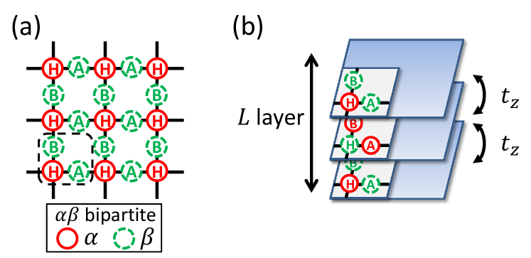
We start by explaining the structure of the multilayer Lieb lattices. Figure 1 (a) depicts the two-dimensional Lieb lattice, where the sites at hubs and spokes are labeled and or , respectively. The dotted square in Fig. 1 (a) represents the unit cell. Figure 1 (b) schematically describes the multilayer lattice with the number of layers of , where the sites in the unit cell are only shown. As illustrated in these figures, the multilayer Lieb lattices are bipartite, where all sites can be classified into sublattice or that have inter-sublattice (-) connections only while no intra-sublattice (- or -) connections. These sublattices are represented as (red) solid and (green) dashed circles in Fig. 1. In general, the magnetism in such bipartite structural lattices can be discussed on the basis of the Lieb theorem.
The Lieb theorem states that, in bipartite lattices, two-component fermions show a finite magnetization with an infinitesimal repulsive interaction at half filling and at zero temperature Lieb (1989). The magnitude of the total magnetization is given by , where () is the total number of the sites in sublattice . Figure 1 clearly shows that, for the multilayer Lieb lattice, sublattice () includes sites ( and ) in the odd-number-th layers and sites and () in the even-number-th layers. The Lieb theorem predicts that the values of per unit cell are for odd and for even in the multilayer Lieb lattices. Note that this theorem does not provide any concrete information about local quantities, such as local magnetization, which can be calculated with the aid of numerical methods.
Our present study is primary concerned about how the interlayer correlations induce the interesting phenomena beyond the predictions of the Lieb theorem. We next show that layered Lieb optical lattices can be derived straightforwardly from the ingenious configuration of lattice lasers. As discussed in Refs. Shen et al. (2010); Apaja et al. (2010), the single-layer (two-dimensional) Lieb lattice can be created by the potential , where is the lattice distance and is the lattice potential depths. The implementation of this complex potential requires several lasers with different wavelengths, e.g., , and Shen et al. (2010); Apaja et al. (2010). On the other hand, we usually apply the additional potential along the direction to confine cold atoms three-dimensionally in the real experiments. As a result, a total potential is
| (1) |
where and are the distance and depth, respectively, for the lattice potential along the direction.
The model Hamiltonian of cold atoms in the potential in Eq. (1) is naturally given by Hubbard Hamiltonian on the layered Lieb lattice, , when and are much larger than the recoil energy of atoms Bloch et al. (2008):
| (2) | |||||
| (3) | |||||
| (4) | |||||
| (5) |
where is an annihilation (creation) operator of an atom with spin at site on the -th layer, and the number operator is defined as . The subscript denotes the summation over the nearest neighbor sites in the plane ( direction). The potentials in Eq. (1), and , determine the intralayer and interlayer hopping amplitude, and , respectively. We assume the present Hamiltonian to be uniform and neglect inhomogeneity due to the trapping potential, which will not change our results qualitatively and just modify them quantitatively. In this paper, we only consider the system at half filling without an external field and at zero temperature as a first step. We set as a unit of energy.
To clearly discuss the interlayer correlation effects on the flat-band magnetism, we investigate the -layer Lieb lattices as shown in Fig. 1 (b) by systematically changing the number of layers as . Here, we set the periodic boundary conditions along the and directions, while an open boundary condition for the direction, which is a natural extension of our previous study for Noda et al. (2009). We also investigate the system with , which corresponds to a three-dimensional layered Lieb lattice with periodic conditions for all three directions. Then, we discuss the asymptotic behaviour from finite to infinite layers, which will show dimensional crossover from the two () to three dimensions () through quasi-three dimensions ().
The two-dimensional Lieb lattice can also be realized in the limit of . Note that this limit is more realistic in experiments, which can be achieved by setting . However, we can at most create an ensemble of the two-dimensional Lieb lattices, and the magnitude of , which is proportional to the laser intensity, is limited for some practical reasons, such as a limitation on the laser power. Therefore, to study the effects of the interlayer correlations on such an ensemble, we investigate the present model Hamiltonian by changing toward a small value. Then, we discuss another dimensional crossover from the (quasi-)three dimensions () to the two dimensions ().
The finite--layer systems can be implemented using the standard experimental techniques. One of the methods is the selection of the layers. For instance, the atoms except for those in the selected layers will be taken away from the lattice with the radio-frequency knife. Another method without the loss of atoms is as follows. We can create an ensemble of the finite--layer lattices by superimposing extra lattice potentials with commensurate wavelengths along the direction. For example, the potential can provide the two-layer [three-layer] Lieb lattice. These simple methods allow us to systematically study the interlayer correlation effects as will be discussed in Sec. IV.
III Method
We use the dynamical mean field theory (DMFT) Metzner and Vollhardt (1989); Georges et al. (1996) to investigate the magnetic properties of multilayer Lieb lattices. In the DMFT framework, each site in the original lattice problem is mapped onto an impurity with hybridization from a dynamical heat bath that effectively describes a connection to surrounding sites. By solving this effective impurity problem in a self-consistent manner, we can precisely deal with local correlation effects, which are essentials for various quantum many-body phenomena, such as the Mott transitions, magnetism, and superconductivity. In fact, the DMFT used for layered systems Potthoff and Nolting (1999); Okamoto and Millis (2004) has successfully demonstrated various phenomena experimentally observed in layered matter, such as a metal-insulator transition at the interface of a heterostructure of transition metal oxides Ohtomo et al. (2002). We comment about our application of DMFT to the Lieb lattice, which consists of different coordination number sites. With the infinitesimal interaction, our DMFT calculations for magnetization, detailed in the next section, are consistent with analytical results described in Appendix. This indicates that our DMFT treatment is efficient to describe the flat-band ferromagnetism, which is one of the main topics of our paper.
To obtain actual DMFT solutions, the effective impurity problem should be solved with the aid of some numerical methods. The solver used in this study is the numerical renormalization group (NRG) Wilson (1975); Bulla et al. (2008). This non-perturbative method can provide numerically exact solutions of the impurity problem in terms of thermodynamic properties at low temperatures. In addition, it can very accurately calculate the low-energy spectral properties at around the Fermi energy. The spectral anomaly of the flat band just at the Fermi energy is the origin of the instability toward magnetic ordering. Thus, the NRG solver can capture the essence of the flat-band magnetism Noda et al. (2009).
Before detailing our DMFT approach, we should mention the unit cells of the present lattices. A unit cell for the two-dimensional Lieb lattice comprises the three sites shown in Fig. 1 (a), and those for the -layer lattices consist of sites. For , the unit cell reduces to sites because of the two-site-period translational symmetry along the direction resulting from the antiferromagnetic ordering along this direction. Note that the ordering pattern we take into account in this study is easily determined from the fact that the layered Lieb lattice is bipartite. The size of the unit cells determines the matrix dimensions of the Green’s function mentioned below.
We explain our DMFT calculations. Here, we self-consistently calculate the local Green’s function of atoms with spin ) at the site ) on the -th layer ():
| (6) |
where is a wave vector , and is the following matrix with a dimension of :
| (7) |
where and are the matrix representation of the Hamiltonians and the Fourier transform of , respectively, and is the identity matrix. The self-energy matrix is diagonal within the DMFT framework, and it is now defined as
where is the self-energy of an atom with spin at site on the -th layer, which can be obtained as mentioned below. Furthermore we set these self-energies to be zero at the first step of iterations. On the other hand, from the Dyson equation, we obtain a cavity Green’s function Georges et al. (1996):
| (8) |
which characterizes the dynamical heat bath connected to an effective impurity that corresponds to an atom with spin at site on the -th layer in the original lattice. By solving such effective impurity problems with the NRG, we obtain self-energy , which allows us to again calculate local Green’s function in Eqs. (6) and (7). This again yields a new , which leads to a new . We perform these calculations repeatedly until convergence. Note that each layer is described by the corresponding three effective impurity problems. Our DMFT formulation for multilayers, which have several sites in the unit cell, is an straightforward extension of the Hubbard model with the antiferromagnetic order in bipartite lattices Georges et al. (1996); Noda et al. (2009).
For , we can straightforwardly extend the above treatment by replacing wave vector in Eqs. (6) and (7) with and replacing in Eq. (7) with the Fourier transform . Here all matrices have a dimension of .
The self-consistently obtained and NRG solutions provide us with various dynamical and thermodynamical quantities. We calculate the magnetization , which are the order parameter of the magnetic transition. In experiments, we can obtain these magnetizations from site- and spin-resolved observations of the number density, e.g., which can be achieved by microscopy and/or spectroscopy. We also calculate the local DOS of the atoms, , which describes the single particle excitation spectra. The local DOS clearly explains various phenomena. For instance, the opening of a spectral gap clarifies the appearance of a metal-insulator transition. This excitation spectra were successfully measured in cold Fermi gases (without lattice potential) by JILA group Stewart et al. (2008). We can expect that this technique will be applicable to lattice systems. When we obtain the complete -resolved excitation spectrum in a lattice, we can construct local DOS that we will discuss in the next section. Furthermore, we note here that the above quantities and satisfy the symmetric relations with respect to and , reflecting a particle-hole symmetry on the AB bipartite lattice under the condition that filling is exactly half in the absence of an external field. These relations are broken when the system is away from at half filling or subject to any external fields, which is beyond the scope of our present study.
IV results
IV.1 Noninteracting DOS

Before discussing magnetism based on the DMFT calculations, to see our way clearly, we first provide the flat-band structures of noninteracting atoms in the multilayer Lieb lattice. Figure 2 shows the DOS for noninteracting atoms at the site on the -th layer () in the -layer lattice for and . Note that the noninteracting DOS is independent of spin , and the mirror symmetries through and planes impose the relations and , respectively. Here, we set .
Figure 2 (a) shows for the two-dimensional Lieb lattice (). We find that the flat-band structure, namely, a delta function resulting from the dispersionless band structure, appears at Fermi energy in the DOS for site , while no flat band appears for site . The flat band at the Fermi energy induces strong instability toward the magnetic ordering, and thus the ferromagnetism appears with the infinitesimal interaction , which can be understood from the well-known Stoner criterion. Note that this mechanism of the flat-band ferromagnetism is consistent with the statement in the Lieb theorem as mentioned in Sec. II.
For multilayer lattices, interlayer hopping affects the flat-band structure in the DOS for site , while it never moves the flat bands to the DOS for the site . As shown in Fig. 2 (b), for , two flat bands appear away from the Fermi energy. Their spectral positions are located at , the estimations of which are detailed in Appendix. For larger , such spectral features depend on layer number . Figure 2 (c) shows that the first layer () in the three-layer lattice has three flat bands at 0 and , while the second layer () has two flat bands at . This difference in the flat-band structure is a key to the magnetism in multilayer lattices, as will be discussed in Secs. IV.2 and IV.3.
Generally, the DOS for the odd-number-th layers in odd--layer lattices have the flat band at , while those for the even-number-th layers in odd--layer lattices and all of the layers in the even--layer lattices do not have the flat band at . Appendix explains this general important feature of the noninteracting DOS in details, and section IV.4 presents the DMFT calculations for general odd- and even--layer lattices.
For , the spectral positions of the (infinite) flat bands become continuous, meaning that the flat-band structure becomes dispersive with the broadening of . However, we find that the instability toward flat-band magnetism still remains in this limit. This striking feature is discussed in Sec. IV.4.
A change in moves the spectral positions of flat bands as mentioned above. We should note that some energy scales related to the flat-band positions are important for understanding the quantitative properties of the magnetic phase transition or crossover in the present system. This point is mainly discussed in Secs. IV.4 and IV.5.
IV.2 Three-layer system as a typical example of odd
Next, we discuss the magnetism in the odd--layer lattices on the basis of the DMFT calculations explained in Sec. III. The noninteracting DOS of these lattices have the flat band at as discussed in Sec. IV.1. In particular, we first pick up the three-layer lattice as an typical example. We set .
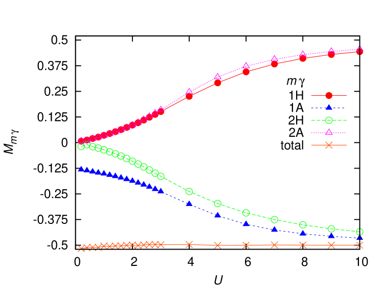
Figure 3 shows sublattice (local) magnetization , where and because of the mirror symmetries. For the magnetization on site , we find characteristic behaviour as follows: Magnetization suddenly becomes a finite value of with the infinitesimal interaction (), and then its magnitude continuously increases with increasing , whereas starts from zero and gradually grows as increases. The singular behaviour, namely, a jump in at , signals the emergence of the ferromagnetic state. In contrast, the second layer () shows no characteristic behaviour: gradually changes in the same manner as .
The -dependent magnetization processes result from the difference in the flat-band structures of the noninteracting DOS as mentioned in Sec. IV.1. Because of the instability resulting from the flat band at the Fermi energy, ferromagnetic ordering immediately occurs with the infinitesimal interaction in the first layer, which leads to a jump in at . On the other hand, all sites in the second layer and also site in the first layer have no flat bands as shown in Fig. 2 (c). The magnetization on these sites is caused by the antiferromagnetic correlation between adjacent sites. Thus, the magnitude of () gradually increases with a sign opposite to (). The magnetic ordering for caused by the instability of the flat band triggers inter- and intra-layer antiferromagnetic correlations.
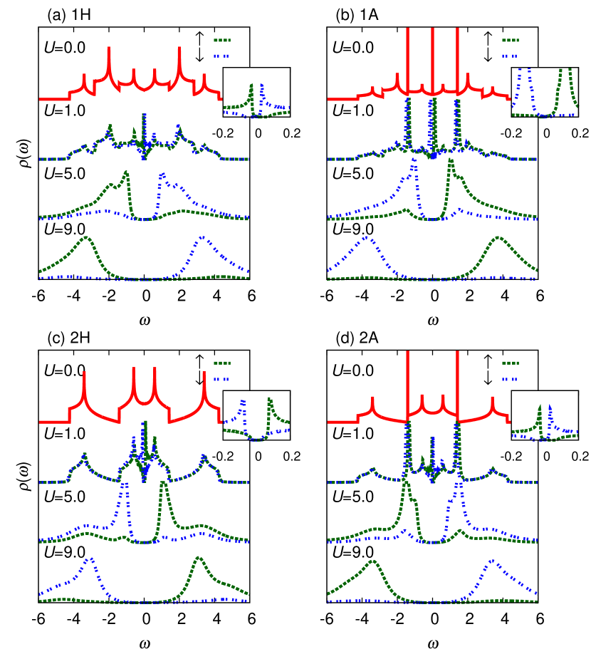
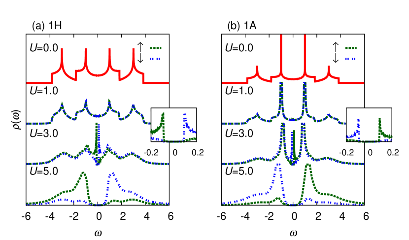
To further discuss the above magnetization process through the dynamical quantities, we calculate the local DOS by changing interaction from weak to strong. We show the results for , , and in Fig. 4, and we also show the noninteracting DOS for comparison, where and because of the mirror symmetries.
We first focus on the DOS for the weak interaction , which are shown in the second spectra from the top in Fig. 4 (a)-(d). By comparing these DOSs with those for , we find that for shows split flat bands at around the Fermi energy, which is clear evidence of the emergence of the ferromagnetic ordering. Importantly, the flat bands away from the Fermi energy are hardly split at all, suggesting that only one flat band just at the Fermi energy can be regarded as the origin of the flat-band instability toward magnetism. We find that the other DOS for also show the gapped structures at the Fermi energy. However, note that these gap structures caused by another mechanism different from the flat-band instability. In fact, as shown in the insets, all gapped structures of the DOS except for show van Hove singularities at the edges of the gaps. The appearance of such band structures after the magnetic transition results from the change of the band structure (band folding) due to the symmetry breaking caused by the antiferromagnetic ordering. Note that for we do not observe this singularity at gap edges Noda et al. (2009) because of the Dirac-semi-metallic feature of the that has no DOS at the Fermi energy [see Fig. 2 (a)].
In the insets of Fig. 4, we find another interesting feature: The gap energies of the DOSs for the sites labeled and are larger than those for and . The former (latter) sites are dominantly occupied atoms (cf. Fig. 3), and the total number of -spin atoms are large as a result of the ferromagnetic ordering. These facts imply that the majority atoms with require a larger energy for the single particle excitation than the minorities. This feature can be seen only in the weakly interacting region as mentioned below.
As increases, for and , the DOS for all sites loses the detailed structures and finally exhibit similar structures that recall upper and lower Hubbard bands. The change in the band structures indicates that the mechanism of the magnetic ordering changes from the flat-band picture to the localized Heisenberg picture, as discussed in the previous study Noda et al. (2009). The occurrence of this crossover can be confirmed from the magnetizations in Fig. 3, where for the strongly interacting region () shows saturation behaviour. We note that, in contrast to the weakly interacting region, the DOS for the strongly interacting one shows no gap-energy difference depending on the site.
We should comment that the magnetism in the general-odd- layers can be understood from the simple extension of the above discussions. This is because, qualitatively, the keys to the magnetism are the flat-band structures as mentioned in Sec. IV.1. The quantitative difference will be discussed below in Sec. IV.4, which also addresses the important question how the magnetism is on the infinite-layer lattice ().
IV.3 Two-layer system as a typical example of even
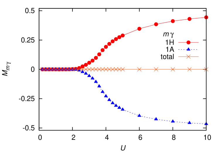
Next, we discuss the magnetism on the even--layer lattices, where the noninteracting DOS have no flat bands at the Fermi energy. We investigate the two-layer lattice with as a typical example of them. The following discussion can be easily extended to general even--layer lattices in the same manner as the odd- case.
Figure 5 shows sublattice magnetizations for , where and because of the mirror symmetries. The magnetization stays zero for the weakly interacting region, and it becomes finite at critical interaction , where a magnetic transition occurs. The suppression of the magnetic ordering for is a consequence of the following facts: Since the DOS for all have no flat bands at the Fermi energy as discussed in Sec. IV.1, there is no flat band instability toward magnetic ordering for small . In addition, we should note that, other kinds of instabilities, such as the nesting, also do not exist. We find that the phase transition occurs when becomes comparable to a specific energy scale , i.e., the difference in the spectral positions of the flat bands for [see Fig. 2 (b) or Appendix]. This can be intuitively understood as follows; an (inelastic) excitation caused by restores the instability of the two flat bands at under the condition .
The above points can be confirmed by the DOS shown in Fig. 6, where symmetries impose and , where is the opposite spin of .
For weak interaction , we find no spectral gap, suggesting no magnetic ordering, while for , we find a gap accompanied with van Hove singularities, which suggests the magnetic ordering with band folding. We can thus conclude that at this is a phase transition from a paramagnetic metal to an antiferromagnetic insulator. Interestingly, the gap structure caused by the restored flat-band instability is analogous to those in the DOS for the sites having no flat bands for (see Fig. 4).
As further increases, the DOS becomes the upper and lower Hubbard bands, suggesting that the localized Heisenberg picture governs the magnetism. By comparing this result with that shown in Fig. 4, we find that the difference in the magnetism between even- and odd--lattices disappears in the Heisenberg limit. This is because the band structure in the space is irrelevant to the magnetism in this limit, whereas the bipartite structure in the space is important. The bipartite structure is the same for all , while the flat-band structure at around the Fermi energy strongly depends on . Note that, even though the odd-even difference in the DOS disappears, the difference in the total magnetization ensured by the Lieb theorem, for odd and 0 for even , is still satisfied due to the alternating ordering along the direction.
IV.4 dependence and the limit
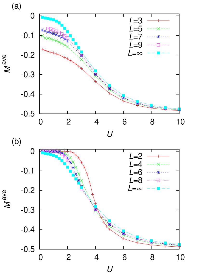
We further investigate the dependences of magnetism, and we also address the infinite-layer lattice that corresponds to the three-dimensional layered Lieb lattice. In Fig. 7, we show the -dependence of the - curves, where is the average magnetization defined as
| (9) |
Here, we add an overall minus sign in Eq. (9) to use the same sign of magnetization of sites where the flat-band ferromagnetic behaviour appears in (see site 1A in Fig. 3). Figure 7 (a) shows that, for odd , average magnetizations in the weak coupling region decrease as increases. On the other hand, Fig. 7 (b) shows that, for even , the critical interaction decreases as increases. In the strongly interacting region, the - curves show the similar behaviour irrespective of whether is even or odd. We confirm the disappearance of the odd-even difference again, which we have already discussed in terms of the DOSs at the Heisenberg limit in the last paragraph in Sec. IV.C. We also find that the curves for both odd- and even--layer lattices naturally approach those in the same limit of (the three-dimension limit).
As shown in Fig. 7, in the three-dimensional layered Lieb lattice (), we find that the magnetic ordering appears at infinitesimal . The asymptotic behaviour of odd--layer lattices indicates that this magnetism for is a consequence of the flat-band instability. On the other hand, in the even- layer lattices without flat-band instability, the curious asymptotic behaviour (i.e., the decrease in with increasing ) reflects the striking feature: the flat-band instability is restored with infinitesimal at with . This completely contradicts our naive expectation that the three-dimensional lattice () will show a finite critical , because the flat band becomes dispersive with a broadening of as mentioned in Sec. IV.1 (and also in Appendix).
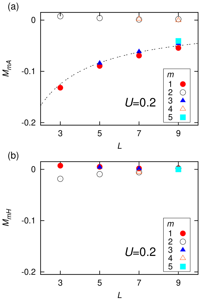
We discuss the asymptotic behaviour with increasing in more detail. We first show the results for the odd--layer lattices and focus on a characteristic quantity , the magnetization at infinitesimal . Figure 8 shows calculated by changing the natural number with , where we set to a rather large value of because of the numerical limitation. We find for odd is proportional to , while for even and for all stay zero (within the present numerical precision). This difference between even and odd is attributed to the noninteracting DOS. We can simply explain the origin of behaviour for odd as follows: The -layer lattices have multibands, and only one of the bands, that is, the flat band at the Fermi energy, takes part in the ferromagnetism with infinitesimal . This means that the weight of the flat-band related to the ferromagnetism decreases with increasing as . The dotted line shows the asymptotic behaviour , which is evaluated analytically beyond the above intuitive discussions (see Appendix). The Lieb theorem provides the same conclusion: the difference in the number of sublattices stays one as increases even though the unit cell size increases as .
We also explain the asymptotic behaviour in the even--layer lattices. The characteristic of even lattices is the finite critical interaction . As mentioned in Sec. IV.3, the magnetism occurs when the strength of interaction becomes comparable to the energy difference in the spectral positions of the two flat bands nearest to the Fermi energy, where the flat-band instability is restored as discussed in Sec. IV.3. As derived in Appendix, we find , which determines the asymptotic behaviour of the even--layer lattices shown in Fig. 7 (b). This clearly shows that the flat-band instability is restored with infinitesimal at , and the difference between even and odd naturally disappears at .
IV.5 dependence and the limit
We finally investigate the dependence of the magnetism by changing toward . In the limit of , the present system for all becomes equivalent to the two-dimensional lattice that has already been investigated in Ref. Noda et al. (2009). We thus perform the calculations on the three-layer lattice for small and compare these results with those for already shown in Fig. 3.
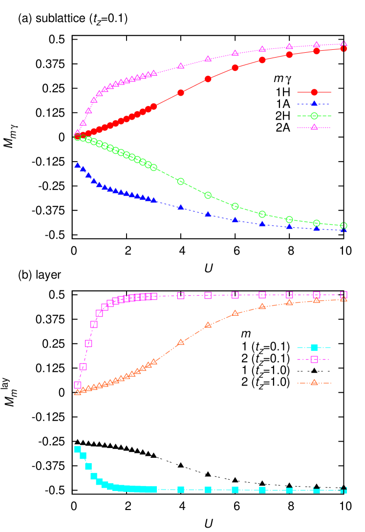
Figure 9 (a) shows the sublattice magnetization for as a function of . We find that for steeply grows for , and then it gradually grows for and shows saturation at around . On the other hand, for shows no characteristic behaviour at around and shows saturation similar to the above at around . The difference between for and sites is attributed to the flat bands that appear only in . The saturations for both and suggest the crossover from the flat band to the Heisenberg magnetisms as already mentioned above. For small , at around , we observe the characteristic behaviour not observed in for (see Fig. 3).
To clarify the difference between the results for smaller and larger , we also show in Fig. 9 (b) the layer magnetization defined as , which characterizes the (macroscopic) population imbalance between the and atoms in the corresponding layer . Note that, with the infinitesimal interaction, this layer magnetization also shows a clear jump, which is a feature of the flat-band ferromagnetic state. We find that shows saturation behaviour at around . This suggests that the layer magnetization clearly signals the crossover. The saturated layer magnetization shows antiferromagnetic alternating behaviour: . Note that, in the two-dimensional Lieb lattice (), the layer magnetization always stays at 0.5 when is finite, which is a manifestation of the Lieb theorem. From this point, we can understand the origin of the crossover at around as follows: for , only one of the flat bands at the Fermi energy takes part in the flat-band magnetism as discussed above (see Fig. 4 and related discussions in Sec. IV.2). In contrast, for , all of the flat bands join the magnetic ordering, even though they are not at the Fermi energy. The latter situation can be regarded as analogous to the flat-band magnetism seen in the ensemble of two-dimensional Lieb lattices. We should note that the interlayer hopping still causes antiferromagnetic correlations between the Lieb lattices.
We can thus conclude that the crossover at for originates from the change in the picture of the magnetism from that in the quasi-three-dimensional layered Lieb lattice to that in the correlated ensemble of the two-dimensional Lieb lattice. We can now evaluate that the crossover occurs when becomes much larger than , which corresponds to the energy difference between the two flat bands farthest from the Fermi energy (see Appendix). For (and also larger ), this crossover cannot be seen, because it is covered by the flat-band to Heisenberg crossover that occurs when becomes comparable to the bandwidth of the two-dimensional Lieb lattice . In the Heisenberg limit, the flat-band structure is irrelevant to the magnetism, which can be confirmed from the fact that the DOS for strong shows no band structures except for the upper and lower Hubbard bands as mentioned above and also in Ref. Noda et al. (2009).
V conclusions
We investigate the magnetic properties of two-component fermions in a multilayer Lieb lattice at half filling and at zero temperature using the DMFT combined with the NRG. We elucidate that even- and odd- layers show different magnetization behaviours. The flat-band ferromagnetic state appears only in odd- layers. For even- layers, the transition occurs when the interaction restores the flat-band instability toward the antiferromagnetic ordering. This odd-even difference disappears in the limit of . On the other hand, as common features seen in all layers, the magnetic properties in the weak interaction region are dominated by flat bands, while those in the strong interaction region can be well understood by the Heisenberg spin picture. We further elucidate the interlayer correlation effects, which induce another crossover and the antiferromagnetic correlations between layers.
In this paper, we restrict our calculations to zero temperature. It is also important to briefly discuss the property at finite temperatures. We expect that we can observe finite transition temperatures in the present multilayer Lieb lattices thanks to the weak three-dimensional effects, although the Marmin-Wagner theorem theoretically prohibits the transition in such quasi-two dimensional systems. From the numerical results, we have revealed the crossover from the flat-band to the Heisenberg picture with increase in the interaction strength. This clearly indicates that the transition temperature is the highest in the crossover region by noting the same mechanism appearing in the cubic lattice Pruschke2005 . An interesting future work is to extend our theory to the case at finite temperatures. We will address this problem and publish it elsewhere.
We mention experimental advantages of making the multilayer structure. First, we can detect the flat-band ferromagnetic state by only measuring layer magnetizations without addressing sublattice magnetization as shown in Fig. 9 (b). This is a novel property of the multilayer Lieb lattice. Second, magnetic correlations in a multilayer system can be enhanced by the following experimental technique. In Ref. Greif et al. (2013), the ETH group adiabatically changed the cubic lattice to an anisotropic or dimerized cubic lattice. This process causes local redistribution of entropy, leading to a great enhancement of the short-range magnetic correlation. They successfully observed the enhanced magnetic correlation. For multilayer Lieb lattices, we can also adiabatically induce anisotropic interlayer hopping by applying additional lasers in the direction. The entropy redistribution similarly enhances the magnetic correlation inside the multilayer system. These two advantages encourage us to consider the multilayer lattices as promising candidates for observing the flat-band ferromagnetic state.
VI acknowledgements
We are grateful to N. Kawakami and Y. Takahashi for valuable discussions. This work was partly supported by Grants-in-Aid for Scientific Research (No. 25287104).
*
Appendix A
This appendix shows simple analytical discussions about the local DOS of the noninteracting atoms in the -layer Lieb lattices with an open boundary condition along the direction. We calculate the spectral positions and weights of flat bands in the noninteracting local DOS, and we simply explain why the difference between odd and even appears. We also address what determines the asymptotic behaviour from the finite--layer to the three-dimensional (infinite) layer Lieb lattices for both even and odd .
Here, we discuss the noninteracting local DOS for with and . The DOS for is of the well-known two-dimensional Lieb lattice [see Fig. 2 (a)]. It is convenient to use the following expression for them: . The DOS for multilayer lattices with can be obtained by the simple extension from the two-dimensional case because the noninteracting Hamiltonian, , can be solved by variable separation. Namely, is written as follows:
| (10) |
where and are eigenvalues and corresponding eigenvectors of the following matrix with a dimension of :
| (11) |
This matrix is the submatrix of defined in the main text. Figure 2 confirms the above discussion. This matrix can be solved analytically, which is shown in detail with our physical interpretation in the following several paragraphs. Those who are familiar with this solution can skip those paragraphs.
In what follows, for simplicity, we only focus on the flat bands and neglect the other DOS structures. This simplification is very rough but well describes the physics of the flat-band magnetism that occurs at the infinitesimal . This simplification yields and . The positions (weights) of the flat bands in are determined from (). Note that the sum rule should be satisfied because we now consider only flat bands and neglect the other bands.
The eigenvalues in energy units of can be calculated from the following recurrence relation:
| (12) |
where is equivalent to and the eigenvalues satisfy . On the other hand, the eigenvectors can be calculated from , which can be rewritten as
| (13) |
where and . The obtained eigenvectors should be normalized as .
Equation (12) clearly explains why the difference between even and odd layers appears. With , Eq. (12) reduces to with and . This means that the flat band at the Fermi energy appears only for odd .
From Eq. (13), we can discuss the asymptotic behaviour of , the magnetization at infinitesimal interaction , for odd with a natural number. Substituting into Eq. (13), we obtain the corresponding renormalized eigenvector as , which means that the weights of the flat band at the Fermi energy in local DOS are for odd-number-th layer and 0 for even-number-th layer. This clearly shows that the flat-band magnetism appears only in the odd-number-th layers. The weights of the flat bands determine that for odd asymptotically decreases with , where the factor of results from in the definition of and in shown above while that for even stays . These are numerically confirmed as shown in Fig. 8 and discussed in Sec. IV.4.
Furthermore, we can discuss the critical interaction strength for even . As discussed in Sec. IV.3, we assume that the critical can be determined from the energy difference between the two flatbands nearest the Fermi energy. From Eq. (12), we can derive the explicit representation of the eigenvalues as . We obtain for large . This means that the critical interaction strength also shows ()-asymptotic behaviour as discussed in Sec. IV.4. We should comment that neglecting the DOS except for the flat band as mentioned above is actually an oversimplification due to the finite (not infinitesimal) critical interaction. Nevertheless, our numerical results with show a good agreement with the above simple analysis. For example, as shown in Fig. 5, the critical for is about .
We mention another energy scale , which represents the energy difference between the two flat bands farthest from the Fermi energy. We can rewrite , which reduces to for a large . Note that can be regarded as the bandwidth of broadened flat bands in the limit of , and the total bandwidth of the three bands in this three-dimensional limit is given by . This energy scale determines the characteristic crossover discussed in Sec. IV.5.
References
- Bloch et al. (2008) I. Bloch, J. Dalibard, and W. Zwerger, Rev. Mod. Phys. 80, 885 (2008).
- Esslinger (2010) T. Esslinger, Annu. Rev. Condens. Matter Phys. 1, 129 (2010).
- Jordens et al. (2008) R. Jordens, N. Strohmaier, K. Gunter, H. Moritz, and T. Esslinger, Nature 455, 204 (2008).
- Schneider et al. (2008) U. Schneider, L. Hackermller, S. Will, T. Best, I. Bloch, T. A. Costi, R. W. Helmes, D. Rasch, and A. Rosch, Science 322, 1520 (2008).
- Becker et al. (2010) C. Becker, P. Soltan-Panahi, J. Kronjäger, S. Dörscher, K. Bongs, and K. Sengstock, New J. Phys. 12, 065025 (2010).
- Wirth et al. (2011) G. Wirth, M. Olschlager, and A. Hemmerich, Nat. Phys. 7, 147 (2011).
- Soltan-Panahi et al. (2011) P. Soltan-Panahi, J. Struck, P. Hauke, A. Bick, W. Plenkers, G. Meineke, C. Becker, P. Windpassinger, M. Lewenstein, and K. Sengstock, Nat. Phys. 7, 434 (2011).
- Jo et al. (2012) G.-B. Jo, J. Guzman, C. K. Thomas, P. Hosur, A. Vishwanath, and D. M. Stamper-Kurn, Phys. Rev. Lett. 108, 045305 (2012).
- Tarruell et al. (2012) L. Tarruell, D. Greif, T. Uehlinger, G. Jotzu, and T. Esslinger, Nature 483, 302 (2012).
- Uehlinger et al. (2013) T. Uehlinger, G. Jotzu, M. Messer, D. Greif, W. Hofstetter, U. Bissbort, and T. Esslinger, Phys. Rev. Lett. 111, 185307 (2013).
- Lieb (1989) E. H. Lieb, Phys. Rev. Lett. 62, 1201 (1989).
- Mielke (1991) A. Mielke, J. Phys. A: Math. Gen. 24, 3311 (1991).
- Tasaki (1992) H. Tasaki, Phys. Rev. Lett. 69, 1608 (1992).
- Mielke and Tasaki (1993) A. Mielke and H. Tasaki, Comm. Math. Phys. 158, 341 (1993).
- Tasaki (2008) H. Tasaki, Eur. Phys. J. B 64, 365 (2008).
- Shen et al. (2010) R. Shen, L. B. Shao, B. Wang, and D. Y. Xing, Phys. Rev. B 81, 041410 (2010).
- Apaja et al. (2010) V. Apaja, M. Hyrkäs, and M. Manninen, Phys. Rev. A 82, 041402 (2010).
- (18) Y. Takahashi, International Conference on Atomic Physics (ICAP) 2014 abstract .
- Noda et al. (2009) K. Noda, A. Koga, N. Kawakami, and T. Pruschke, Phys. Rev. A 80, 063622 (2009).
- Weeks and Franz (2010) C. Weeks and M. Franz, Phys. Rev. B 82, 085310 (2010).
- Goldman et al. (2011) N. Goldman, D. F. Urban, and D. Bercioux, Phys. Rev. A 83, 063601 (2011).
- Zhao and Shen (2012) A. Zhao and S.-Q. Shen, Phys. Rev. B 85, 085209 (2012).
- Niţă et al. (2013) M. Niţă, B. Ostahie, and A. Aldea, Phys. Rev. B 87, 125428 (2013).
- Ohtomo et al. (2002) A. Ohtomo, D. A. Muller, J. L. Grazul, and H. Y. Hwang, Nature 419, 378 (2002).
- Castro Neto et al. (2009) A. H. Castro Neto, F. Guinea, N. M. R. Peres, K. S. Novoselov, and A. K. Geim, Rev. Mod. Phys. 81, 109 (2009).
- Hwang et al. (2012) H. Y. Hwang, Y. Iwasa, M. Kawasaki, B. Keimer, N. Nagaosa, and Y. Tokura, Nat. Mater. 11, 103 (2012).
- Metzner and Vollhardt (1989) W. Metzner and D. Vollhardt, Phys. Rev. Lett. 62, 324 (1989).
- Georges et al. (1996) A. Georges, G. Kotliar, W. Krauth, and M. J. Rozenberg, Rev. Mod. Phys. 68, 13 (1996).
- Potthoff and Nolting (1999) M. Potthoff and W. Nolting, Phys. Rev. B 59, 2549 (1999).
- Okamoto and Millis (2004) S. Okamoto and A. J. Millis, Phys. Rev. B 70, 241104 (2004).
- Wilson (1975) K. G. Wilson, Rev. Mod. Phys. 47, 773 (1975).
- Bulla et al. (2008) R. Bulla, T. A. Costi, and T. Pruschke, Rev. Mod. Phys. 80, 395 (2008).
- Stewart et al. (2008) J. T. Stewart, J. P. Gaebler, and D. S. Jin, Nature 454, 744 (2008).
- (34) Th. Pruschke, Prog. Theor. Phys. 160, 274 (2005).
- Greif et al. (2013) D. Greif, T. Uehlinger, G. Jotzu, L. Tarruell, and T. Esslinger, Science 340, 1307 (2013).