One, Two, Zero : Scales of strong interactions

Abstract

We discuss our results on QCD with a number of fundamental fermions ranging from zero to sixteen. These theories exhibit a wide array of fascinating phenomena which have been under close scrutiny, especially in recent years, first and foremost is the approach to conformality. To keep this review focused, we have chosen scale generation, or lack thereof as a guiding theme, however the discussion will be set in the general framework of the analysis of the phases and phase transitions of strong interactions at zero and nonzero temperature.

I Adding matter : QCD with an arbitrary flavor number

Usual QCD dynamics is characterized by spontaneous symmetry breaking and dynamical mass generation, with the associated scale $\Lambda_{\mathrm{QCD}}$. However, when the number of flavors exceeds a critical number, an infra-red fixed point (IRFP) appears and prevents the coupling from growing large enough to break chiral symmetry. The theory is then scale invariant - even conformal invariant. In the intermediate region, the coupling ‘walks’ rather than runs between two typical scales - this is the phenomena of scale separation for which our results provide a preliminary evidence. From a general field theory viewpoint, the analysis of the phase diagram of strong interactions as a function of the number of flavor adds to our knowledge of the theoretical basis of strong interactions and their fundamental mechanisms. From a phenomenological viewpoint, this study deals with a class of models which might play a relevant role in model building beyond the standard model (BSM) SCGT ; Ph_review ; Yamawaki:1985zg ; Holdom:1984sk ; Akiba:1985rr ; Appelquist:1986an , which explain the origin of mass using strong coupling mechanisms realized in QCD with a large number of flavors. All these topics are under active scrutiny both theoretically and experimentally Lat1 ; Lat2 ; Lat3 ; Lat4 ; Itou:2013ofa ; Appelquist:2011dp ; Appelquist:Conformal ; Appelquist:2009ka ; Appelquist:2010xv ; Deuzeman:2008sc ; Deuzeman:2009mh ; Deuzeman:2012ee ; Deuzeman:2012pv ; Miura:2011mc ; Miura:2012zqa ; Aoki:2014oha ; Aoki:2013zsa ; Aoki:2013xza ; Aoki:2012eq ; Cheng:2014jba ; Cheng:2013eu ; Cheng:2011ic ; Hasenfratz:2011xn ; Hasenfratz:2010fi ; Hasenfratz:2009ea ; Fodor:2011tu ; Fodor:2009wk ; Ishikawa:2013tua ; Ishikawa:2013wf ; Iwasaki:2003de ; Finland:MWT ; Svetitsky:sextet ; Kogut:2010cz ; Fodor:2009ar ; Fodor:2012ty ; Catterall:MWT ; Lucini:MWT ; DelDebbio:2010jy ; DelDebbio:2010ze ; deForcrand ; BraunGies ; EKMJ ; Alho:2012mh ; Gursoy:2010fj ; Alho:2013dka ; Liao:2012tw ; Ryttov:2012nt ; Ryttov:2007cx ; Dietrich:2006cm ; Antipin:2012sm ; Matsuzaki:2013eva ; Matsuzaki:2012xx

I.1 Conformality

Conformal invariance is anticipated to emerge in the non-Abelian gauge theory with many species (flavors) of fermions Caswell:1974gg ; Banks:1981nn ; Appelquist ; Miransky:1997 ; Appelquist:1999hr . This is due to the IRFP for $N_{f}>N_{f}^{*}$ at a coupling which is not strong enough to break chiral symmetry: a second zero of the two-loop beta-function of a non-Abelian gauge theory implies, at least perturbatively, the appearance of IRFP conformal symmetry Caswell:1974gg ; Banks:1981nn . In color SU($3$) gauge theory with $N_{f}$ massless fundamental fermions, the second zero appears at $N_{f}\gtrsim 8.05$, before the loss of asymptotic freedom (LAF) at $N_{f}^{\mathrm{LAF}}=16.5$. Analytic studies of the conformal transition of strong interactions have produced a variety of predictions for the conformal threshold: the Schwinger-Dyson approach with rainbow resummations Appelquist ; Miransky:1997 ; Appelquist:1999hr or the functional renormalization group method BraunGies suggest the onset of conformal window around $N_{f}^{*}\sim 12$. An all-order perturbative beta-function Ryttov:2007cx inspired by the Novikov–Shifman–Vainshtein–Zakharov beta-function of SQCD Novikov:1983uc leads to a bound $N_{f}^{*}>8.25$. Instanton studies at large $N_{f}$ Velkovsky:1997fe claimed a qualitative change of behaviour at $N_{f}=6$. The $N_{f}^{*}$ has also been estimated for different fermion representations Dietrich:2006cm . Holographic models for QCD in the Veneziano limit find $3.7<(N_{f}/N_{c})^{*}<4.2$ EKMJ .

I.2 Pre-conformality

The direct inspection of theories at fixed $N_{f}$ is often inconclusive, especially close to the expected threshold $N_{f}^{*}$.

An alternative approach to establish the existence of the conformal window is to (try to) observe directly the approach to conformality by monitoring the evolution of the results obtained in the broken phase as a function of $N_{f}$.

Moreover, the pre-conformal dynamics at flavor numbers just before the onset of conformal invariance might serve as a paradigm for the BSM model buildings that invokes non-perturbative mechanisms of electroweak symmetry breaking Yamawaki:1985zg ; Holdom:1984sk ; Akiba:1985rr ; Appelquist:1986an . In such pre-conformal region, the coupling should vary little – should walk – with the scale, at variance with the familiar running of QCD. One important question, of genuinely theoretical nature, is to establish the existence and uncover the properties of this new class of strongly interacting (quasi) conformal theories. Because of this, the sub–critical region, when $N_{f}$ gets closer and closer to $N_{f}^{*}$, is interesting per se. Ph_review . In our study, such pre-conformal dynamics could manifest itself either with a clear observation of a separation of scales, or with a manifestation of a critical behaviour when approaching $N_{f}^{*}$. One possibility is to observe the Miransky-Yamawaki essential singularity Miransky:1997 . Alternatively, in an FRG approach BraunGies , the pseudo-critical line is almost linear with $N_{f}$ for small $N_{f}$, and displays a singular behaviour when approaching $N_{f}^{*}$, which could be the only observable effects, beyond Miransky scaling. A jumping scenario in which the change from a QCD dynamics to the conformal window is abrupt is also a distinct possibility Antipin:2012sm .

I.3 The high temperature path to conformality

Chiral symmetry is restored at high temperatures – in the so-called quark-gluon plasma (QGP) phase. Both physics intuition and phenomenological analysis based on functional renormalization group BraunGies and finite temperature holographic QCD Alho:2012mh indicate that the conformal phase of cold, many flavor QCD and the high temperature chirally symmetric phase are continuously connected. In particular, the onset of the conformal window coincides with the vanishing of the transition temperature, and the conformal window appears as a zero temperature limit of a possibly strongly interacting QGP.

The analysis of the finite temperature phase transition is a well-established line of research within the lattice community. In our approach we build on this experience and use the properties of a thermal system to learn about general aspects of the phase diagram also at zero temperature. According to the Pisarski-Wilczek scenario Pisarski:1983ms , the most likely possibility for $N_{f}\geq 3$ is a first order chiral transition in the chiral limit, turning into a crossover above a critical mass endpoint, and/or on lattices which are not large enough. However it should be noted that closer to the conformal window the dynamics of the light scalar mode might invalidate this simple picture, and the nature of the thermal transitions poses specific issues. We will identify the thermal crossover with confidence for a number of flavors ranging from four to eight, and we will complement these results with those of the deconfinement transition in the quenched model. Then, we study the approach to the conformal phase in the light of the chiral phase transition at finite temperature with variable number of flavors. Further, we will argue that even results in the bare lattice parameters can be used directly to locate the critical number of flavors, thus generalising to finite temperature the Miransky-Yamawaki phase diagram, Ref. Miransky:1997 .

I.4 Setting the scale

One ubiquitous problem in these studies is the setting of a common scale among theories which are essentially different. We propose two alternative possibilities to handle this problem, one stemming from our own work Miura:2011mc ; Miura:2012zqa , and the other from a recent analysis Liao:2012tw . Interestingly, this latter approach analyses the dependence of the confinement parameters on the matter content, and proposes microscopic mechanisms for confinement motivated by such $N_{f}$ dependence.

I.5 Sketching the phase diagram

The phase diagram of QCD emerging from these discussions is sketched in Fig. 1: the axis is simply the number of light flavors. Ordinary QCD – two light flavors – is marked by an arrow. The conformal region is on the right hand side, and is separated by the essential singularity for a critical number of flavor (of about eleven according to the current estimates) from the hadronic phase. The possibility of a first order transition has been discussed as well, and we will get back to this later in this paper. Clearly, as in any system undergoing a phase transition, the nature and extent of the critical window are purely dynamical questions whose answer cannot be guessed a priori. Since the underlying dynamics is completely non-perturbative, lattice calculations are the only tool to perform an ab initio, rigorous study of these phenomena, and many lattice studies have recently appeared Lat1 ; Lat2 ; Lat3 ; Lat4 .

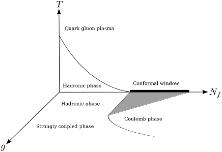
Figure 1: A projected view of the phase diagram of QCD-like theories in the temperature ($T$), flavor number ($N_{f}$) and bare coupling ($g$) space. In the T-$N_{f}$ plane, the critical line is a phase boundary between the chirally broken hadronic phase and the chirally symmetric quark gluon plasma, the zero temperature end point of which is the onset of the conformal window. The zero temperature projected plane is inspired by the scenario in Refs. Appelquist:1999hr ; Miransky:1997 .

We now turn to the presentation of our results. The interested reader can find all the details in our published papers Deuzeman:2008sc ; Deuzeman:2009mh ; Deuzeman:2012ee ; Miura:2011mc ; Miura:2012zqa , and we here omitted many (sometimes important) details for the sake of a more concise presentation. Section II is devoted to the strategies we have used to obtain an (indirect) evidence of conformality from a direct evidence of chiral symmetry restoration. Some comments on the mass anomalous dimension associated with our measurements are included as well.

In Sec. III, we investigate the chiral phase transition at finite temperature for various numbers of flavor, and evaluate the onset of the conformal window $N_{f}^{*}$ via the vanishing of the transition temperature at large $N_{f}$. The results are further exploited in Sec.IV to highlight a connection between the conformal window and a cold QGP. In Sec. V, we discuss the issues of scale separation and possible direct evidence, which are still work in progress. In Sec. VI, we will summerize our review.

II The quest for conformality

In this Section, we discuss the existence of a conformal phase in $SU(N_{c}=3)$ gauge theories in four dimensions. In this lattice study, we explore the model in the bare parameter space, varying the lattice coupling and bare fermion mass.

The analysis of the chiral order parameter and the mass spectrum of the theory indicates the restoration of chiral symmetry at zero temperature and the presence of a Coulomb-like phase, depicting a scenario compatible with the existence of an IRFP at nonzero coupling.

Following the T=0 plane of Fig. 1, at a given $N_{f}>N^{*}_{f}$ and increasing the gauge coupling from $g=0$, one crosses the line of the IRFPs, going from a chirally symmetric and asymptotically free phase (pre-conformal phase, shaded in the picture) to a symmetric, but not asymptotically free one (Coulomb-like or QED-like phase). A phase transition need not be associated with the line of IRFPs, differently from what was originally speculated in Ref. Banks:1981nn . At even larger couplings, a transition to a strongly coupled chirally asymmetric phase will always occur in the lattice regularized theory. The latter is referred to as a bulk phase transition. In the symmetric phases at nonzero coupling the conformal symmetry is still broken by ordinary perturbative contributions. They generate the running of the coupling constant which is different on the two sides of the symmetric phase. See Ref. Miransky:1997 for a detailed discussion of this point. We emphasize that in the region considered in this paper the conformal symmetry would still be broken by Coulombic forces.

One lattice strategy to assess conformality was then the following: first, it was demonstrated that the location of the transition from the chirally symmetric to the broken phase is not sensitive to the physical temperature and is therefore compatible with a bulk nature. Subsequently, the bare fermion mass dependence of the chiral condensate on the weak coupling side of the bulk transition clearly favored a chiral symmetry restoration. Finally, the behavior of the mass spectrum close to the bulk transition will be studied, again confirming chiral symmetry restoration without making use of detailed fits. The mass dependence of the spectrum allowed the extraction of a candidate mass anomalous dimension. These results are consistent with the scenario for conformality of Fig. 1. In the following, we limited ourselves to the presentation of the spectrum results which are probably those providing a cleanest visual evidence, and which have been updated and expanded very recently.

All our simulations use staggered fermions (Kogut-Susskind) in the fundamental representation in color $SU(N_{c}=3)$. Here we used a tree level Symanzik improved gauge action to suppress lattice artifacts, and staggered fermions with the Naik improvement scheme, that effectively extends the Symanzik improvement to the matter content.

II.1 Spectrum

It has been noted in the past that one can devise robust signatures of chiral symmetry based on the analysis of the spectrum results. One first significant spectrum observable is the ratio $m_{\pi}/m_{\rho}$, between the mass of the lightest pseudoscalar state (pion) $m_{\pi}$ and the mass of the lightest vector state (rho) $m_{\rho}$. In real-life QCD at zero temperature, chiral symmetry is spontaneously broken and the pion is the (pseudo)Goldstone boson of the broken symmetry, implying that its mass will behave as $m_{\pi}\sim\sqrt{m}$. In contrast, chiral symmetry is restored in the continuum limit in the conformal window. At the IRFP and at infinite volume, the quark mass dependence of all hadron masses in the spectrum is governed by conformal symmetry: at leading order in the quark mass expansion all masses follow a power-law with common exponent determined by the anomalous dimension of the fermion mass operator at the IRFP. Hence we expect a constant ratio. Away from the IRFP, for sufficiently light quarks and finite lattice volumes, the universal power-law dependence receives corrections, due to the fact that the theory is interacting but no longer conformal.

The behaviour of the ratio is demonstrated in Fig. 3: a conformal scenario seems favoured in the range of masses we are exploring. Note that the $m_{\pi}/m_{\rho}$ ratio should go to zero in the chiral limit in the broken phase, and to a constant value if chiral symmetry is restored.

Analogous conclusions can be drawn from the inspection of so-called an Edinburgh plot Fig. 3. The difference with the case of ordinary QCD is indeed striking. The modest scattering of the data points could be ascribed to the deviation from a perfect power law as discussed above. It would then be of interest to repeat the same plot for different couplings : at the IRFP it should indeed reduce to a point.

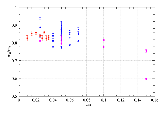
Figure 2: Ratio $m_{\pi}/m_{\rho}$ as a function of the bare quark mass for all existing data for $N_{f}=12$, and $N_{f}=16$: $N_{f}=12$ data from Fodor:2011tu (red squares), our $N_{f}=12$ data and $\beta_{L}=3.8,3.9,4.0$ (blue circles), $N_{f}=16$ data from Damgaard:1997ut (magenta diamonds).

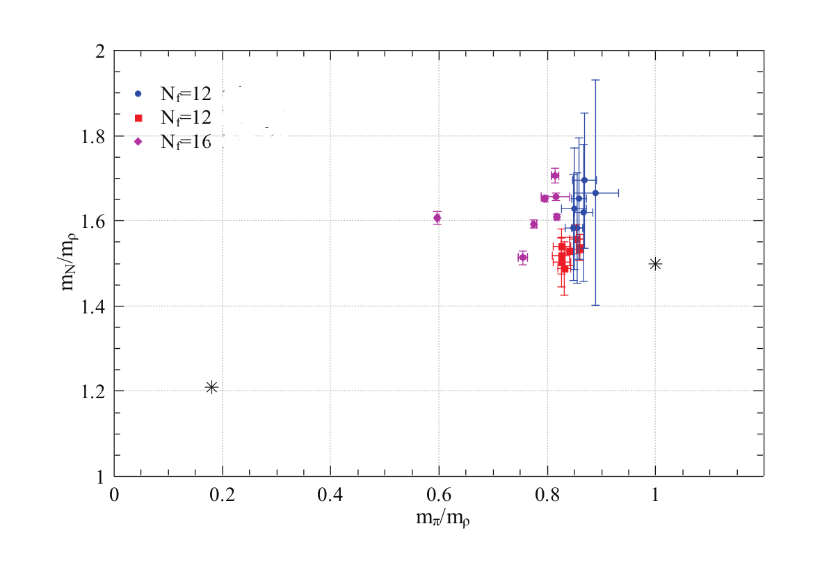
Figure 3: Edinburgh plot: $N_{f}=12$ data from Fodor:2011tu (red squares), our $N_{f}=12$ data and $\beta_{L}=3.8,3.9$ (blue circles), $N_{f}=16$ data from Damgaard:1997ut (magenta diamonds). The QCD physical point (black star, leftmost) and the heavy quark limit (free theory) point (black star, rightmost) are shown.

II.2 Anomalous Dimension

To see whether the theory has the anomalous dimension for $N_{f}=12$, we plot the pseudoscalar mass as a function of the chiral condensateKocic:1992is , as in Fig. 4. The data are best fitted by a simple power-law form $(am_{\pi})^{2}=A(a^{3}\langle\bar{\psi}\psi\rangle)^{2\delta_{\chi}}$, with $\delta_{\chi}=0.64(1)$. They clearly suggest that chiral symmetry is restored and that the theory has anomalous dimensions Kocic:1992is . For comparison, in the symmetric phase and in mean field we expect a linear dependence with non negative intercept. The presence of anomalous dimensions is responsible for negative curvature - noticeably opposite to what finite volume effects would induce - and a zero intercept. The same graph in the broken phase would show the opposite curvature and extrapolate with a negative intercept.

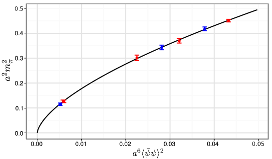
Figure 4: The relation between the chiral condensate and the pion mass, for $6/g_{L}^{2}$ = 3.9 (blue) and 4.0 (red). The line represents a power law fit to the combined data

Further, in Fig. 5 we report on the measured values of $m_{\pi}$ and $m_{\rho}$ as a function of the bare fermion mass from our early work Deuzeman:2009mh . Here the lightest point at $am=0.025$ for the vector mass is absent, but a curvature can still be appreciated. Simulations were done on $16^{3}\times 24$ volumes, while a set of measurements at larger volumes showed that finite volume effects were under control. The mass dependence shown in Fig. 5 hints again at a few properties of a chirally symmetric phase. We have fitted both the pion and the rho mass with a power law ansatz

$$m_{\pi,\rho}=A_{\pi,\rho}m^{\epsilon_{\pi,\rho}}$$ (1)

and obtained the results $A_{\pi}=3.41(21)$, $\epsilon_{\pi}=0.61(2)$, $A_{\rho}=4.47(61)$, $\epsilon_{\rho}=0.66(5)$ at $6/g_{L}^{2}=3.9$, and $A_{\pi}=3.41(21)$, $\epsilon_{\pi}=0.61(2)$, $A_{\rho}=4.29(11)$, $\epsilon_{\rho}=0.66(1)$ at $6/g_{L}^{2}=4.0$. The accuracies of these fits are not comparable with those achieved by the fits to the chiral condensate, however they allow to draw a few conclusions. First, the mass dependence of the vector and pseudoscalar mesons is well fitted by a power-law. Second, it is also relevant that the exponents are not unity and $\epsilon_{\pi}\neq 1/2$. The latter result immediately tells that the pion seen here is not a Goldstone boson of a broken chiral symmetry. In addition, both mesons have masses scaling with roughly the same power, as it should be in a symmetric phase, and with increasing degeneracy towards the chiral limit. The exponent of the power law being not one, confirms that we are not in the heavy quark regime. From the results for the exponent $\epsilon$ we can formally extract a value for the anomalous dimension consistent with the other lattice results as well as the analytic estimates Itou:2013ofa . Needless to say, a full control on the systematic and on the corrections to scaling is needed before making such identification with confidence.

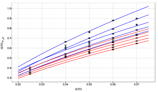
Figure 5: The relation between the bare quark mass and the masses of the pion (red) and rho meson (blue), for $6/g_{L}^{2}$ = 3.6, 3.7, 3.8, 3.9 and 4.0 from the uppermost line down. Power law fits to the separate values of beta are provided.

II.3 Inside the conformal phase : lattice matters at strong coupling!

We have previously discussed a strong coupling zero temperature transition – a bulk transition – within the conformal window. However, if we were to use a perfect action, the conformal phase discussed above would extend all the way till the infinite coupling limit. The role of improvement in this case is really dramatic! A perfect action would destroy a phase transition. No surprise, of course: these are strong coupling phenomena taking place away from the continuum limit, hence extra terms in the actions which are irrelevant in the continuum might well become relevant.

But then, how would an ordinary improved action (as opposed to a perfect action) affect the phase transition? The evidence we have so far is in this case Deuzeman:2012ee the bulk transition moves towards stronger coupling (consistently with the fact that it will eventually disappear with a perfect action), and a second transition develops. Among these two transitions we have a phase with an unusual realization of chiral symmetry, observed also in other studies Cheng:2011ic .

From the perspective of the analysis of continuum many flavor QCD, these observations are just due to a peculiar form of lattice artifacts. Bulk transitions are however interesting for several reasons including fundamental questions in the quantum field theory, for example the existence of an non–trivial UV fixed point in four dimension away from the perturbative domain as well as modeling of condensed matter systems, such as graphene, and the new phases discussed here might well be of interest in these contexts.

III Near-conformal : continuum and lattice

In this Section we discuss results for $N_{f}=0,~{}4,~{}6,~{}8$, approaching the conformal window from below. In this case the results have been obtained with a fixed bare quark mass, and no attempt has been done to extrapolate to the chiral limit.

In order to monitor the behaviour of these theories we had to choose an observable, and we set for the (pseudo)critical temperature. For each $N_{f}$ results are given for several values of $N_{t}$: this is necessary in order to control the approach to the continuum limit, as we will show below.

Table 1: Summary of the (pseudo) critical lattice couplings $\beta_{\mathrm{L}}^{~{}\mathrm{c}}$ for the theories with $N_{f}=0,~{}4,~{}6,~{}8$, $am=0.02$ and varying $N_{t}=4,~{}6,~{}8,~{}12$ Deuzeman:2008sc ; Miura:2012zqa .

$N_{f}\backslash N_{t}$	$4$	$6$	$8$	$12$
$0$	$7.35\pm 0.05$	$7.97\pm 0.07$	$8.26\pm 0.06$	$-$
$4$	$5.65\pm 0.05$	$6.00\pm 0.05$	$6.15\pm 0.15$	$-$
$6$	$4.675\pm 0.05$	$5.025\pm 0.05$	$5.20\pm 0.05$	$5.55\pm 0.1$
$8$	$-$	$4.1125\pm 0.0125$	$4.275\pm 0.05$	$4.34\pm 0.04$

We have used a common bare fermion mass $ma=0.02$ for all simulations at finite $N_{f}$. Introducing a bare fermion mass, any first order phase transition will eventually turn into a crossover for masses larger than some critical mass, and any second order transition will immediately become a crossover. Since the chiral condensate looks smooth in our results, we use the terminology of “chiral crossover” in the following. In Table 1 we summarize the (pseudo)critical lattice couplings $\beta_{\mathrm{L}}^{~{}\mathrm{c}}$ as a function of $N_{f}$ and $N_{t}$ associated with the thermal crossover . These are our raw data.

III.1 IRFP from the lattice results

Let us plot the lattice critical couplings $g_{\mathrm{L}}^{~{}\mathrm{c}}(N_{f},N_{t})=\sqrt{10/\beta_{\mathrm{L}}^{~{}\mathrm{c}}(N_{f},N_{t})}$ (Table 1) in the space spanned by the bare coupling $g_{\mathrm{L}}$ and the number of flavor $N_{f}$, and consider the lines which connect $g_{\mathrm{L}}^{~{}\mathrm{c}}$ with $N_{t}$ fixed: $g_{\mathrm{L}}^{~{}\mathrm{c}}(N_{f})|_{N_{t}=\mathrm{fix}}$ (see Fig. 6). These pseudo-critical thermal lines separate a phase where chiral symmetry (approximately) holds from a phase where chiral symmetry is spontaneously broken . The resultant phase diagram may be seen as an extension of the well-known Miransky-Yamawaki phase diagram Miransky:1997 to finite temperature.

We here argue that the critical number of flavor $N_{f}^{*}$ can be read off from the crossing point of thermal lines obtained for different $N_{t}$. To see this, we consider the well-known step-scaling function:

$$\Delta\beta_{\mathrm{L}}^{s}=\beta_{\mathrm{L}}-{\beta_{\mathrm{L}}}^{\prime}$$ (2)

where $\beta_{\mathrm{L}}$ and $\beta_{\mathrm{L}}^{\prime}$ give the same physical scale $\xi$:

$$\xi=a(\beta_{\mathrm{L}})\hat{\xi}=a({\beta_{\mathrm{L}}}^{\prime})\hat{\xi}^{\prime}\ .$$ (3)

Here, $\hat{\xi}$ is the dimension-less lattice correlation length, and $\hat{\xi}/\hat{\xi^{\prime}}=s$. In our case, $\xi=T_{c}^{-1}$, $\hat{\xi}=N_{t},\hat{\xi}^{\prime}=N_{t}^{\prime}$, and the above relation Eq. (3) reads

$$T_{c}^{-1}=N_{t}\ a(\beta_{\mathrm{L}}^{~{}\mathrm{c}})=N_{t}^{\prime}\ a({\beta_{\mathrm{L}}^{~{}\mathrm{c}}}^{\prime})\ .$$ (4)

As discussed in the previous study Ref. Hasenfratz:2011xn , $\Delta\beta_{\mathrm{L}}^{s}=0$ holds at the IRFP regardless the scale factor $s$. In principle, we could then compute the step-scaling function from our numerical results, and try to see where it vanishes. Alternatively, we can look for the intersection of pseudo-critical thermal lines: obviously, $\Delta\beta_{\mathrm{L}}^{s}=0$ holds at the intersection point regardless the value of the scale factor $s$.

To demonstrate this procedure, we consider the pseudo-critical lines obtained for $N_{t}=6$ and $N_{t}=12$ as shown in Fig. 6. Note their positive slope: the lattice critical coupling $g_{\mathrm{L}}^{~{}\mathrm{c}}$ is an increasing function of $N_{f}$. This is a consequence of enhanced fermionic screening for a large number of flavor, as noted first in Ref. Kogut:1985pp . Interestingly, the slope decreases with increasing $N_{t}$, which allows for a crossing point at a larger $N_{f}$. Thus, we estimate the intersection at $(g_{\mathrm{L}}^{~{}\mathrm{c}},N_{f}^{*})=(1.79\pm 0.12,11.1\pm 1.6)$.

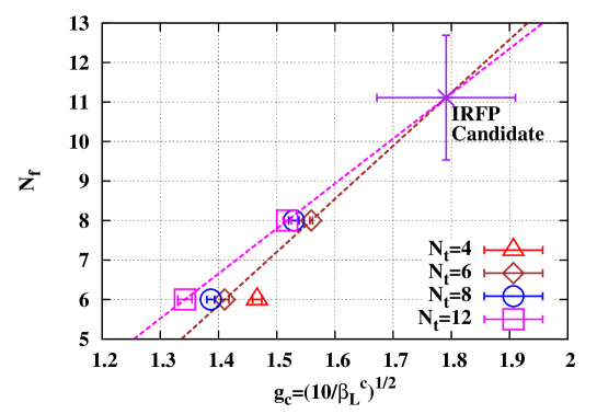
Figure 6: (Pseudo) critical values of the lattice coupling $g_{\mathrm{L}}^{~{}\mathrm{c}}=\sqrt{10/\beta_{\mathrm{L}}^{~{}\mathrm{c}}}$ for theories with $N_{f}=0,~{}4,~{}6,~{}8$ and for several values of $N_{t}$ in the Miransky-Yamawaki phase diagram. We have picked up $g_{\mathrm{L}}^{~{}\mathrm{c}}$ at $N_{f}=6$ and $8$, and considered “constant $N_{t}$” lines with $N_{t}=6,\ 12$. If the system is still described by one parameter beta-function in this range of coupling, the IRFP could be located at the intersection of the fixed $N_{t}$ lines – or equivalently, in the region where the step-scaling function vanishes. To demonstrate the procedure –as a preliminary example – we have considered the intersection of the $N_{t}=12$ and $N_{f}=6$ lines.

III.2 Towards the continuum limit: estimating again the conformal threshold

Let us now fix $N_{f}$ and consider the pseudo-critical temperatures $T_{c}$ in physical units:

$$T_{c}\equiv\frac{1}{a(\beta_{\mathrm{L}}^{~{}\mathrm{c}})\cdot N_{t}}\ .$$ (5)

We introduce the normalised critical temperature $T_{c}/\Lambda_{\mathrm{L/E}}$ (see e.g. Gupta:2000hr ) where $\Lambda_{\mathrm{L}}$ ($\Lambda_{\mathrm{E}}$) represents the lattice (E-scheme) Lambda-parameter defined in the two-loop perturbation theory with or without a renormalisation group inspired improvement CAllton .

We consider the two-loop beta-function

$$\beta(g)=-(b_{0}{g}^{3}+b_{1}{g}^{5})\ ,$$ (6)

$$b_{0}=\frac{1}{(4\pi)^{2}}\Biggl{(}\frac{11C_{2}[G]}{3}-\frac{4T[F]N_{f}}{3}\Biggr{)}\ ,$$ (7)

$$b_{1}=\frac{1}{(4\pi)^{4}}\Biggl{(}\frac{34(C_{2}[G])^{2}}{3}-\biggl{(}\frac{20C_{2}[G]}{3}+4C_{2}[F]\biggr{)}T[F]N_{f}\Biggr{)}\ ,$$ (8)

with $(C_{2}[G],\,C_{2}[F],\,T[F])=(N_{c},\,(N_{c}^{2}-1)/(2N_{c}),\,1/2)$. The coupling $g$ can be either the lattice bare coupling $g_{\mathrm{L}}=\sqrt{10/\beta_{\mathrm{L}}}$ or the E-scheme renormalised coupling $g_{\mathrm{E}}=\sqrt{3(1-\langle P\rangle(g_{\mathrm{L}}))}$, where $\langle P\rangle(g_{\mathrm{L}})$ is the zero temperature plaquette value. If the one-loop perturbation theory exactly holds, the E-scheme coincides the lattice scheme.

Integrating Eq. (6), we obtain the well-known two-loop asymptotic scaling relation,

$$R(g_{\mathrm{L/E}})\equiv a(g_{\mathrm{L/E}})\Lambda_{\mathrm{L/E}}=\bigl{(}b_{0}g_{\mathrm{L/E}}^{2}\bigr{)}^{-b_{1}/(2b_{0}^{2})}\exp\biggl{[}\frac{-1}{2b_{0}g_{\mathrm{L/E}}}\biggr{]}\ ,$$ (9)

where $\Lambda_{\mathrm{L}}$ ($\Lambda_{\mathrm{E}}$) is the Lattice (E-scheme) Lambda-parameter.

To take into account higher order corrections, we have also considered the renormalisation group inspired improvement CAllton

$$R^{\mathrm{imp}}(\beta_{\mathrm{L/E}})=\Lambda_{\mathrm{L/E}}^{\mathrm{imp}}~{}a(\beta_{\mathrm{L/E}})\equiv\frac{R(\beta_{\mathrm{L/E}})}{1+h}\times\Biggl{[}1+h\ \frac{R^{2}(\beta_{\mathrm{L/E}})}{R^{2}(\beta_{0})}\Biggr{]}\ ,$$ (10)

where $\beta_{\mathrm{L/E}}=10/(g_{\mathrm{L/E}})^{2}$. The coupling $\beta_{0}$ can be arbitrarily set and the parameter $h$ is adjusted so as to minimise the scaling violation. Note that $h=0$ reproduces the standard asymptotic scaling law Eq. (9).

We now substitute $\beta_{\mathrm{L/E}}^{~{}\mathrm{c}}$ into the temperature definition Eq. (5), and insert the scale $\Lambda_{\mathrm{L/E}}$:

$$\frac{1}{N_{t}}=\frac{T_{c}}{\Lambda_{\mathrm{L/E}}}\times\Bigl{(}\Lambda_{\mathrm{L/E}}~{}a(\beta_{\mathrm{L/E}}^{~{}\mathrm{c}})\Bigr{)}\ .$$ (11)

Eq. (11) allows us to define the (normalised) critical temperature $T_{c}/\Lambda_{\mathrm{L/E}}$. When we adopt the improvement Eq. (10), $T_{c}/\Lambda_{\mathrm{L/E}}$ is upgraded into $T_{c}/\Lambda_{\mathrm{L/E}}^{\mathrm{imp}}$.

$$\frac{T_{c}}{\Lambda_{\mathrm{L/E}}}=\frac{R(g_{\mathrm{L/E}})}{N_{t}}=\bigl{(}b_{0}g_{\mathrm{L/E}}^{2}\bigr{)}^{-b_{1}/(2b_{0}^{2})}\exp\biggl{[}\frac{-1}{2b_{0}}\biggr{]}\ ,$$ (12)

where $g_{\mathrm{L/E}}$ denotes either the bare lattice coupling or the coupling defined in the E scheme. In addition, we consider the renormalisation group inspired definition,

$$\frac{T_{c}}{\Lambda_{\mathrm{L/E}}^{\mathrm{imp}}}=\frac{R^{\mathrm{imp}}(g_{\mathrm{L/E}})}{N_{t}}\ ,$$ (13)

where $R^{\mathrm{imp}}$ is given by Eq. (10). The numerical results for $T_{c}/\Lambda_{\mathrm{L/E}}$ and $T_{c}/\Lambda_{\mathrm{L/E}}^{\mathrm{imp}}$ are collected in Table 2 and Table 3.

Table 2: Summary of $T_{c}/\Lambda_{\mathrm{L}}$ and $T_{c}/\Lambda_{\mathrm{L}}^{\mathrm{imp}}$ for various $(N_{f},N_{t})$. The first (second) line at fixed $(N_{f},N_{t})$ shows the value of $T_{c}/\Lambda_{\mathrm{L}}$ ($T_{c}/\Lambda_{\mathrm{L}}^{\mathrm{imp}}$), and the last two columns provide the parameter $h$ and $\beta_{0}$ appeared in the improved asymptotic scaling Eq. (10).

$N_{f}\backslash N_{t}$	$4$	$6$	$8$	$12$	$h$	$\beta_{0}$
$0$	$18.11\pm 0.65$	$18.21\pm 0.91$	$16.56\pm 0.71$	$-$	$-$	$-$
	$16.29\pm 0.75$	$17.81\pm 1.02$	$16.56\pm 0.78$	$-$	$0.05$	$8.26$
$4$	$21.99\pm 1.04$	$19.98\pm 0.95$	$17.12\pm 2.43$	$-$	$-$	$-$
	$16.56\pm 1.44$	$18.67\pm 1.38$	$17.12\pm 3.41$	$-$	$0.30$	$6.15$
$6$	$25.41\pm 1.43$	$25.33\pm 1.43$	$22.94\pm 1.29$	$22.30\pm 2.52$	$-$	$-$
	$21.66\pm 1.64$	$23.87\pm 1.58$	$22.21\pm 1.40$	$22.30\pm 2.66$	$0.03$	$5.55$
$8$	$-$	$50.05\pm 0.87$	$47.06\pm 3.28$	$34.34\pm 1.91$	$-$	$-$
	$-$	$34.32\pm 1.40$	$42.67\pm 6.33$	$34.34\pm 3.90$	$1.08$	$4.34$

Table 3: Summary of $T_{c}/\Lambda_{\mathrm{E}}$ and $T_{c}/\Lambda_{\mathrm{L/E}}^{\mathrm{imp}}$ for $N_{f}=6$ and $N_{f}=8$. The first (second) line at fixed $(N_{f},N_{t})$ shows the value of $T_{c}/\Lambda_{\mathrm{E}}$ ($T_{c}/\Lambda_{\mathrm{L/E}}^{\mathrm{imp}}$), and the last two columns give the parameter $h$ and $\beta_{0}$ appeared in the improved asymptotic scaling Eq. (10). For $N_{f}=6$, the improvement was not necessary.

$N_{f}\backslash N_{t}$	$4$	$6$	$8$	$12$	$h$	$\beta_{0}$
$6$	$74.22\pm 5.86$	$75.47\pm 8.17$	$74.56\pm 9.08$	$75.13\pm 10.76$	$-$	$-$
$8$	$-$	$422.54\pm 23.06$	$422.61\pm 38.59$	$316.03\pm 20.06$	$-$	$-$
	$-$	$312.16\pm 33.13$	$393.58\pm 60.01$	$316.03\pm 31.52$	$0.40$	$4.34$

Let us know consider the results at fixed $N_{f}$: for each $N_{f}$ , the ratio in either Table approaches a constant by increasing $N_{t}$, enabling us (with the due caveats) to interpret these asymptotic values as continuum estimates.

Let us then take the values corresponding to the largest $N_{t}$ and consider their $N_{f}$ dependence : $T_{c}/\Lambda$ apparently increases with $N_{f}$! How this can be reconciled with a vanishing $T_{c}$ in the chiral limit? This is discussed below, and again in the last Section.

III.3 The critical number of flavor and the vanishing critical temperature

The apparent puzzle above immediately suggests that $\Lambda$ vanishes faster than $T_{c}$ when approaching $N_{f}$, i.e. has a strong sensitivity to the IR dynamics affected by the conformal threshold.

To observe the vanishing of $T_{c}$ we then need to properly define a UV reference scale. Here we will review our first attempt to do so which relies heavily on perturbation theory, while in the last Section we will describe our ongoing work on this subject.

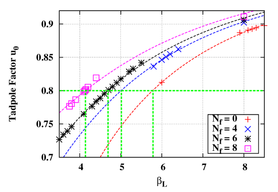
Figure 7: The $\beta_{\mathrm{L}}$ dependence of the tadpole factor $u_{0}$ at zero temperature ($12^{4}$ lattice volume). At each $N_{f}$, the dashed line represents the fit for data with the ansatz $u_{0}=1-A/(1+B\cdot\beta_{\mathrm{L}}^{2})$. We consider a constant $u_{0}$ (e.g. $u_{0}=0.8$ in figure), and read off the corresponding lattice bare couplings $\beta_{\mathrm{L}}$, which are used to define the scale $M$ at each theory with $N_{f}$ flavors.

Before going to details, we first explain the basic idea which follows the FRG analysis by Braun and Gies BraunGies . They used the $\tau$ lepton mass $m_{\tau}=1.777$ (GeV) as an $N_{f}$ independent UV reference scale for theories with any number of flavors. The initial condition of the renormalisation flow has been specified via the strong coupling constant in an $N_{f}$ independent way:

$$\alpha_{s}(\mu=m_{\tau})=0.322\quad\text{for}\quad{}^{\forall}N_{f}\ .$$ (14)

Starting from the common initial condition Eq. (14), the $N_{f}$ dependence of the critical temperature $T_{c}(N_{f})$ emerges from the $N_{f}$ dependent renormalisation flow at the chiral phase transition scale $\mu\sim\Lambda_{\mathrm{QCD}}\ll m_{\tau}$.

The $N_{f}$ dependence of $T_{c}$ as well as its novel non-analytic behaviour in the pre-conformal region becomes free from the choice of the reference scale BraunGies by using an $N_{f}$ independent UV reference scale much larger than $T_{c}$.

In order to determine the reference coupling $g_{\mathrm{L}}^{~{}\mathrm{ref}}$ we utilise our plaquette results $\langle P\rangle$ (equivalently, the tadpole factor $u_{0}=\langle P\rangle^{1/4}$) shown in Fig. 7.

Let us consider a constant $u_{0}$, for instance $u_{0}=0.8$ in figure, and read off the corresponding bare lattice couplings at each $N_{f}$. The obtained $g_{\mathrm{L}}(N_{f})$ is used as a reference coupling $g_{\mathrm{L}}^{~{}\mathrm{ref}}$ and the corresponding mass scale $M(g_{\mathrm{L}}^{~{}\mathrm{ref}})$ is again computed according to two loop scaling.

Some remarks on the aforementioned scale setting are in order: First, we recall the scale setting procedure in the potential scheme, where the measured normalised force $r^{2}F(r)$ is proportional to the renormalised coupling $\bar{g}$, and the specification $\bar{g}^{2}\propto r_{X}^{2}F(r_{X})={}^{\exists}X$ sets a scale $r_{X}^{-1}$. In short, we use our $u_{0}$ (or equivalently plaquettes) to define $\bar{g}$, and $u_{0}=X$ is regarded as the analog of the potential scheme scale setting. Second, in the leading order of the perturbative expansion, the renormalised coupling is $N_{f}$ independent, and proportional to the Wilson loop Wong:2005jx – a property that we have already exploited in the E-scheme calculation. Hence the use of an $N_{f}$ independent $u_{0}$ approximately gives an $N_{f}$ independent scale setting, similarly to the FRG scale setting method Eq. (14). And third, such an $N_{f}$ independent scale setting can be performed in a sufficiently UV regime $T_{c}(N_{f})\ll M(g_{\mathrm{L}}^{~{}\mathrm{ref}})$ by adjusting the value of $u_{0}$ to satisfy the condition $g_{\mathrm{L}}^{~{}\mathrm{ref}}\ll g_{\mathrm{T}}^{~{}\mathrm{c}}({}^{\forall}N_{f})$.

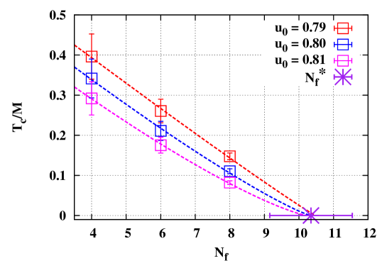
Figure 8: Left:  The $N_{f}$ dependence of $T_{c}/M$ where $M$ is determined to be a UV scale corresponding to $u_{0}=0.79$ (red box), $0.80$ (blue $\bigcirc$), and $0.81$ (magenta triangle) at each theory with $N_{f}$. The dashed lines represent fits for data by assuming the expression Eq. (15)

Note that the coupling at the lattice cutoff $a^{-1}(g_{\mathrm{L}}^{~{}\mathrm{c}})$ is $N_{t}\gg 1$ times larger than $T_{c}$. Then, the scale hierarchy $T_{c}(N_{f})\ll a^{-1}(g_{\mathrm{L}}^{~{}\mathrm{c}}(N_{f}))$ allows us to consider a reference scale much larger than critical temperature but smaller than the lattice cutoff $T_{c}(N_{f})\ll M(g_{\mathrm{L}}^{~{}\mathrm{ref}})<a^{-1}(g_{\mathrm{L}}^{~{}\mathrm{c}}(N_{f}))$. We find that $u_{0}\sim 0.8$ meets this requirement.

In summary, the use of $g_{\mathrm{L}}^{~{}\mathrm{ref}}$ given by $u_{0}\sim 0.8$ is analogous to the FRG scale setting method Eq. (14), and is suitable for studying the vanishing of the critical temperature by utilising $T_{c}/M(g_{\mathrm{L}}^{~{}\mathrm{ref}})$.

Fig. 8 displays the $N_{f}$ dependence of $T_{c}/M(g_{\mathrm{L}}^{~{}\mathrm{ref}})$ for $u_{0}=0.79$, $0.80$, and $0.81$. Fitting the data points for $T_{c}/M(g_{\mathrm{L}}^{~{}\mathrm{ref}})$ at $N_{f}\geq 4$ by using the FRG motivated ansatz,

$$T_{c}=K|N_{f}^{*}-N_{f}|^{(-2b_{0}^{2}/b_{1})(N_{f}^{*})}\ ,$$ (15)

where $b_{0,1}$ has been defined in Eqs. (7) and (8), the lower edge of the conformal window is estimated as: $N_{f}^{*}=10.48\pm 1.01$ ($u_{0}=0.79$), $N_{f}^{*}=10.34\pm 0.88$ ($u_{0}=0.80$), $N_{f}^{*}=10.23\pm 0.80$ ($u_{0}=0.81$). The error-bars involve both fit errors and statistical errors of data.

We have further investigated the stability against different choices of $u_{0}$: $N_{f}^{*}$ is relatively stable within the range $0.79\leq u_{0}\leq 0.94$. The scale cannot be pushed further towards the UV because of discritization errors. On the other hand, a small $u_{0}\lesssim 0.7$ leads to $M(g_{\mathrm{L}}^{~{}\mathrm{ref}})\sim T_{c}$ or smaller. In such a case, the reference scale $M(g_{\mathrm{L}}^{~{}\mathrm{ref}})$ is affected by infra-red physics and cannot be used to study the vanishing of $T_{c}$. Despite these limitations, the window of relative stability is however reasonably large, and suffices to define an average value for $N_{f}^{*}$. We quote the average among the three results obtained for $u_{0}=(0.79,0.80,0.81)$, i.e. $N_{f}^{*}=10.4\pm 1.2$.

IV Learning about the Quark Gluon Plasma when studying the threshold for conformality

In this second subsection, we will follow the approach of a recent paper Liao:2012tw , and compute the coupling $g_{\mathrm{T}}^{~{}\mathrm{c}}(N_{f})$ at the scale of the critical temperature for each $N_{f}$. To obtain the coupling $g_{\mathrm{T}}^{~{}\mathrm{c}}$ at the scale of the temperature, we evolve the coupling at the scale of the lattice spacing $a$ up to the temperature inverse scale $N_{t}a$, still making use of the two loop scaling, which, as we have seen, is reasonably well satisfied.

The red ($\Box$) symbol in Fig. 9 shows $g_{\mathrm{T}}^{~{}\mathrm{c}}$ as a function of $N_{f}$. We superimpose a fit obtained by using the ansatz proposed in Ref. Liao:2012tw

$${N_{f}(g_{\mathrm{T}}^{~{}\mathrm{c}})=A\cdot\log~{}\bigl{[}B\cdot(g_{\mathrm{T}}^{~{}\mathrm{c}}-g_{\mathrm{T}}^{~{}\mathrm{c}}|_{N_{f}=0})+1\bigr{]}\ .}$$ (16)

with $A$ and $B$ fit parameters, which describes well the data.

Since the critical temperature is zero in the conformal phase, the thermal critical coupling $g_{\mathrm{T}}^{~{}\mathrm{c}}$ should equal a zero temperature critical coupling $g^{c}$ when $N_{f}=N_{f}^{*}$. Of course, $g^{c}$ is not known exactly and we have to rely on approximations.

The first estimate is based on the best available value $g_{\mathrm{SD}}^{\mathrm{c}}$ obtained by using the two-loop Schwinger-Dyson equation Appelquist . In this case, the lower edge of the conformal window $N_{f}^{*}$ is defined by the condition $g_{\mathrm{T}}^{~{}\mathrm{c}}(N_{f}^{*})=g_{\mathrm{SD}}^{\mathrm{c}}(N_{f}^{*})$. In Fig. 9 $g_{\mathrm{SD}}^{\mathrm{c}}$ is plotted as a blue solid line. We then estimate the intersection of $g_{\mathrm{T}}^{~{}\mathrm{c}}$ and $g_{\mathrm{SD}}^{\mathrm{c}}$ – hence the onset of the conformal window as well as the IRFP coupling at $N_{f}^{*}$ – at $(g^{*},N_{f}^{*})=(2.79,13.2)\pm(0.13,0.6)$.

One second possibility for estimating $N_{f}^{*}$ is the following: the conformal phase would emerge when the coupling at IRFP ($g^{\mathrm{IRFP}}$) is not strong enough to break chiral symmetry, i.e. $g^{\mathrm{IRFP}}\leq g_{\mathrm{T}}^{~{}\mathrm{c}}$. Here, we utilise the four-loop result for $g_{\mathrm{4l}}^{\mathrm{IRFP}}$ Ryttov:2012nt as the best available. In Fig. 9, we show $g_{\mathrm{4l}}^{\mathrm{IRFP}}$ as magenta $\bigcirc$, with superimposed a linear interpolation. In the plot, we use the results for $g_{\mathrm{4l}}^{\mathrm{IRFP}}$ in the $\bar{\text{MS}}$ scheme. The errors are estimated by considering the scheme dependence Ryttov:2012nt , which turns out to be rather mild at four loops. We can then locate the intersection of $g_{\mathrm{T}}^{~{}\mathrm{c}}$ and $g_{\mathrm{4l}}^{\mathrm{IRFP}}$ and obtain $(g^{*},N_{f}^{*})=(2.51,11.8)\pm(0.15,0.9)$.

Ideally, the three lines in Fig. 9 should meet at a (single) IRFP fixed point, if all the quoted results – including the analytic ones – were exact. Indeed the intersections we have estimated are consistent within the largish errors. We then quote the average of the above two estimates as our final result from this analysis, $N_{f}^{*}\sim 12.5\pm 1.6$.

In addition, we note that $g_{\mathrm{T}}^{~{}\mathrm{c}}$ is an increasing function of $N_{f}$. This indicates that the quark-gluon plasma is more strongly coupled at larger $N_{f}$, as discussed in Ref. Liao:2012tw . In turn, this observation might provide a clue into the nature of the strongly interactive quark gluon plasma.

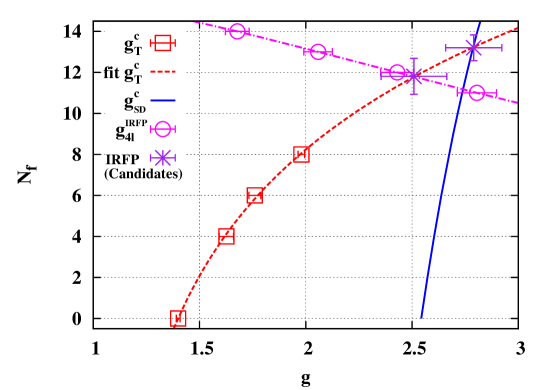
Figure 9: The thermal critical coupling (red $\Box$) and the fit for them (dashed red line, with the ansatz Eq. (16)) and the values of the zero temperature couplings in the conformal phase from different estimates, see text for details. At the critical number of flavor the thermal critical coupling should equal the critical coupling associated with the IRFP. The procedure is motivated by a recent study by Shuryak in Ref. Liao:2012tw .

V Two scales?

Let us elaborate on the circumstance that $T_{c}/\Lambda$ computed using different schemes ($\Lambda=\Lambda_{\mathrm{L}}$ or $\Lambda_{\mathrm{E}}$) consistently shows an increase with $N_{f}$, as initially noted in Miura:2011mc . As discussed in Miura:2011mc this indicates that $\Lambda_{\mathrm{L/E}}$ vanishes faster than $T_{c}$ upon approaching the critical number of flavor. Within the various uncertainties discussed here, this can be taken as a qualitative indication of scale separation close to the critical number of flavors.

In the Section above, we have estimated the onset of the conformal phase $N^{∗}_{f}$ via the vanishing of $T_{c}(N_{f})/M$. As a next step, it is preferable to define $T_{c}(N_{f})/M$ without recourse to perturbation theory.

To this end, we have adopted the string tension $\sigma$ as a reference scale $M$, and investigated $T_{c}/\sqrt{\sigma}$ (Fig. 10). The $\sigma$ is evaluated from the Wilson loop measured on zero temperature lattices, for the same set of pseudocritical couplings we have identified in our thermal study. The $T_{c}/\sqrt{\sigma}$ remains stable in the error, again suggesting that our results are a reasonable approximation of the continuum ones.

$T_{c}/\sqrt{\sigma}$ = 0.373(2)(+5,-6) (0.369(4)(+1,-5)) for $N_{f}=6(8)$, and the decreasing trend becomes less apparent with increasing $N_{f}$ , and $T_{c}/\sqrt{\sigma}$ does not seem to intercept the $N_{f}$ axis before the asymptotic freedom is lost ($N_{f}=16.5$). This may not be surprising. We find at least two reasons for the non-vanishing $T_{c}/\sqrt{\sigma}$ : First, $\sigma$ would not be a “UV” quantity and may also be vanishing when a conformal phase sets in. In other words, our result indicates that the regulator of $T_{c}$ has to be more UV than $\sigma$ to elucidate the vanishing of chiral symmetry breaking via $T_{c}$ . From this point of view, a quantity $T_{c}w_{0}$ where $w_{0}$ is a UV scale Borsanyi:2012zs defined by the Wilson flow Luscher:2009eq may be a candidate which we are currently evaluating. Suppose $T_{c}w_{0}$ displayed the expected hints of singularity at our estimated $N_{f}^{*}$: our estimate of the critical number of flavor would be confirmed, and we will have a significant evidence of a scale separation - the two different scales bing $\sigma$ and $w_{0}$. Again however one might argue that a finite bare fermion mass breaks the conformality, and both $T_{c}$ and $\sigma$ could be defined and finite even in the region $N_{f}\geq N^{∗}_{f}$. Thus bare fermion mass effects to $T_{c}/\sqrt{\sigma}$ should be further studied in future.

As indicated in Ref. Gursoy:2010fj , the ratio $T_{c}/\sqrt{\sigma}$ is one of the input parameters to set a scale in models based on the gauge/gravity duality at finite T. Such inputs for the (would-be) walking regime $N_{f}=6$ and $N_{f}=8$ are now available by the present study.

A final caveat concerns the occurrence of a small oscillatory behavior in the effective mass of the Wilson loop with smearing for $N_{f}=8$. It remains to be seen how these oscillations relate to the bulk transition observed in the conformal window: for instance these observations might confirm the original scenario in which the bulk transition would still manifest itself in the QCD phase, as a (pseudo)singularity unrelated with the chiral transition.

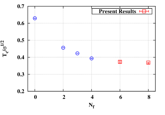
Figure 10: The $T_{c}/\sqrt{\sigma}$ as a function of $N_{f}$. The symbol $\Box$ (red) represents the present results ($N_{f}=6,8$). For a comparison, we have quoted the $T_{c}/\sqrt{\sigma}$ from Laermann:1996xn ($N_{f}=0$), Karsch:2000kv ($N_{f}=2,3$), Engels:1996ag ($N_{f}=4$), shown as $\bigcirc$ (blue) symbols.

VI Summary

We have presented an overview of some of our results on the phases of QCD at large number of flavor $N_{f}$, with some emphases on the scales of the theory, and on the scale setting procedure: oversimplifying, QCD generates one dynamically relevant scale for a small number of flavors, becomes a multi-scale theory when approaching the conformal window, and then looses its infra red scale.

We need consistent procedures of scale setting in order to properly appreciate these phenomena. We are confident that we have taken at least some steps towards this goal and we hope that the strategies we have developed will help further sharpen some of the still semi-quantitative estimates presented here.

For $N_{f}=12$, our measurements of the order parameter and of the spectrum to our results provide evidence towards the existence of a symmetric, Coulomb-like phase on the weak coupling side of the lattice bulk transition. In the scenario of Refs. Appelquist ; Miransky:1997 , such a Coulomb-like region must be entangled to the presence of a conformal IRFP for the theory with twelve flavors at a continuum limit. We have then analyzed the spectrum results as a function of mass, and found them to be well described by power-law fits with a mass anomalous dimension consistent with other lattice results and as well as the analytic estimates Itou:2013ofa .

On the QCD side ($N_{f}<N_{f}^{*}$), we have investigated the chiral phase transition/crossover with $N_{f}=0$ (quenched), $4$, $6$, and $8$. We have discussed the possible implication for the (pre-)conformal dynamics at large $N_{f}$, and estimated, in a few independent ways, the number of flavor $N_{f}^{*}$: We have estimated the $N_{f}^{*}$ from the vanishing thermal scaling by extrapolating our critical couplings $g_{\mathrm{L}}^{~{}\mathrm{c}}$ to larger $N_{f}$ . This gives $N_{f}^{*}\sim 11.1\pm 1.6$. We have extracted a typical interaction strength $g_{\mathrm{T}}^{~{}\mathrm{c}}$ at the scale of critical temperature $T_{c}$ by utilising our $g_{\mathrm{L}}^{~{}\mathrm{c}}$ and the two-loop beta-function, and compared $g_{\mathrm{T}}^{~{}\mathrm{c}}$ to the zero temperature critical couplings ($g_{\mathrm{SD}}^{\mathrm{c}}$) estimated by the two-loop Schwinger-Dyson equation Appelquist as well as the IRFP position ($g_{\mathrm{4l}}^{\mathrm{IRFP}}$) of the four-loop beta-function Ryttov:2012nt . The coincidence between $g_{\mathrm{T}}^{~{}\mathrm{c}}$ and $g_{\mathrm{SD}}^{\mathrm{c}}$ or $g_{\mathrm{4l}}^{\mathrm{IRFP}}$ indicates the vanishing critical temperature with the emergence of the conformal phase. Based on this reasoning, we have estimated the onset of the conformal window as $N_{f}^{*}\sim 12.5\pm 1.6$. We have also confirmed the increasing of $g_{\mathrm{T}}^{~{}\mathrm{c}}$ at larger $N_{f}$ which has been discussed in Ref. Liao:2012tw and indicates more strongly interacting non-Abelian plasma at larger $N_{f}$.

Further, we have examined the $N_{f}$ dependence of $T_{c}/M$ for a variety of choices for a reference scale $M$: we have first considered a UV reference scale $M$ which is determined by utilising the tadpole factor $u_{0}$. Then, $T_{c}/M$ turns out to be a decreasing function of $N_{f}$ consistently to the FRG observations BraunGies , and the vanishing $T_{c}/M$ indicates the emergence of the conformal window around $N_{f}^{*}\sim 10.4\pm 1.2$.

Then we have studied $T_{c}/\sqrt{\sigma}$ and we are currently extending our study to $T_{c}w_{0}$ : the comparison among these different scale setting procedures allows a controlled observation of the genuine singularities - if any - associated with the onset of conformality, and should highlight the emergence of different scales in the pre-conformal window.

Last but not the least, we expect that our thermodynamic lattice study for the large $N_{f}$ non-Abelian gauge theory plays an important role as a new connection between the lattice and the Gauge/Gravity duality Gursoy:2010fj ; Alho:2012mh .

VII Acknowledgments

MPL and KM were partially supported by the PRIN ‘Frontiers of Strong Interactions’ funded by the MIUR. This work was in part based on the MILC Collaboration’s public lattice gauge theory code MILC . The numerical calculations for the chiral phase transition BG/P at CINECA in Italy and the Hitachi SR-16000 at YITP, Kyoto University in Japan. The numerical calculations for making the gauge configurations at zero temperature were performed in BG/Q at CINECA in Italy. The Wilson loop measurements were carried out on the high-performance computing system ϕ at KMI, Nagoya University in Japan. We wish to thank Marc Wagner for providing us the code for the Wilson loop measurements.

Note added : After the acceptance of this work we have completed our paper On the particle spectrum and the conformal windowLombardo:2014pda , which addresses the open issues of Section II providing a nonperturbative determination of the fermion mass anomalous dimension $\gamma=0.235(46)$.

References

- (1) The reader might want to consult the proceedings of the conferences Strong Coupling Gauge Theories, Nagoya, 2009, and 2012 for comprehensive background material.
- (2) For an introduction see e.g. F. Sannino, “Conformal Dynamics for TeV Physics and Cosmology,” Acta Phys. Polon. B 40 (2009) 3533.
- (3) K. Yamawaki, M. Bando and K. -i. Matumoto, Phys. Rev. Lett. 56 (1986) 1335.
- (4) B. Holdom, Phys. Lett. B 150, 301 (1985).
- (5) T. Akiba and T. Yanagida, Phys. Lett. B 169, 432 (1986).
- (6) T. W. Appelquist, D. Karabali and L. C. R. Wijewardhana, Phys. Rev. Lett. 57, 957 (1986).
- (7) J. Kuti, PoS LATTICE 2013 (2013) 004.
- (8) J. Giedt, PoS LATTICE2012 (2012) 006.
- (9) L. Del Debbio, PoS LATTICE2010 (2010) 004.
- (10) E. Pallante, PoS LATTICE2009 (2009) 015.
- (11) Both lattice and analytic results on the mass anomalous dimension are summarized in the recent lattice review, E. Itou, arXiv:1311.2998 [hep-lat].
- (12) T. Appelquist, G. T. Fleming, M. F. Lin, E. T. Neil, D. A. Schaich, Phys. Rev. D84, 054501 (2011).
- (13) T. Appelquist, G. T. Fleming and E. T. Neil, Phys. Rev. D 79 (2009) 076010.
- (14) T. Appelquist et al., Phys. Rev. Lett. 104 (2010) 071601.
- (15) T. Appelquist et al. [ LSD Collaboration ], Phys. Rev. Lett. 106 (2011) 231601.
- (16) A. Deuzeman, M. P. Lombardo and E. Pallante, Phys. Lett. B 670 (2008) 41.
- (17) A. Deuzeman, M. P. Lombardo and E. Pallante, Phys. Rev. D 82 (2010) 074503.
- (18) A. Deuzeman, M. P. Lombardo, T. Nunes Da Silva and E. Pallante, Phys. Lett. B 720 (2013) 358.
- (19) A. Deuzeman, M. P. Lombardo and E. Pallante, PoS LATTICE 2011 (2011) 083.
- (20) K. Miura, M. P. Lombardo and E. Pallante, Phys. Lett. B 710 (2012) 676.
- (21) K. Miura and M. P. Lombardo, Nuclear Physics B 871 (2013) 52.
- (22) Y. Aoki et al. [the LatKMI Collaboration], Phys. Rev. D 89 (2014) 111502.
- (23) Y. Aoki et al. [LatKMI Collaboration], Phys. Rev. Lett. 111 (2013) 16, 162001.
- (24) Y. Aoki et al. [LatKMI Collaboration], Phys. Rev. D 87 (2013) 9, 094511.
- (25) Y. Aoki, T. Aoyama, M. Kurachi, T. Maskawa, K. -i. Nagai, H. Ohki, A. Shibata and K. Yamawaki et al., Phys. Rev. D 86 (2012) 054506.
- (26) A. Cheng, A. Hasenfratz, Y. Liu, G. Petropoulos and D. Schaich, JHEP 1405 (2014) 137 [arXiv:1404.0984 [hep-lat]].
- (27) A. Cheng, A. Hasenfratz, G. Petropoulos and D. Schaich, JHEP 1307 (2013) 061.
- (28) A. Cheng, A. Hasenfratz and D. Schaich, Phys. Rev. D 85 (2012) 094509.
- (29) A. Hasenfratz, Phys. Rev. Lett. 108 (2012) 061601.
- (30) A. Hasenfratz, Phys. Rev. D 82 (2010) 014506.
- (31) A. Hasenfratz, Phys. Rev. D 80 (2009) 034505.
- (32) Z. Fodor, K. Holland, J. Kuti, D. Nogradi and C. Schroeder, Phys. Lett. B703 (2011) 348-358.
- (33) Z. Fodor, K. Holland, J. Kuti, D. Nogradi and C. Schroeder, Phys. Lett. B 681 (2009) 353.
- (34) K. -I. Ishikawa, Y. Iwasaki, Y. Nakayama and T. Yoshie, Phys. Rev. D 89 (2014) 114503.
- (35) K. -I. Ishikawa, Y. Iwasaki, Y. Nakayama and T. Yoshie, Phys. Rev. D 87 (2013) 7, 071503.
- (36) Y. Iwasaki, K. Kanaya, S. Kaya, S. Sakai and T. Yoshie, Phys. Rev. D 69 (2004) 014507.
- (37) T. Karavirta, A. Mykkanen, J. Rantaharju, K. Rummukainen and K. Tuominen, JHEP 1106 (2011) 061.
- (38) Y. Shamir, B. Svetitsky and E. Yurkovsky, Phys. Rev. D 83 (2011) 097502.
- (39) J. B. Kogut and D. K. Sinclair, Phys. Rev. D 81 (2010) 114507.
- (40) Z. Fodor, K. Holland, J. Kuti, D. Nogradi and C. Schroeder, JHEP 0911 (2009) 103.
- (41) Z. Fodor, K. Holland, J. Kuti, D. Nogradi, C. Schroeder and C. H. Wong, Phys. Lett. B 718 (2012) 657.
- (42) S. Catterall, J. Giedt, F. Sannino and J. Schneible, JHEP 0811 (2008) 009.
- (43) L. Del Debbio, B. Lucini, A. Patella, C. Pica and A. Rago, Phys. Rev. D 82 (2010) 014510.
- (44) L. Del Debbio and R. Zwicky, Phys. Lett. B 700 (2011) 217.
- (45) L. Del Debbio and R. Zwicky, Phys. Rev. D 82 (2010) 014502.
- (46) Ph. de Forcrand, S. Kim and W. Unger, JHEP 1302 (2013) 051.
- (47) J. Braun, C. S. Fisher, H. Gies, Phys. Rev. D84 (2011) 034045.
- (48) M. Jarvinen and E. Kiritsis, JHEP 1203 (2012) 002.
- (49) T. Alho, M. Järvinen, K. Kajantie, E. Kiritsis and K. Tuominen, JHEP 1301 (2013) 093.
- (50) U. Gursoy, E. Kiritsis, L. Mazzanti, G. Michalogiorgakis and F. Nitti, Lect. Notes Phys. 828 (2011) 79.
- (51) T. Alho, N. Evans and K. Tuominen, Phys. Rev. D 88 (2013) 105016 [arXiv:1307.4896 [hep-ph]].
- (52) J. Liao, E. Shuryak and E. Shuryak, Phys. Rev. Lett. 109, 152001 (2012).
- (53) T. A. Ryttov and R. Shrock, Phys. Rev. D 86 (2012) 085005.
- (54) T. A. Ryttov and F. Sannino, Phys. Rev. D 78 (2008) 065001.
- (55) D. D. Dietrich and F. Sannino, Phys. Rev. D 75 (2007) 085018.
- (56) O. Antipin, M. Mojaza and F. Sannino,O. Antipin, M. Mojaza and F. Sannino, Phys. Rev. D 87 (2013) 9, 096005.
- (57) S. Matsuzaki and K. Yamawaki, arXiv:1311.3784 [hep-lat].
- (58) S. Matsuzaki and K. Yamawaki, Phys. Rev. D 86 (2012) 115004.
- (59) W. E. Caswell, Phys. Rev. Lett. 33 (1974) 244.
- (60) T. Banks and A. Zaks, Nucl. Phys. B 196 (1982) 189.
- (61) V. A. Miransky and K. Yamawaki, Phys. Rev. D 55 (1997) 5051 [Erratum-ibid. D 56 (1997) 3768].
- (62) T. Appelquist, J. Terning and L. C. R. Wijewardhana, Phys. Rev. Lett. 77 (1996) 1214.
- (63) T. Appelquist, A. G. Cohen and M. Schmaltz, Phys. Rev. D 60 (1999) 045003.
- (64) V. A. Novikov, M. A. Shifman, A. I. Vainshtein and V. I. Zakharov, Nucl. Phys. B 229, 381 (1983).
- (65) M. Velkovsky and E. V. Shuryak, Phys. Lett. B 437 (1998) 398.
- (66) R. D. Pisarski and F. Wilczek, Phys. Rev. D 29 (1984), 338.
- (67) A. Kocic, J. B. Kogut and M. -P. Lombardo, Nucl. Phys. B 398 (1993) 376.
- (68) S. Gupta, Phys. Rev. D 64 (2001) 034507.
- (69) C. R. Allton, Nucl. Phys. Proc. Suppl. 53 (1997) 867.
- (70) K. Y. Wong, H. D. Trottier and R. M. Woloshyn, Phys. Rev. D 73 (2006) 094512.
- (71) J. B. Kogut, J. Polonyi, H. W. Wyld and D. K. Sinclair, Phys. Rev. Lett. 54, 1475 (1985).
- (72) P. H. Damgaard, U. M. Heller, A. Krasnitz and P. Olesen, Phys. Lett. B 400 (1997) 169.
- (73) S. Borsanyi, S. Durr, Z. Fodor, C. Hoelbling, S. D. Katz, S. Krieg, T. Kurth and L. Lellouch et al., JHEP 1209 (2012) 010.
- (74) M. Luscher, Commun. Math. Phys. 293 (2010) 899.
- (75) E. Laermann, Nucl. Phys. A 610 (1996) 1C.
- (76) F. Karsch, E. Laermann and A. Peikert, Nucl. Phys. B 605 (2001) 579.
- (77) J. Engels, R. Joswig, F. Karsch, E. Laermann, M. Lutgemeier and B. Petersson, Phys. Lett. B 396 (1997) 210.
- (78) MILC Collaboration, http://www.physics.indiana.edu/~sg/milc.html
- (79) M. P. Lombardo, K. Miura, T. J. N. da Silva and E. Pallante, arXiv:1410.0298 [hep-lat].