Autoresonant control of the magnetization switching in single-domain nanoparticles

Abstract

The ability to control the magnetization switching in nanoscale devices is a crucial step for the development of fast and reliable techniques to store and process information. Here we show that the switching dynamics can be controlled efficiently using a microwave field with slowly varying frequency (autoresonance). This technique allowed us to reduce the applied field by more than $30\%$ compared to competing approaches, with no need to fine-tune the field parameters. For a linear chain of nanoparticles the effect is even more dramatic, as the dipolar interactions tend to cancel out the effect of the temperature. Simultaneous switching of all the magnetic moments can thus be efficiently triggered on a nanosecond timescale.

I Introduction

The fast and reliable control of the magnetization dynamics in magnetic materials has been a topical area of research for the last two decades. In particular, single-domain magnetic nanoparticles have attracted much attention, both for fundamental research on nanoscale magnetism and for potential technological applications to magnetic data storage, which is expected to increase to several petabit/inch² (10${}^{15}\rm cm^{-2})$ in the near future weller ; Gubin . For the fast processing and retrieval of the stored information, a precise control of the magnetization switching dynamics is a necessary requirement Hillebrands ; Back ; Gerrits ; Schumacher ; Seki . Single-domain nanoparticles with uniaxial anisotropy possess two stable orientations of the magnetic moment along the anisotropy axis, separated by an energy barrier proportional to the volume of the particle. This feature renders them particularly attractive as information-storage units. However, for very small particles the barrier can be of the same order as the temperature, so that the magnetic moment switches randomly between the two orientations under the effect of the thermal fluctuations weller1 , thus precluding any fine control of the magnetization dynamics. This phenomenon is known as superparamagnetism.

A potential solution would be to use nanoparticles with high magnetic anisotropy Sun . But an increased anisotropy requires larger fields to reverse the magnetization of the nanoparticle, which is currently difficult to achieve experimentally and causes unwanted noise. In order to elude this limitation, a microwave field can be combined to the static field chang ; miltat . For cobalt nanoparticles, it was shown that a monochromatic microwave field can significantly reduce the static switching field thirion and that the optimal field should be modulated both in frequency and amplitude using a feedback technique barros . However, the use of such a feedback mechanism can be costly and cumbersome in practical situations. Some authors also pointed out that the onset of chaos in the magnetization dynamics can facilitate the reversal of the magnetic moment daquino .

Here, we propose a more effective technique that relies on the concept of autoresonance. This approach was originally devised for a simple nonlinear oscillator (e.g., a pendulum) driven by a chirped force with a slowly varying frequency fajans01 ; peinetti ; marcus . If the driving amplitude exceeds a certain threshold, then the nonlinear frequency of the oscillator stays locked to the excitation frequency, so that the resonant match is never lost (until, of course, some other effects start to kick in). Importantly, the autoresonant excitation requires no fine-tuned feedback mechanism.

Autoresonant excitation has been observed in a wide variety of environments, including atomic systems meerson ; liu , plasmas fajans99a ; fajans99b , fluids friedland99 , and semiconductor quantum wells manfredi . Some authors also noticed the beneficial effect of a chirped pulse on the magnetization dynamics in a nanoparticle cai ; wang ; Rivkin , but lacked the analytical tools provided by the autoresonance theory. The autoresonance theory was used in the past to study the excitation of high-amplitude magnetization precession in ferromagnetic thin films Shamsutdinov and the dynamics of localized magnetic inhomogeneities in a ferromagnet Kalyakin . However, those authors did not investigate realistic physical systems and their analysis remained very abstract.

In the present work, we concentrate on a specific physical system that has long been studied experimentally in the past thirion , namely single-domain magnetic nanoparticles. We will show how the autoresonant mechanism can be fully exploited to control the magnetization reversal dynamics in a coherent fashion, on a timescale of a few tens of nanoseconds. Although this is longer that the picosecond switching time that can be achieved in principle with all-optical techniques Rasing , the latter require the use of finely tailored laser pulses and are thus more complex to implement in practice.

Our analysis takes into account, within the framework of the macrospin approximation, the majority of important physical mechanisms, such as the temperature (which is deleterious for the coherent control) and the dipolar interactions between nanoparticles (which turn out to favor coherent switching). With the proposed method, we are able to reduce the switching field by more than 30% compared to competing microwave approaches, with no need to fine-tune the field parameters.

II Model

Our treatment can be applied to a variety of physical systems that can be described by a macroscopic magnetization (macrospin). As a concrete example, we consider an isolated magnetic nanoparticle with uniaxial anisotropy along $\mathbf{e}_{z}$ in the macrospin approximation ($\lvert\mathbf{M}\rvert$ is constant), in the presence of an external static field collinear to the anisotropy axis . An oscillating AC microwave field of varying frequency will constitute the autoresonant excitation. The adopted configuration is sketched on Fig. 1.

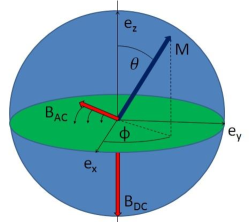
Figure 1: Color online. Geometric configuration of the nanoparticle with its magnetic moment ${\mathbf{M}}(\theta,\phi)$, the static field $\mathbf{B}_{DC}$, and the time-dependent AC field $\mathbf{B}_{AC}(t)$. The case of an AC field rotating in the $(\mathbf{e}_{x},\mathbf{e}_{y})$ plane is shown on the figure.

The evolution of the macroscopic moment $\mathbf{M}=\mu_{S}\mathbf{m}$, of constant amplitude $\mu_{S}$ and direction along $\mathbf{m}$, is governed by the Landau-Lifshitz-Gilbert (LLG) equation:

$${\frac{d\mathbf{M}}{dt}}=-{\frac{\gamma}{(1+\lambda^{2})}}(\mathbf{M}\times\mathbf{B}_{eff})\\ -{\frac{\gamma\lambda}{(1+\lambda^{2})\mu_{S}}}[\mathbf{M}\times(\mathbf{M}\times\mathbf{B}_{eff})],$$ (1)

where $\gamma=1.76\times 10^{11}~{}\rm(Ts)^{-1}$ is the gyromagnetic ratio, $\lambda=0.01$ the phenomenological damping parameter in the weak damping regime, and $\mathbf{B}_{eff}$ the effective field acting on the particle. The latter is the sum of the anisotropy field $\mathbf{B}_{an}=(2KV/\mu_{S}^{2})M_{z}\mathbf{e}_{z}$, the static field $\mathbf{B}_{DC}=-b_{DC}\mathbf{e}_{z}$ and the oscillating microwave field $\mathbf{B}_{AC}$. Here, $K$ is the anisotropy constant, $V$ is the volume of the nanoparticle, and $\mu_{S}$ is the magnetization at saturation. The LLG equation is integrated using the Heun scheme. We will study the consequences of two kinds of oscillating fields: a field with fixed direction (along $\mathbf{e_{x}}$) and varying amplitude

$$\mathbf{B}_{AC}^{lin}(t)=b_{AC}\cos[\Omega(t)]\mathbf{e}_{x},$$

and a field with constant amplitude rotating in the $(\mathbf{e}_{x},\mathbf{e}_{y})$ plane

$$\mathbf{B}_{AC}^{rot}(t)=b_{AC}\cos[\Omega(t)]\mathbf{e}_{x}+b_{AC}\sin[\Omega(t)]\mathbf{e}_{y},$$

where $\Omega(t)=2\pi(f_{0}t+{\frac{\alpha}{2}}t^{2})$, $f_{0}$ is the initial frequency, and $\alpha$ is the frequency sweeping rate. Note that the purpose here is not to analyze the different impact of these two types of fields, but rather to show that the autoresonance mechanism is sufficiently general and does not depend on the exact form of the oscillating field.

For the autoresonant excitation to work, the instantaneous frequency $f(t)=f_{0}+\alpha t$ must at some instant become equal to the linear resonant frequency of the system $f_{r}$ fajans01 , which in our case is given by the precession frequency. Thus, our strategy is to start from an initial frequency slightly larger than the resonant frequency (i.e. $f_{0}>f_{r}$) and take $\alpha$ negative. When $f(t)\approx f_{r}$ the magnetic moment starts being captured into autoresonance and its precession amplitude (i.e., the polar angle $\theta$ defined in Fig. 1) keeps increasing, thus entering the nonlinear regime. Thanks to the autoresonant mechanism, the excitation frequency $f(t)$ remains subsequently locked to the instantaneous nonlinear frequency, which is no longer equal to $f_{r}$. Therefore, the resonance condition is never lost, and the precession angle keeps growing until the magnetic moment switches to the $-{\mathbf{e}}_{z}$ direction.

III Results for isolated particles

In order to fix the ideas and analyse the autoresonant excitation in its simplest form, we start with a single isolated nanoparticle, neglecting the effect of temperature and dipolar interactions. As a typical example jamet , we consider a 3nm-diameter Co nanoparticle, with $K=2.2\times 10^{5}$J/m³, $V=14.1~{}\rm nm^{3}$, and magnetization at saturation equal to ${\mu_{S}}=1500\times 1.7\times{\mu_{B}}=2.36\times 10^{-20}$J/T, where $\mu_{B}$ is Bohr’s magneton. Initially, the magnetic moment $\mathbf{M}$ is directed along the positive $z$ axis. Therefore, $f_{0}$ is determined by computing the resonant frequency $f_{r}=\gamma B_{eff}/2\pi(1+\lambda^{2})$ around $\theta=0$ ($\theta$ is the polar angle defined in Fig. 1). Using $b_{DC}=0.1$T and $b_{AC}=10$mT, we find $f_{r}\simeq 4.56$GHz. As the resonant frequency decreases with growing amplitude, we must choose $\alpha<0$ and $f_{0}$ slightly above $f_{r}$. In the following, we shall use $f_{0}=5$GHz.

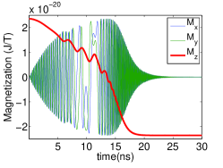
(a)

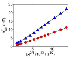
(b)

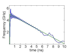
(c)

Figure 2: Color online. (a) Evolution of the three components of the magnetic moment $\mathbf{M}$ for a rotating field $B_{AC}^{rot}$. (b) Threshold amplitudes for a rotating field (red circles) and for an oscillating field with fixed direction (blue triangles) as a function of $|\alpha|^{3/4}$. (c) Instantaneous frequencies of the $M_{y}$ component of the magnetic moment (blue line) and of the applied rotating field $B_{AC}^{rot}$ (straight green line).

Figure 2a shows the evolution of each component of the magnetic moment $\mathbf{M}$ for a rotating field (for a field parallel to the $x$ axis the result is basically identical). For both cases, $M_{x}$ and $M_{y}$ oscillate in quadrature (this is the precession motion around the effective field $\mathbf{B}_{eff}$) while growing in amplitude, whereas $M_{z}$ drops from $+\mu_{S}$ down to $-\mu_{S}$. The magnetization switching occurs on a typical timescale of about 20 ns.

According to the theory fajans01 , the autoresonant mechanism is activated only if the amplitude of the excitation is above a threshold $b_{AC}^{th}\propto|\alpha|^{3/4}$, which is proportional to the frequency chirp rate $\alpha$. At zero temperature, the transition to the autoresonant regime around the threshold is very sharp and this scaling law is nicely confirmed by the numerical simulations (Fig. 2b). We note that a microvawe field rotating in the plane perpendicular to the anisotropy axis is slightly more efficient (i.e., it has a lower threshold) than a field oscillating along a given axis. Figure 2c displays the instantaneous frequency of the microwave excitation (a straight line, since the frequency varies linearly with time) together with the instantaneous frequency of the precessing magnetic moment. Both frequencies stay closely locked together, in accordance with the autoresonant mechanism. The instantaneous frequency was computed with an algorithm based on the Hilbert transform goswami .

Assuming that the amplitude is larger than $b_{AC}^{th}$, the switching time is determined by the frequency sweeping rate $\alpha$. Once the magnetic moment is captured into autoresonance, its nonlinear precession frequency is locked to the instantaneous excitation frequency $f(t)=f_{0}+\alpha t$ (remember that $\alpha<0$). If we define the switching time $\tau$ as the time it takes for the moment to cross the energy barrier and knowing that the frequency vanishes at the top of the barrier , we find $\tau=-f_{0}/\alpha$. Therefore, if we want the moment to switch rapidly we need a large sweeping rate $\alpha$. However, increasing the value of $\alpha$ also increases the required microwave field (see Fig. 2b). Beyond a certain value of $\alpha$, one would lose the benefit of field reduction provided by the autoresonance mechanism.

Our switching times can be compared to other methods, such as ballistic magnetization reversal He ; Bazaliy , which relies on a DC magnetic field that is switched on and off very rapidly. Ballistic reversal can be achieved in sub-nanosecond times, but requires a much larger field ($>1\rm T$), and the pulse duration must be within a tight time window, although the latter can be broadened using a spin-polarized current when dealing with large magnetic objects Zhang .

In contrast, our approach is not dependent on any form of feedback control, nor a precise tailoring of the external magnetic field (static or oscillating) and, being based on a resonant phenomenon, requires only small magnetic fields. As mentioned above, the autoresonant reversal time could also be shortened by using a larger chirp rate, at the expense of a stronger applied AC field.

IV Temperature effects

So far, we have only considered the zero-temperature (deterministic) case. In this section, we study the influence of thermal effects on the magnetization reversal. In isolated single-domain magnetic nanoparticles, the magnetization reversal by thermal activation is well described by the Néel-Brown model neel ; brown . According to this model, the thermal fluctuations cause the magnetic moment to undergo a Brownian-like motion about the axis of easy magnetization, with a finite probability to flip back and forth from one equilibrium direction to the other. The Néel-Brown model is well validated experimentally – see wernsdorfer for the case of 25 nm cobalt nanoparticles, and respaud for smaller nanoparticles (1-2 nm).

However, the temperatures that we consider here ($T<20$ K) are not large enough to produce this flipping effect, so that for all cases that we study the magnetization is initially (almost) aligned with the $z$ axis. Nevertheless, even if they are not capable of reversing the magnetization by themselves, thermal effects still have an influence on the efficiency of the switching technique, as we shall see in the forthcoming paragraphs.

For an isolated single-domain particle, Brown brown proposed to include the thermal fluctuations by augmenting the external field with a fluctuating field $\tilde{\mathbf{b}}(t)$ with zero mean and autocorrelation function given by:

$$\langle\tilde{b}_{i}(t)\tilde{b}_{j}(t^{\prime})\rangle=\frac{2\lambda k_{B}T}{(1+\lambda^{2})\gamma\mu_{S}}\delta_{ij}\delta(t-t^{\prime}),$$ (2)

where $i,j$ denote the cartesian components $(x,y,z)$, $\delta_{ij}$ is the Kronecker symbol (meaning that the spatial components of the random field are uncorrelated), and $\delta(t-t^{\prime})$ is the Dirac delta function, implying that the autocorrelation time of $\tilde{\mathbf{b}}$ is much shorter than the response time of the system. The temperature is thus proportional to the autocorrelation function of the fluctuating field.

At finite temperature, the thermal fluctuations drive the magnetic moment away from the $z$ axis and bring it to a randomly distributed orientation $(\theta_{0},\phi_{0})$ before the autoresonant field is activated. The initial amplitudes $\theta_{0}$ will then be described by a Rayleigh distribution $f(\theta_{0})=\frac{\theta_{0}}{\sigma^{2}}\exp\left(-\frac{\theta_{0}^{2}}{2\sigma^{2}}\right)$ where $\sigma$ is the scale parameter of the distribution. This randomness in the initial distribution creates a finite width in the transition to the autoresonant regime, so that the threshold is no longer sharp as in the zero-temperature case. This behavior was already observed in celestial dynamics wyatt ; quillen and superconducting Josephson resonators naaman . Note that the thermal fluctuations are active all along the simulations, although their main effect is to randomize the magnetization direction before the autoresonant field has had time to act. During the autoresonant excitation the thermal effects are present, but their effect is negligible compared to the oscillating field, at least for the range of temperatures considered here ($T<20\rm K$).

This effect can be quantified by the capture probability $P(b_{AC})$, defined as the probability for a magnetic moment to switch under the action of an autoresonant field of amplitude $b_{AC}$ (Fig. 3a). Following the calculations detailed in Appendix A, one can write this probability as

$$P(b_{AC})=-\frac{1}{4}\operatorname{erf}\left(\frac{c_{0}-b_{AC}}{\sqrt{2}\kappa\sigma}\right)\left[\operatorname{erf}\left(\frac{c_{0}-b_{AC}}{\sqrt{2}\kappa\sigma}\right)+2\right]+\frac{3}{4},$$ (3)

where $c_{0}$ is the threshold amplitude for $\theta_{0}=0$, and $\kappa$ is a numerically determined constant. The finite-temperature transition is no longer sharp, but instead displays a certain width $\Delta b_{AC}$, which is mathematically defined as the inverse slope of $P(b_{AC})$ computed at the inflexion point of the curve. It is also possible to derive an analytical expression for the width $\Delta b_{AC}$ as a function of the temperature and the volume of the nanoparticle (see Appendix A for details). One obtains:

$$\Delta b_{AC}\propto\sqrt{\frac{k_{B}T}{V}}.$$ (4)

We note that this dependence is the same as the one obtained from the Néel-Brown model neel ; brown for the fluctuating magnetic field arising from the random motion of the magnetic moment under the effect of the temperature.

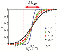
(a)

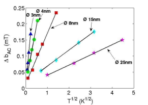
(b)

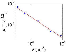
(c)

Figure 3: Color online. (a) Probability to capture the moment into autoresonance as a function of the microwave amplitude for a 25nm-diameter nanoparticle and different temperatures. Symbols: numerical simulations. Solid lines: theoretical results from Eq. (3). The transition width $\Delta b_{AC}$ is shown for the case with $T=10\rm K$. (b) Threshold transition width versus $T^{1/2}$ for various diameters. (c) Volume dependence of the parameter $A$ defined as $\Delta b_{AC}=AT^{1/2}$ . The straight line has a slope equal to $-1/2$.

The capture probability curves of Fig. 3a are fitted using the analytical expression of Eq. (3) (the fitting parameter is the product $\kappa\sigma$), with excellent agreement between the simulation data and the analytical estimate. Figure 3b shows that the transition width scales as the square root of the temperature, as predicted by Eq. (4), but the proportionality constant (i.e., the slope) depends on the volume of the nanoparticle. Plotting the slope as a function of the volume, it can be easily verified that $\Delta b_{AC}\propto V^{-1/2}$, thus confirming both scalings of Eq. (4). Therefore, increasing the size of the nanoparticle diminishes the effect of the temperature on the transition width, making the autoresonant switching observable at experimentally reachable temperatures.

The above results are of course limited by the applicability of the macrospin approximation, which will cease to be valid for large enough volumes. Nevertheless, for nanoparticles of size 15-30 nm (which covers the range considered in our study), Wernsdorfer and co-workers wernsdorfer found that the macrospin approximation is still acceptable. The validity of the macrospin approximation was also estimated in Ref. Gubin ; for cobalt nanoparticles, it is expected to break down for a diameter larger than roughly 32 nm (see Table 6.1 in Ref. Gubin ).

V Dipolar interactions

All the preceding results were obtained in the case of a single isolated nanoparticle. For an assembly of densely-packed nanoparticles, dipolar interactions may play a significant role, as was proven in recent numerical simulations kesserwan . The effect of dipole-dipole interactions on the relaxation time and, more generally, on the reversal process has been studied in several works, both theoretical Hansen ; Otero ; Dejardin and experimental Morup ; Dormann ; Farrell ; Hillion . Nevertheless, it is still a controversial issue, as opposite dynamical switching behaviors have been reported.

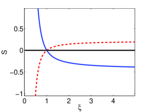
Figure 4: Color online. The $S(\xi)$ function for an assembly of nanoparticles with the easy axes oriented along the $\mathbf{e}_{z}$ direction (solid blue line) or normal to the $\mathbf{e}_{z}$ direction (dashed red line).

Here, we consider an assembly of interacting particles regularly distributed on a lattice with sites located at $\mathbf{r}=d_{1}(n_{1}\mathbf{e}_{x}+n_{2}\mathbf{e}_{y})+d_{2}(n_{3}\mathbf{e}_{z})$, where $d_{1}$ and $d_{2}$ are the centre-to-centre distances between particles in the $(\mathbf{e}_{x},\mathbf{e}_{y})$ plane and in the $\mathbf{e_{z}}$ direction, respectively, and $n_{1}$, $n_{2}$ and $n_{3}$ are integers not simultaneously equal to zero. The assembly is supplemented by a number of identical “replicas” in order to minimize the effect of the boundaries.

At the instant of capture, the moments are close to the $\mathbf{e}_{z}$ axis, and in the case of an $\mathbf{e}_{z}$-oriented assembly of nanoparticles, the dipolar field acting on each moment is also oriented along $\mathbf{e}_{z}$. In this configuration, the dipolar interactions can be taken into account via a self-consistent mean dipolar field denisov ; denisov1 $\mathbf{B}_{D}=8(\mu_{0}/4\pi)S(\xi)d_{1}^{-3}\overline{M}_{z}\mathbf{e}_{z}$ that acts on all the nanoparticles. Here, $\overline{M}_{z}$ is the $z$ component of the mean magnetic moment of the system and $S(\xi)$ is a structure function describing the geometry of the assembly, defined as:

$$S(\xi)=\frac{1}{8}\sum_{n_{1},n_{2},n_{3}}\frac{2\xi^{2}n_{3}^{2}-n_{1}^{2}-n_{2}^{2}}{(n_{1}^{2}+n_{2}^{2}+\xi^{2}n_{3}^{2})^{5/2}},$$ (5)

with $\xi\equiv d_{2}/d_{1}$. The sign of $S$ determines if the moments will order ferromagnetically ($S>0$, for essentially 1D systems where $\xi<1$) or antiferromagnetically ($S<0$, for 2D systems where $\xi>1$). The behavior of the function $S(\xi)$ is shown in Fig. 4 (solid blue line).

We studied two typical distributions of the nanoparticles: a 1D chain oriented along the $\mathbf{e_{z}}$ axis ($\xi\rightarrow 0,S\rightarrow\infty$), and a two dimensional configuration in the $(\mathbf{e}_{x},\mathbf{e}_{y})$ plane ($\xi\rightarrow\infty$, $S\rightarrow-1.129$). These configurations are represented schematically in Fig. 5. Intermediate values of $\xi$ correspond either to a set of stacked 2D arrays (when $\xi>1$), or a set of parallel 1D chains of nanoparticles (when $\xi<1$).

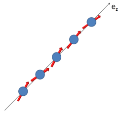
(a)

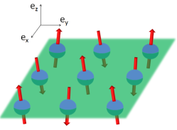
(b)

Figure 5: Color online. Schematic view of the nanoparticle configurations. (a) One-dimensional chain along the $\mathbf{e}_{z}$ axis: the particles are ordered ferromagnetically, with small tilts off the $\mathbf{e}_{z}$ axis due to the temperature. (b) Two-dimensional film in the $(\mathbf{e}_{x},\mathbf{e}_{y})$ plane with antiferromagnetic order.

It must be noted that the above considerations only apply to the cases where the easy axes are oriented along the $z$ directions, i.e., parallel to the chain in the 1D case, and normal to the plane in the 2D case. In other cases, the nature of the magnetic equilibrium may be different. For instance, a chain of particles with their easy axes oriented perpendicularly to the chain direction would behave antiferromagnetically; conversely, a 2D array of nanoparticles with the easy axes parallel to the plane of the array would display a ferromagnetic behavior at equilibrium. Indeed, for such cases, the function $S(\xi)$ displays an opposite behavior compared to the configurations of Fig. 5, namely it is negative for $\xi<1$ (1D antiferromagnetic) and positive for $\xi>1$ (2D ferromagnetic) (see Fig. 4, red dashed line).

Nevertheless, in our mean-field approach all the information about the geometry is included is the function $S(\xi)$. Different configurations that have the same value of $S$ behave identically in the mean-field limit. Therefore, in order to fix the ideas, in the remainder of this section we will focus on the geometries sketched in Fig. 5, which described by the solid blue curve on Fig. 4.

V.1 Two-dimensional planar configuration

The autoresonance mechanism is ineffective in a 2D configuration where the easy axes of the particles are oriented in the direction normal to the plane. The reason is that such a planar configuration naturally leads to an antiferromagnetic order, with half the moments pointing in the $+\mathbf{e}_{z}$ direction, and the other half in the $-\mathbf{e}_{z}$ direction. We have preformed a numerical simulation in order to illustrate this fact (see Fig. 6), using an assembly of nanoparticles with diameter equal to 25 nm and interparticle distances $d_{1}=50$ nm and $d_{2}\rightarrow\infty$.

We start, as usual, from a state where all moments are parallel to $+\mathbf{e}_{z}$, and then let the dipolar interactions create the anti-ferromagnetic order. Very quickly ($t\approx 5-10~{}\rm ns$), the dipolar interactions create an antiferromagnetic order: half of the moments reverse, while the other half stays parallel to $+\mathbf{e_{z}}$. We look at two representative moments: one that has switched to the $-\mathbf{e}_{z}$ direction (blue curve in Fig. 6) and one that has not (red curve).

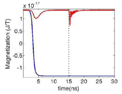
Figure 6: Color online. Magnetization dynamics in a planar assembly. Evolution of the $M_{z}$ component for a nanoparticle whose moment has reversed due to the dipolar interactions (blue) and for a nanoparticle whose moment stays aligned along $+\mathbf{e_{z}}$ (red curve). The oscillating field is switched on at $t=15$ ns (vertical dashed line).

At $t=15$ ns, once the magnetic order is settled, the rotating field is switched on and tries to capture and maintain the moments in autoresonance. The magnetic moment that had reversed to the $-\mathbf{e}_{z}$ direction (blue curve in Fig. 6) is maintained in that direction by the rotating autoresonant field, because this moment naturally precesses in the opposite way, so that the rotating field tends to counteract its precession. But the same rotating field is also unable to reverse a moment that points in the $+\mathbf{e}_{z}$ direction (red curve), because the interaction with its four nearest neighbours (all pointing along $-\mathbf{e}_{z}$) destroys the phase-locking even for $b_{AC}$ well above the threshold ($\approx 10b_{AC}^{th}$). This moment can be driven slightly away from its original $+\mathbf{e}_{z}$ axis (see the red curve at $t\approx 15-20$ ns), but soon the dipolar interactions become too strong and restore the antiferromagnetic order. The autoresonant technique is therefore inefficient for a planar assembly of magnetic nanoparticles.

V.2 One-dimensional linear chain

In contrast, a linear chain of nanoparticles with the easy axes oriented along the chain displays a ferromagnetic behavior, because $S>0$ for $\xi<1$ (see Fig. 4, solid blue line). At equilibrium, all the moments are oriented parallel to the $z$ direction, apart from small fluctuations due to the temperature (Fig. 5a). Therefore, there is a chance that the autoresonant mechanism may work in this type of configuration. In order to fix the ideas, we concentrate on a 1D chain of magnetic moments with fixed interparticle distance in the $(x,y)$ plane ($d_{1}=1\mu$m) and vary the distance $d_{2}$ along the $z$ axis from $1\mu$m to $26$nm, so that $\xi$ varies between 0.026 and 1.

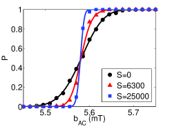
Figure 7: Color online. Capture probability as a function of the microwave amplitude for a chain of 25nm-diameter nanoparticles at $T=10$K, for different interparticle distances: $d_{2}=1\mu\rm m$ (black circles), $36\rm nm$ (red triangles), and $26\rm nm$ (blue squares). The corresponding values of $S(\xi)$ are indicated on the figure.

The effect of the dipolar interactions on the autoresonant switching is summarized in Fig. 7, which shows the capture probability as a function of the microwave amplitude for a 25nm-diameter nanoparticle at $T=10$K, for different interparticle distances along the $z$ axis. With decreasing interparticle distance (i.e., increasing dipolar interactions), the transition width shrinks, as was also observed for other physical systems barth . The dipolar interactions can almost completely erase the effect of the temperature for dense enough particle assemblies, as in the case with $d_{2}=26$nm in Fig. 7.

In reality, the self-consistent dipolar field does not stay aligned along $z$ during the reversal, so that the mean-field approximation fails at some point. However, its main effect occurs before the magnetic moment has reached the top of the barrier, and until then the approximation is valid. In other words, the dipolar interactions help the moments to be captured into autoresonance; once they are captured, the mean-field approximation is no longer accurate, but then the effect of the external field far outweighs that of the dipolar field, so that the error is irrelevant. Exact calculations for $N$ interacting moments (much more computationally demanding) also confirmed the above picture.

The dipolar interactions also slightly lengthen the switching time by increasing the effective potential barrier, which makes the resonant frequency $f_{r}$ higher. As we have to choose $f_{0}>f_{r}$, the switching time $\tau\sim f_{0}/\alpha$ also increases, but still remains of the order of 10-100 ns for all the cases studied.

VI Conclusions

We investigated the possibility to reverse the magnetization of a single-domain Co nanoparticle by combining a static field with a chirped microwave field. Using the LLG equation, we produced convincing evidence in favor of the autoresonance mechanism and showed that a chirped microwave field with a very small amplitude (a hundred times smaller than the static field) can efficiently reverse the magnetization.

Previous attempts barros to use a microwave field to reverse the magnetization showed that the microwave excitation should be modulated both in frequency and amplitude. Using the same parameters and configuration as in barros , but exploiting the autoresonance mechanism, we were able to reverse the magnetic moment with $b_{DC}=0.1$T and $b_{AC}=11$mT, reducing the amplitudes of both fields by roughly $30\%$. For an assembly of many nanoparticles, dipolar interactions can have a significant impact on the switching dynamics. The most favorable configuration is that of a linear chain of nanoparticles, for which the dipolar interactions can drastically reduce the effect of the temperature .

Compared to competing microwave techniques that use sophisticated feedback mechanisms, the autoresonance approach requires no fine tuning of the excitation parameters and thus appears to be a promising candidate for the fast control of the magnetization dynamics in densely-packed assemblies of magnetic nanoparticles.

Acknoledgments
We thank Dr. Jean-Yves Bigot for several helpful suggestions. We acknowledge the financial support of the French “Agence Nationale de la Recherche” through the project Equipex UNION, grant ANR-10-EQPX-52.

Appendix A Autoresonance transition with thermal noise

As discussed in more details in the article, the presence of noise broadens the transition to the autoresonant regime. In the main text, we mentioned that the transition width $\Delta b_{AC}$, Eq. 4, is proportional to $\sqrt{T/V}$, where $T$ is the temperature and $V$ is the volume of the nanoparticle. Here, we derive the full expression for $\Delta b_{AC}$.

The critical amplitude $b_{AC}^{th}$, beyond which the phase-locking is complete, is periodic in $\phi_{0}$ (the azimuthal angle at the onset of the oscillating field) and can therefore be expanded in a Fourier series barth :

$$b_{AC}^{th}=c_{0}+\kappa\theta_{0}\cos(\phi_{0}+\delta)+...$$ (6)

where the angles $(\theta_{0},\phi_{0})$ define the initial moment orientation, $c_{0}$ is the threshold amplitude for $\theta_{0}=0$, and $\kappa$ can be determined numerically. For small initial amplitudes, one can restrict the expansion to the lowest order in $\theta_{0}$. The capture probability (i.e., the probability to activate and maintain the autoresonant mechanism until magnetization reversal) can then be defined as

$$P(b_{AC})=\int_{0}^{\infty}P(\theta_{0},b_{AC})f(\theta_{0})d\theta_{0},$$ (7)

where $P(\theta_{0},b_{AC})=(1/\pi)\arccos[(c_{0}-b_{AC})/(\kappa\theta_{0})]$ and $f(\theta_{0})=\frac{\theta_{0}}{\sigma^{2}}\exp\left(-\frac{\theta_{0}^{2}}{2\sigma^{2}}\right)$ is the Rayleigh distribution characterizing the initial amplitudes resulting from the thermal noise. Actually it is more convenient to calculate

$$\frac{\partial P(b_{AC})}{\partial b_{AC}}=\int_{0}^{\infty}\frac{\partial}{\partial b_{AC}}(P(\theta_{0},b_{AC})f(\theta_{0}))d\theta_{0},$$ (8)

This calculation yields:

$$\frac{\partial P(b_{AC})}{\partial b_{AC}}=\frac{1}{\sqrt{2\pi}\kappa\sigma}e^{\frac{-(c_{0}-b_{AC})^{2}}{\sqrt{2}(\kappa\sigma)^{2}}}[1-\operatorname{erf}\left(\frac{-(c_{0}-b_{AC})}{\sqrt{2}\kappa\sigma}\right)],$$ (9)

Then, taking the antiderivative:

$$P(b_{AC})=-\frac{1}{4}\operatorname{erf}\left(\frac{c_{0}-b_{AC}}{\sqrt{2}\kappa\sigma}\right)\left[\operatorname{erf}\left(\frac{c_{0}-b_{AC}}{\sqrt{2}\kappa\sigma}\right)+2\right]+C,$$ (10)

Now, knowing that $\lim\limits_{b_{AC}\to\infty}P(b_{AC})=1$ we find the value of the integration constant $C=\frac{3}{4}$. Finally :

$$P(b_{AC})=-\frac{1}{4}\operatorname{erf}\left(\frac{c_{0}-b_{AC}}{\sqrt{2}\kappa\sigma}\right)\left[\operatorname{erf}\left(\frac{c_{0}-b_{AC}}{\sqrt{2}\kappa\sigma}\right)+2\right]+\frac{3}{4}.$$ (11)

The derivative of $P(b_{AC})$ gives a slope $P^{\prime}=(\sqrt{2\pi}\sigma\kappa)^{-1}$ at $b_{AC}=c_{0}$, whose inverse is defined as the transition width $\Delta b_{AC}$.

One can derive an analytical expression of the mean square displacement of the moment during a short time $\Delta t$ under the influence of the temperature, which is widely used in Monte Carlo simulations nowak ; chubykalo ; lyberatos . One can write the linearized LLG equation for the normalized moment ${\bf m}$ in the form:

$$\frac{dm_{x}}{dt} = L_{xx}m_{x}+L_{xy}m_{y},$$ (12)

$$\frac{dm_{y}}{dt} = L_{yx}m_{x}+L_{yy}m_{y}.$$ (13)

with

$$L_{xx}=L_{yy} = -{\frac{\gamma\lambda}{(1+\lambda^{2})}}m_{z}B_{z,eff},$$ (14)

$$L_{xy}=L_{yx} = -{\frac{\gamma}{(1+\lambda^{2})}}B_{z,eff}.$$ (15)

Also, close to the local energy minimum $E_{0}$, one can write the energy $E=E_{0}+\Delta E$ where $\Delta E=\frac{1}{2}\sum_{i,j}C_{ij}m_{i}m_{j}$ is the energy increase due to the small fluctuations of $m_{x}$ and $m_{y}$. Because of the interactions between the different subsystems the energy matrix $C_{ij}$ is nondiagonal, but it is possible to perform a transformation to the normal coordinates of the system and write $C$ as a diagonal matrix $\tilde{C}$. One can then write:

$$\Delta E=\frac{1}{2}(\tilde{C}_{xx}m_{x}^{2}+\tilde{C}_{yy}m_{y}^{2})$$ (16)

with $\tilde{C}_{xx}=\tilde{C}_{yy}=\frac{\mu_{S}}{m_{z}}B_{z,eff}$. The correlation matrix of the random forces $\mu_{ij}$ can be defined from $\tilde{C}_{ij}$ and $L_{ij}$ as $\mu_{ij}=-k_{B}T\sum_{k}{(L_{ik}\tilde{C}_{kj}^{-1}+L_{jk}\tilde{C}_{ki}^{-1})}$. Supposing that $m_{z}^{2}\approx 1$, the calculation yields:

$$\mu_{xx}=\mu_{yy}=\frac{2k_{B}T\lambda\gamma}{(1+\lambda^{2})\mu_{S}}.$$ (17)

Finally, one finds the mean square displacement by integrating over a finite time interval $\Delta t$:

$$\langle m_{x}^{2}\rangle=\langle m_{y}^{2}\rangle=\mu_{xx}\Delta t=\frac{2k_{B}T\lambda\gamma}{(1+\lambda^{2})\mu_{S}}\Delta t.$$ (18)

On the other hand, the expectation value of $\theta_{0}$ computed from the distribution $f(\theta_{0})$ is $\langle\theta_{0}\rangle=\sigma\sqrt{\pi/2}$. As $\langle\theta_{0}\rangle=\arcsin\left(\sqrt{\langle m_{x,0}^{2}\rangle+\langle m_{y,0}^{2}\rangle}\right)$, one can write the transition width as a function of the different system parameters:

$$\Delta b_{AC}=\frac{1}{P^{\prime}}=4\kappa(\Delta t)\sqrt{\frac{k_{B}T\lambda\gamma}{(1+\lambda^{2})M_{S}V}~{}\Delta t},$$ (19)

where we have used the expansion $\arcsin(x)=x+o(x^{2})$, valid for small initial amplitudes, and $\mu_{S}=M_{S}V$.

Note that $\Delta b_{AC}$ depends on $\Delta t$ only in the transient regime. Once the initial amplitude distribution has reached the Rayleigh equilibrium, the numerically determined “constant” $\kappa(\Delta t)$ exactly balances the term $\sqrt{\Delta t}$, so that $\Delta b_{AC}$ does not depend on $\Delta t$ anymore.

References

- (1) D. Weller et al., IEEE Trans. Magn. 36, 10 (2000).
- (2) S. P. Gubin Magnetic Nanoparticles (Wiley-VCH, Weinheim, 2009).
- (3) B. Hillebrands and J. Fassbender, Nature (London) 418, 493(2002).
- (4) C.H. Back et al., Science 285, 864 (1999).
- (5) Th. Gerrits, H.A.M. van den Berg, J. Hohlfeld, L. Bär, and Th. Rasing, Nature 418, 509(2002).
- (6) H.W. Schumacher et al., Phys. Rev. Lett. 90, 017201 (2003).
- (7) T. Seki, K. Utsumiya, Y. Nozaki, H. Imamura, and K. Takanashi, Nature Comm. 4, 1726 (2013).
- (8) D. Weller and A. Moser, IEEE Trans. Magn. 35, 4423 (1999).
- (9) S. Sun, C.B. Murray, D. Weller, L. Folks, and A. Moser, Science 287, 1989 (2000).
- (10) Ching-Ray Chang and Jyh-Shinn Yang, Phys. Rev. B 54, 11957 (1996).
- (11) J. Miltat, G. Albuquerque, and A. Thiaville, in Spin Dynamics in Confined Magnetic Structures I, B. Hillebrands and K. Ounadjela (Eds.), Topics Appl. Phys. 83 1-34 (Springer, Heidelberg, 2002).
- (12) C. Thirion, W. Wernsdorfer, and D. Mailly, Nature Mater. 2, 524 (2003).
- (13) N. Barros, M. Rassam, H. Jirari, and H. Kachkachi, Phys. Rev. B 83, 144418 (2011).
- (14) M. d’Aquino, C. Serpico, G. Bertotti, I. D. Mayergoyz, and R. Bonin IEEE Trans. Magn. 45, 3950 (2009)
- (15) J. Fajans and L. Friedland, Am. J. Phys. 69, 1096 (2001).
- (16) F. Peinetti, W. Bertsche, J. Fajans, J. Wurtele, and L. Friedland, Phys. Plasmas 12, 062112 (2005).
- (17) G. Marcus, L. Friedland, and A. Zigler, Phys. Rev. A 69, 013407 (2004).
- (18) B. Meerson and L. Friedland, Phys. Rev. A 41, 5233 (1990).
- (19) W. K. Liu, B. Wu, and J. M. Yuan, Phys. Rev. Lett. 75, 1292 (1995).
- (20) J. Fajans, E. Gilson, and L. Friedland, Phys. Rev. Lett. 82, 4444 (1999).
- (21) J. Fajans, E. Gilson, and L. Friedland, Phys. Plasmas 6, 4497 (1999).
- (22) L. Friedland, Phys. Rev. E 59, 4106 (1999).
- (23) G. Manfredi and P.-A. Hervieux, Appl. Phys. Lett. 91, 061108 (2007).
- (24) L. Cai, D. A. Garanin, and E. M. Chudnovsky, Phys. Rev. B 87, 024418 (2013).
- (25) K. Rivkin and J.B. Ketterson, Appl. Phys. Lett. 89, 252507 (2006).
- (26) Z. Wang and M. Wu, J. Appl. Phys. 105, 093903 (2009).
- (27) M. A. Shamsutdinov, L. A. Kalyakin, and A. T. Kharisov, Technical Physics 55, 860–865 (2010).
- (28) L. A. Kalyakin, M. A. Shamsutdinov, R. N. Garifullin, and R. K. Salimov, Phys. Metals Metallurgy 104, 107 (2007).
- (29) C. Goswami and A. E. Hoefel, Signal Processing 84, 1423 (2004).
- (30) L. He and W.D. Doyle, J. Appl. Phys. 79, 6489 (1996).
- (31) Ya. B. Bazaliy, J. Appl. Phys. 110, 063920 (2011).
- (32) Guang-Fu Zhang, Guang-hua Guo, Xi-guang Wang, Yao-zhuang Nie, and Zhi-xiong Li, AIP Advances 2, 042127 (2012).
- (33) C. D. Stanciu, F. Hansteen, A.V. Kimel, A. Kirilyuk, A. Tsukamoto, A. Itoh, and Th. Rasing, Phys. Rev. Lett. 99, 047601 (2007).
- (34) M. Jamet, W. Wernsdorfer, C. Thirion, D. Mailly, V. Dupuis, P. Mélinon, and A. Pérez, Phys. Rev. Lett. 86, 4676 (2001).
- (35) L. Néel, Ann. Géophys. 5, 49 (1949).
- (36) W. F. Brown, Phys. Rev. 130, 16776 (1963).
- (37) W. Wernsdorfer et al. Phys. Rev. Lett. 78, 1791 (1997)
- (38) M. Respaud et al. Phys. Rev. B 57, 2925 (1998)
- (39) M. C. Wyatt, Astrophys. J. 598, 1321 (2003).
- (40) A. C. Quillen, Mon. Not. R. Astron. Soc. 365, 1367 (2006)
- (41) O. Naaman, J. Aumentado, L. Friedland, J. S. Wurtele, and I. Siddiqi, Phys. Rev. Lett. 101, 117005 (2008).
- (42) H. Kesserwan, G. Manfredi, J.-Y. Bigot, and P.-A. Hervieux, Phys. Rev. B 84, 172407 (2011).
- (43) M.F. Hansen and S. Morup, J Magn. Magn. Mat. 184, L262 (1998).
- (44) J. Garcia-Otero, M. Porto, J. Rivas, and A. Bunde, Phys. Rev. Lett. 84, 167 (2000).
- (45) P.-M. Déjardin, J. Appl. Phys. 110, 113921 (2011).
- (46) S. Mørup and E. Tronc, Phys. Rev. Lett. 72, 3278 (1994)
- (47) J. L. Dormann, L. Bessais, and D. Fiorani, J. Physics C: Solid State Phys. 21, 2015 (1988).
- (48) D. Farrell, Y. Cheng, Y. Ding, S. Yamamuro, C. Sanchez-Hanke, C.-C. Kao, and S. A. Majetich, J. Magn. Magn. Mater. 282, 1 (2004).
- (49) A. Hillion, et al., IEEE Transactions on Magnetics 47, 3154 (2011).
- (50) S. I. Denisov and K. N. Trohidou, Phys. Status Solidi A 189, 265 (2002).
- (51) I. Barth, L. Friedland, E. Sarid, and A. G. Shagalov, Phys. Rev. Lett. 103, 155001 (2009).
- (52) W. Ruemelin, SIAM J. Numer. Anal. 19, 604 (1982).
- (53) N. G. Van Kampen, Stochastic Processes in Physics and Chemistry (North-Holland, Amsterdam, 1981).
- (54) P. E. Kloeden and E. Platen, Numerical Solution of Stochastic Differential Equations (Springer, Berlin, 1995).
- (55) U. Nowak, R. W. Chantrell, and E. C. Kennedy, Phys. Rev. Lett. 84, 163 (2000).
- (56) O. Chubykalo, U. Nowak, R. Smirnov-Rueda, M. A. Wongsam, R. W. Chantrell, and J. M. Gonzalez, Phys. Rev. B 67, 064422 (2003).
- (57) A. Lyberatos, D. V. Berkov, and R. W. Chantrell, J. Phys. Condens. Matter 5, 8911 (1993).
- (58) S. I. Denisov, Phys. Solid State 41, 1672 (1999).