Lifetimes of Metal Nanowires with Broken Axial Symmetry

Abstract

We present a theoretical approach for understanding the stability of simple metal nanowires, in particular monovalent metals such as the alkalis and noble metals. Their cross sections are of order one nanometer so that small perturbations from external (usually thermal) noise can cause large geometrical deformations. The nanowire lifetime is defined as the time required for making a transition into a state with a different cross-sectional geometry. This can be a simple overall change in radius, or a change in the cross section shape, or both. We develop a stochastic field theoretical model to describe this noise-induced transition process, in which the initial and final states correspond to locally stable states on a potential surface derived by solving the Schrödinger equation for the electronic structure of the nanowire numerically. The numerical string method is implemented to determine the optimal transition path governing the lifetime. Using these results, we tabulate the lifetimes of sodium and gold nanowires for several different initial geometries.

I Introduction

Nanowires made of monovalent metals, such as sodium, copper, and gold, live at the boundary between classical and quantum mechanics and exhibit some of the behavior of each. They are therefore of great interest from both a fundamental physics perspective as well as for technological applications. Their cross-sectional dimensions can be as small as half a nanometer (though several nanometers is far more typical) and their lengths at most a few tens of nanometers. At these length scales, the stresses induced by surface tension exceed Young’s modulus, making the wires subject to deformation under plastic flow BS05 , and therefore subject to breakup due to the Rayleigh instability Plateau1873 ; Burki03 . This in fact has been observed for copper nanowires annealed between 400 and 600^∘C MBCNT04 , as well as for copper and silver nanowires Bid05 ; Karim06 .

However, electron-shell filling effects stabilize these wires for radii near certain discrete “magic radii” BS05 . These radii correspond to conductance “magic numbers” that agree with those measured in experiments YYR99 ; YYR00 ; UBZSG04 ; Urban04 ; UBSG06 . This quantum stabilization, however, is only against small surface oscillations that can lead to breakup via the Rayleigh instability; it does not take into account thermal noise that can induce large radial fluctuations that can lead to breakup.

A self-consistent approach to determining lifetimes BSS05 , which modeled thermal fluctuations through a stochastic Ginzburg-Landau classical field theory, obtained quantitative estimates of alkali nanowire lifetimes BSS04 ; BSS05 in good agreement with experimentally inferred values YYR99 ; YYR00 . The theory, however, is limited to wires with a cylindrical symmetry. Urban et al. UBZSG04 ; UBSG06 , using a stability analysis of metal nanowires subject to non-axisymmetric perturbations, showed that, at certain mean radii and aspect ratios, Jahn-Teller deformations breaking cylindrical symmetry can be energetically favorable, leading to an additional class of stable nanowires with non-axisymmetric cross sections.

The mathematical problem of determining nanowire lifetimes in this more general case requires solution of a stochastic set of coupled partial differential equations corresponding to a stochastic Ginzburg-Landau field theory with two coupled fields, one corresponding to variations in mean radius and the other to deviations from axial symmetry. In particular, we consider here quadrupolar deformations of the nanowire cross-section, which cost less surface energy than higher-multipole deformations, and were shown to be the most common stable deformations within linear stability analyses UBSG06 ; Mares07 . The general mathematical treatment of such problems was discussed in GS10 ; GS11 . Of particular interest was the discovery of a transition in activation behavior not only as wire length varies BSS05 , but also as bending coefficients for the two fields vary GS11 .

In this paper, we use these results and those of Urban et al. UBZSG04 ; UBSG06 to construct a more general theory of lifetimes of nanowires with both axisymmetric and nonaxisymmetric cross-sections, as functions of temperature, strain, and other thermodynamic variables.

II Overview of the nanowire stability problem

Historically, there have been a number of studies on nanowires focusing on aspects ranging from growth techniques to electronic, mechanical, thermal and optical properties. There are several major laboratory techniques for synthesizing nanowires: suspension, vapor-liquid-solid (VLS), solution-based growth, and so on. The materials used to fabricate nanowires also vary, including metals (e.g., Ni, Pt, Au), semiconductors (e.g., Si, InP, GaN, etc.), and insulators (e.g., SiO₂, TiO₂). Usually, the focus is on nanowires with cross sections of the order of hundreds of nanometers or even a few micrometers IS06 ; Astafiev12 ; Schmid11 . However, the type of nanowire under study here is much smaller—at most a few nanometers in radius Agrait03 . The nanowires we study are mainly prepared via the suspension technique in either vacuum or air, as opposed to wires fabricated on a substrate and adhering to a surface.

Metal nanowires of atomic cross section are typically prepared using either a scanning tunneling microscope (STM) or a mechanically-controllable break junction (MCBJ) Agrait03 . In both cases, the nanowires are essentially freely suspended three-dimensional wires. In the STM setup, a nanowire is obtained by pushing the sharp STM tip into a substrate and then carefully retracting it in a controlled way. The contact formed in this way is of atomic dimensions ARV93 . If the tip is moved further away, the contact thins down and eventually breaks. In the MCBJ method Ruiten92pc ; Ruiten92prl , the sample is fixed onto an insulating substrate and then bent by a piezoelectric drive controlled by an applied voltage. The sample is pulled apart until the wire breaks, after which it reforms by reversing the process. The displacement between the electrodes can be controlled with accuracy down to 100fm. Because this setup is more stable against external vibration than the STM method, it allows more precise experiments on individual contacts. In both methods, the cross sectional area of the nanowire is inferred from conductance measurements using the corrected Sharvin formula UBSG06

$$\frac{G_{s}}{G_{0}}=\frac{k_{F}^{2}{\mathcal{A}}}{4\pi}-\frac{k_{F}{\mathcal{P}}}{4\pi}+\frac{1}{6},$$ (1)

which gives an approximation $G_{s}$ to the quantized conductance of an ideal metal nanowire in terms of geometrical quantities such as the wire’s minimal cross-sectional area ${\mathcal{A}}$ and corresponding cross section perimeter ${\mathcal{P}}$. Here $G_{0}=\frac{2e^{2}}{h}$ is the quantum of conductance and $k_{F}$ is the Fermi wavevector of the material.

The formation and breakup process is repeated thousands of times to derive a statistical histogram for the conductance Oleson95 ; CGO97 ; YYR99 (and therefore cross-sectional areas). The experiments can be performed at either ambient or cryogenic temperatures. Very small contacts consisting of four gold atoms in a row have been formed by means of this technique OKT98 . Although this type of experiment does not measure lifetimes of nanowires directly, rough estimates can be inferred from the existence of a conductance peak (which is evidence of a more stable wire, see Ref. Mares07 ) by knowing parameters of the experiment’s dynamics, in particular the speed of elongation of the wire. Typically, the existence of a conductance peak in a MCBJ experiment YYR99 implies a nanowire lifetime greater than one millisecond.

Based on these criteria, there is ample experimental evidence that nanowires made from sodium, gold and aluminum are stable with lifetimes greater than or of order milliseconds Urban04 ; UBSG06 ; Mares07 .

From a theoretical point of view, the stability of metal nanowires can be explained by quantum-size effects, or electron-shell effects, that can overcome the classical Rayleigh instability Plateau1873 in very thin wires. While the Rayleigh instability makes thin wires unstable once their surface tension exceeds their yield strength Zhang03 , shell effects can stabilize wires with certain preferred cross sections. The nanowire is a quantum system where conduction electrons are confined within the surface of the wire, with a Fermi wavelength comparable to the cross section linear dimension. This leads to electron-shell filling KSBG99 ; SBB97 ; RDEU97 , which provides an oscillating potential with multiple minima as a function of the cross section size and shape. This potential is called the electron-shell potential and its derivation will be discussed in detail in Sec. III. Figure 1 shows this shell potential for wires with a quadrupolar cross section as a function of the wire’s Sharvin conductance $G_{s}$ (related to the cross section area through Eq. (1)) and parameter $\lambda_{2}$ which describes the cross-section’s deviation from a disk (with $\lambda_{2}=0$).

$V_{shell}$

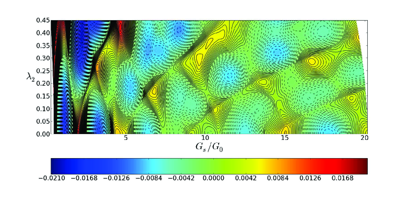
Figure 1: Contour plot of the electron-shell potential $V_{shell}$ as a function of the Sharvin conductance $G_{s}$ defined by Eq. (1) and the quadrupolar deformation parameter $\lambda_{2}$.

Quantum effects can thus stabilize the wire against breakup due to the Rayleigh instability. A linear stability analysis UBSG06 ; KSGG01 ; UG03 shows that cylindrical wires are most stable when the radius of the cross section takes a series of discrete values called the “magic radii”. It also finds that some wires with non-axisymmetric cross sections can be stabilized by electron-shell effects. In fact, comparison of the sequence of stable structures observed in experiments with linear stability analyses implies that some of the experimentally observed conductance peaks must correspond to wires with nonaxisymmetric cross sections Urban04 ; Mares07 .

However, linear stability analyses typically consider only stability towards small, long-wavelength deformations of the wire (see Refs. UG03 ; USG07 for a linear analysis including short-wavelength deformations). In particular, they do not consider changes of radius or breakup due to large fluctuations, which can be initiated by thermal noise, application of stress, or other destabilizing effects. Because the regions of stability are confined by finite energy barriers (as can be seen from Fig. 1), a given structure is at best metastable; its confining barriers can be surmounted by thermal (or other) noise.

The energy contours shown in Fig. 1 lead naturally to a description of the lifetime problem in which (meta)stable structures correspond to local energy minima; in the limit of low noise (thermal energy small compared to the lowest confining barrier), there is an optimal transition path along which the probability of a successful transition is maximized HTB90 . When the zero-noise dynamics are governed by a potential function (as is the case here), the “barrier” corresponds to a saddle point in the potential surface, that is, a fixed point whose linearized dynamics has a single unstable direction, all the others being stable. The transition rate is governed by Kramers’ formula

$$\mathit{\Gamma}\sim\Gamma_{0}\,\exp(-\Delta E/k_{B}T)$$ (2)

where $\Delta E$ is the difference in energy between the saddle and the initial state and $\Gamma_{0}$ is a prefactor depending on the fluctuations around each. In the low-noise limit, the lifetime of a metastable state is just the inverse of the Kramers’ transition rate. The problem then reduces to finding $\Delta E$ and $\Gamma_{0}$ as a function of the system parameters.

In the limit of weak noise, Wentzell and Freidlin (WF) VF showed that a rigorous asymptotic estimate for the rate of transition (i.e., probability of a successful transition per unit time) can be found by constructing an action functional, which gives the relative probabilities of different paths. It has been shown for gradient systems MS93a ; Marder96 that the optimal transition path is one in which the system climbs uphill against the gradient through a saddle state and then relaxes toward its final state.

Solving for the transition rate therefore requires knowledge of the saddle state. The model developed in GS10 allows for an analytical solution to the saddle state in the case of certain special potentials. To solve the nanowire stability problem, however, we need to find the transition path and lifetime in more general cases. The string method ERV02a ; ERenEric07 is a numerical scheme designed for this kind of problem. The procedure it uses is to first guess the optimal path and then let it evolve freely along the direction of steepest descent until equilibrium is reached. Details of the application of the string method to the kind of problem discussed here are given in GS11 .

In the case of cylindrical wires, the cross section of the wire can in principle shrink or grow under the influence of noise. However, nanowires studied in experiments are typically suspended between two electrodes that apply a strain on the wire that tends to pull it apart; as a consequence, transitions are biased toward smaller radii. In either case, the electrodes act as a “particle bath” that can supply or remove atoms from the wire.

The case of transitions between different radii under the assumption of constant axisymmetry was studied in BSS05 . This corresponds to transitions between energy minima along the $\lambda_{2}=0$ axis in Fig. 1, and the calculated lifetimes of cylindrical nanowires are comparable with experimental values. Here we include the effects of broken axial symmetry, so that transitions between any two minima in Fig. 1 can occur in principle.

The space of possible transitions is large. However, the study can be narrowed to those of greatest physical significance, guided by linear stability analyses UBZSG04 ; UBSG06 and experiments on alkali metal nanowires YYR99 ; YYR00 ; Urban04 . In particular, nanowires with electrical conductance $G/G_{0}=5,9$, and $29$, where $G_{0}=2e^{2}/h$ is the conductance quantum, were identified as the most stable nanowire structures with broken axial symmetry. We therefore concentrate on transitions from these local minima.

We will denote non-axisymmetric structures by $D$ (for deformed) and the cylindrical ones by $C$. So, for example, the non-axisymmetric structure with $G/G_{0}=5$ will be denoted $D5$, the cylindrical structure with $G/G_{0}=3$ will be denoted $C3$, and so on.

III The model

Metal nanowires have two main components which require different treatments: Conduction electrons have a wavelength at the Fermi surface that is of the order of the linear dimension of the wire cross section, and must therefore be treated quantum mechanically SBB97 , and positive ions which are much heavier and therefore have much shorter wavelengths. As a result, the ions can be treated classically Zhang03 and have a dynamics slow compared to that of the electrons, which can be treated separately Burki03 . This separation of timescales allows for a Born-Oppenheimer approximation where conduction electrons are considered at all times to be in equilibrium with the instantaneous ionic structure which confines them within the wire. Furthermore, for wires in the size regime dominated by electron-shell effects, the discrete atomic structure is unimportant and can be replaced by a continuum of positive charge (Jellium model Brack93 ; SBB97 ; Burki03 ): Electron shell effects are dominant over atomic shell effects in small wires (at least up to about $40\,G_{0}$ for alkali metal Urban04 and Al wires Mares07 , and are still present above that limit.)

These observations form the basis for the nanoscale free-electron model (NFEM SBB97 ; UBSG06 ; Urban10 ) which considers electrons in the wire to be free (other than being confined within the wire) and non-interacting. The former works best for s-shell metals, such as alkali and to some extent noble metals like gold, but has also been shown to perform well for metals whose Fermi surface in the extended zone scheme is nearly spherical, such as Al Mares07 . The limitation to non-interacting electrons has been shown to be a reasonable approximation for most metal nanowires KSG99 .

III.1 Energetics of the nanowire

The surface of a nanowire aligned along the $z$-axis can be described by a generalized radius function $R(z,\theta)$ in cylindrical coordinates, which can be written as a multipole expansion

$$R(z,\theta)=\rho(z)\left(\sqrt{1-\sum_{m}\lambda_{m}(z)^{2}/2}+\sum_{m}\lambda_{m}(z)\cos[m(\theta-\theta_{m}(z))]\right)\!,$$ (3)

where the sums run over the positive integers. $\rho(z)$ defines the mean radius at position $z$ along the wire, $\lambda_{m}(z)$ describes a multipolar deformation of order $m$, and $\theta_{m}(z)$ allows for a “twisting” of the wire cross section along $z$, which has no effect on the wire energy given the use of the adiabatic approximation (see below), and will therefore be dropped. The square root in Eq. (3) has been chosen so that the cross section area $\mathcal{A}=\pi\rho^{2}(z)$.

Urban et al. UBZSG04 ; UBSG06 have shown that, aside from axisymmetric wires, by far the most common stable nanowires are wires with a quadrupolar cross section ($m=2$). This is related to the fact that the surface-energy cost of deformations is proportional to $m^{2}$. Note that $m=1$ deformations correspond to a simple translation combined with higher-order deformations. For that reason, we will restrict ourselves to quadrupolar deformations with $m=2$, so that the shape of the wire will be described by two parameters: the mean radius $\rho(z)$ and the cross section deformation parameter $\lambda_{2}(z)$, which correspond to the shape shown in Fig. 2.

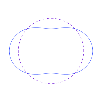
Figure 2: Cross section (solid line) of a nanowire with a quadrupolar deformation ($m=2$).

As long as the variation of the wire cross section along $z$ is slow enough (adiabatic approximation), any thermodynamic quantity can be written as an integral over $z$ of a local quantity that depends only on the cross section at $z$. This is in particular true SBB97 for the grand-canonical potential $\Omega_{e}$ of the conduction electrons, which is the appropriate thermodynamic potential for electrons in a wire connected to bulk electrodes (open system). $\Omega_{e}$ can thus be calculated for any wire of length $L$ as a functional of $\rho(z)$ and $\lambda_{2}(z)$

$$\Omega_{e}[T;\rho(z),\lambda_{2}(z)]=\int_{0}^{L}\!\text{d}z\,\omega(T,\rho(z),\lambda_{2}(z)),$$ (4)

where the local energy density $\omega(T,z)$ can be obtained numerically from the transverse energy levels $E_{n}(\rho(z),\lambda_{2}(z))$ using the WKB approximation. The energy levels themselves can be calculated numerically for any value of $\lambda_{2}$ and depend on $\rho$ in a simple way SBB97 ; UBSG06 .

On the other hand, any extensive thermodynamic quantity can be expressed in terms of a Weyl expansion Brack97

$$\mathit{\Omega}_{e}[\rho,\lambda_{2}]=-\omega\mathcal{V}+\sigma_{s}\mathcal{S}+\int_{0}^{L}V_{shell}[\rho,\lambda_{2}]\,dz,$$ (5)

where $\mathcal{V}$ and $\mathcal{S}$ are the wire’s volume and surface area, respectively. The last term is a quantum correction and can be taken as the definition of the electron shell potential $V_{shell}$, depicted in Fig. 1.

In the spirit of the Born-Oppenheimer approximation, the electronic grand canonical potential $\Omega_{e}$ is treated as the potential energy of the ions. Since the wire can also exchange ions with the bulk electrodes, the appropriate free energy determining the structure of the wire is the ionic grand canonical potential

$$\mathit{\Omega}_{a}[\rho,\lambda_{m}]=\Omega_{e}[\rho,\lambda_{m}]-\mu_{a}{\mathcal{N}}_{a}.$$ (6)

where $\mu_{a}$ is the chemical potential Burki03 ; BSS05 of the ions determined by the electrodes, and ${\mathcal{N}}_{a}$ is the number of ions in the wire.

III.2 Effective energy of deformations

While linear stability is a necessary condition for a nanostructure to be observed experimentally, it is not sufficient due to large stochastic deviations which can bring the wire out of its linearly stable state. Under the framework of the NFEM, we study the noise-induced fluctuations of the cross section by introducing two classical fields as perturbations to the parameters $\bar{\rho}$ and $\bar{\lambda}_{2}$ of the generalized radius function in Eq. (3):

$$\begin{aligned} \rho(z)&=\bar{\rho}\,\left(1+\phi_{1}(z)\right)\\ \lambda_{2}(z)&=\bar{\lambda}_{2}+\phi_{2}(z)\end{aligned}$$ (7)

where $(\bar{\rho},\bar{\lambda}_{2})$ is the location of the local minimum of the ionic grand canonical potential.

Expanding the ionic grand canonical potential (6) around $(\bar{\rho},\bar{\lambda}_{2})$ with respect to the fields $\phi_{1}$, $\phi_{2}$, and keeping terms up to quadratic order in the spatial derivatives, we get the fluctuation energy functional: The ionic grand canonical potential (6) becomes

$$\begin{aligned} \mathit{\Omega}_{a}[\rho,\lambda_{2}]&=\Omega_{a}[\bar{\rho}\,(1+\phi_{1}),\bar{\lambda}_{2}+\phi_{2}]\\ &=L\left\{\pi\sigma_{s}\bar{\rho}\,f[\bar{\lambda}_{2}]+\left(1-\frac{\bar{\rho}}{2}\partial_{\bar{\rho}}\right)V_{shell}[\bar{\rho},\bar{\lambda}_{2}]\right\}\\ &+\int_{-L/2}^{L/2}{\mathcal{H}}[\phi_{1}(z),\phi_{2}(z)]\,dz,\end{aligned}$$ (8)

where $2\pi\bar{\rho}f$ is the perimeter of the metastable nanowire’s cross section, and $f$ may be represented by a quartic polynomial with high accuracy:

$$f[\lambda_{2}]=1+\frac{3\lambda_{2}^{2}}{4}-\frac{9\lambda_{2}^{4}}{32}.$$ (9)

${\mathcal{H}}$ is the energy density of fluctuations at position $z$

$$\mathit{\mathcal{H}}[\phi_{1}(z),\phi_{2}(z)]=\\ \frac{1}{2}\pi\sigma_{s}\bar{\sigma}^{3}\left(\left\{2-\frac{\bar{\lambda}_{2}^{2}}{2}+\frac{71\bar{\lambda}_{2}^{4}}{16}\right\}(\phi_{1}^{{}^{\prime}})^{2}+2\bar{\lambda}_{2}\left\{1+\frac{\bar{\lambda}_{2}^{2}}{4}\right\}\phi_{1}^{{}^{\prime}}\phi_{2}^{{}^{\prime}}+\left\{1-\frac{5\bar{\lambda}_{2}^{2}}{4}\right\}(\phi_{2}^{{}^{\prime}})^{2}\right)\\ +U[\phi_{1}(z),\phi_{2}(z)]$$ (10)

with the effective potential

$$\begin{aligned} \mathit{U}[\phi_{1}(z),\phi_{2}(z)]&=-\bar{\rho}\,\partial_{\bar{\rho}}V_{shell}[\bar{\rho},\bar{\lambda}_{2}]\phi_{1}+2\pi\sigma_{s}\bar{\rho}\,f^{\prime}[\bar{\lambda}_{2}]\phi_{2}\\ &\quad-\bar{\rho}\left(\pi\sigma_{s}f[\bar{\lambda}_{2}]+\frac{1}{2}\partial_{\bar{\rho}}V_{shell}[\bar{\rho},\bar{\lambda}_{2}]\right)\phi_{1}^{2}\\ &+2\pi\sigma_{s}\bar{\rho}\,f^{\prime}[\bar{\lambda}_{2}]\phi_{1}\phi_{2}+\pi\sigma_{s}\bar{\rho}f^{\prime\prime}[\bar{\lambda}_{2}]\phi_{2}^{2}\\ &\quad+V_{shell}[\bar{\rho}(1+\phi_{1}),\bar{\lambda}_{2}+\phi_{2}]-V_{shell}[\bar{\rho},\bar{\lambda}_{2}].\end{aligned}$$ (11)

Here $\sigma_{s}$ is the material-dependent surface tension: for gold $\sigma_{s}=7.83\,(\mbox{eV}/\mbox{nm}^{2})$; for sodium $\sigma_{s}=1.39\,(\mbox{eV}/\mbox{nm}^{2})$. $L$ is the length of the wire. The electron shell potential $V_{shell}$ has to be obtained separately from solving for the electronic energy bands in the transverse direction numerically UBSG06 .

III.3 The dynamical system

As discussed in GS10 and GS11 , the time evolution of the fields under noise can be described by the coupled Langevin equations

$$\dot{\vec{\Phi}}=-\frac{\delta H[\vec{\Phi}]}{\delta\vec{\Phi}}+\sqrt{2\epsilon}\,\vec{\xi}(z,t)$$

where $\vec{\Phi}=\left(\begin{matrix}\phi_{1}\\ \phi_{2}\end{matrix}\right)$ and $\vec{\xi}(z,t)$ is Gaussian spatiotemporal white noise with $\epsilon=k_{B}T$. The saddle state is an extremum of the action $H[\vec{\Phi}]$ HTB90 and so the optimal transition path can be obtained numerically by evolving $\vec{\Phi}$ according to the noise-free form of the dynamical equations above.

For convenience, we make a change of variable $\phi_{1},\phi_{2}\to\psi_{1},\psi_{2}$ to eliminate the cross term $\phi_{1}^{\prime}\phi_{2}^{\prime}$ in Eq. (10). The two new fields are defined as:

$$\begin{aligned} \mathit{\psi}_{1}&=\phi_{1}+\frac{g_{12}}{g_{1}}\phi_{2}\\ \psi_{2}&=\phi_{2}\end{aligned}$$ (12)

with

$$\begin{aligned} g_{1}&=\pi\sigma_{s}\bar{\rho}^{3}(2-\frac{\bar{\lambda}_{2}^{2}}{2}+\frac{71\bar{\lambda}_{2}^{4}}{16})\\ g_{12}&=\pi\sigma_{s}\bar{\rho}^{3}\bar{\lambda}_{2}(1+\frac{\bar{\lambda}_{2}^{2}}{4})\\ g_{2}&=\pi\sigma_{s}\bar{\rho}^{3}(1-\frac{5\bar{\lambda}_{2}^{2}}{4})\,.\end{aligned}$$ (13)

The resulting equations of motion for $\psi_{1}$ and $\psi_{2}$ are

$$\dot{\psi}_{1} =g_{1}\psi_{1}^{{}^{\prime\prime}}+\bar{\rho}(\partial_{\bar{\rho}}V_{shell}[\bar{\rho},\bar{\lambda}_{2}])+2\bar{\rho}(\pi\sigma_{s}f[\bar{\lambda}_{2}]+\frac{1}{2}\partial_{\bar{\rho}}V_{shell}[\bar{\rho},\bar{\lambda}_{2}])\psi_{1}$$ (14)

$$\quad-(2\pi\sigma_{s}\bar{\rho}f^{\prime}[\bar{\lambda}_{2}]+2\bar{\rho}(\pi\sigma_{s}f[\bar{\lambda}_{2}]+\frac{1}{2}\partial_{\bar{\rho}}V_{shell}[\bar{\rho},\bar{\lambda}_{2}])\frac{g_{12}}{g_{1}})\psi_{2}$$

$$\quad-\bar{\rho}\,\partial_{\rho}V_{shell}[\rho,\lambda_{2}]$$

$$\dot{\psi}_{2} =(g_{2}-\frac{g_{12}^{2}}{g_{1}})\psi_{2}^{{}^{\prime\prime}}-(2\pi\sigma_{s}\bar{\rho}f^{\prime}[\bar{\lambda}_{2}]+\bar{\rho}\,\partial_{\bar{\rho}}V_{shell}[\bar{\rho},\bar{\lambda}_{2}]\frac{g_{12}}{g_{1}})$$

$$\quad+(2\bar{\rho}(\pi\sigma_{s}f[\bar{\lambda}_{2}]+\frac{1}{2}\partial_{\bar{\rho}}V_{shell}[\bar{\rho},\bar{\lambda}_{2}])\frac{g_{12}^{2}}{g_{1}^{2}}+\pi\sigma_{s}\bar{\rho}f^{\prime}[\bar{\lambda}_{2}]\frac{g_{12}}{g_{1}}-2\pi\sigma_{s}\bar{\rho}f^{{}^{\prime\prime}}[\bar{\lambda}_{2}])\psi_{2}$$

$$\quad-(2\pi\sigma_{s}\bar{\rho}f^{\prime}[\bar{\lambda}_{2}]+2\bar{\rho}(\pi\sigma_{s}f[\bar{\lambda}_{2}]+\frac{1}{2}\partial_{\bar{\rho}}V_{shell}[\bar{\rho},\bar{\lambda}_{2}])\frac{g_{12}}{g_{1}})\psi_{1}$$

$$\quad+\frac{g_{12}}{g_{1}}\bar{\rho}\,\partial_{\rho}V_{shell}[\rho,\lambda_{2}]-\partial_{\lambda_{2}}V_{shell}[\rho,\lambda_{2}]$$

where $\dot{\psi}=\partial\psi/\partial t$ and $\psi^{\prime}=\partial\psi/\partial z$. We now turn to the solution of the optimal transition path using the string method.

IV Results

In GS11 the string method was applied to the problem of noise-induced transitions in a two-component classical field theory. The transition path, or string, starts in a random configuration on the potential surface, with its two ends inside the basins of attraction of the initial and final states, respectively. The string is then allowed to evolve along the direction of the energy gradient, thereby determining the optimal transition path. The saddle state is the configuration of highest energy along this path. The results were consistent with the analytical solutions of GS10 , in particular, the transition of the saddle state from a homogeneous to an instanton configuration as $L$ increases beyond a critical value $L_{c}$.

In the following, we apply the same numerical scheme to the ionic grand canonical potential surface of a metal nanowire, in order to study lifetimes of wires whose cross sections correspond to the conductance plateaus $D5$ and $D9$.

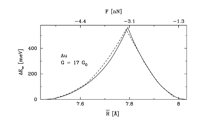
Figure 3: The activation barrier $\Delta E_{\infty}$ as a function of mean radius for the conductance plateau $G_{s}/G_{0}=17$ of gold. Solid curve: numerical result for the full potential; dashed curve: result from theoretical calculation BSS05 using the best cubic-polynomial fit to the full potential. The mean radius is related to the tensile stress (upper axis). This figure is taken from Ref. BSS05 .

It was found theoretically in BSS05 that both the activation barriers and the transition direction are sensitive to changes in stress of the order of 1nN. Fig. 3 shows the activation barrier for the transition of a cylindrical gold nanowire on the conductance plateau $G/G_{0}=17$ (denoted $C17$) to other linearly stable structures. To the left of the cusp, the transition proceeds in a direction corresponding to thinning (equivalently, moving to a lower conductance value); to the right, the transition proceeds via thickening (moving to a higher conductance value). The most stable structure of $C17$ corresponds to the maximum value of $\Delta E_{\infty}$, which is located at the cusp; at this point the activation barriers for thinning and growth are equal.

For a non-axisymmetric wire, by contrast, it is unlikely for thinning and growth processes to reach equilibrium at the same stress; the cusp in Fig. 3 is therefore absent. The greater richness of the configuration space for non-axisymmetric wires allows more options for escape from a given initial state; barriers are therefore generally lower (and lifetimes shorter) than in situations restricted to axial symmetry.

Detailed analysis shows that there are two types of instanton transition states that may arise as the initial state of the wire varies. The first corresponds to decay into the nearest cylindrical structure, and resembles an asymmetric hyperbolic tangent function with the longer arm coinciding with the initial configuration (see Fig. 4). The second corresponds to decay into (usually) the second-nearest neighbor cylindrical structure, and consists of multiple plateaus, each corresponding to a local minimum the transition goes through (see Fig. 5). We hereafter refer to the first as a “short instanton” and the second as a “long instanton.” The final state of the latter is farther from the initial state in configuration space than that of the former.

Switching between short and long instantons is caused by the change in the behavior of the activation barrier as a function of $L$. Within a given family of wires (e.g., $D5$) lying in a particular basin of attraction of the electron shell potential, there is a qualitative difference in the activation behavior of the thinner wires versus the thicker wires, which can be tuned by applying tensile/compressive stress. For thinner wires (e.g., under tensile stress), the energy of the short instanton first grows for $L<L_{c}$ and then reaches a plateau for $L>L_{c}$; for thicker wires (e.g., under compression), it continues growing as $L$ increases beyond $L_{c}$. The upper bound of the lifetime for the transition consequently grows without bound in the latter case as $L$ increases. Conversely, the energy of the long instanton approaches a finite asymptotic value as $L\to\infty$. Therefore, for thicker wires in a given family, the energies of the short and long instanton cross at a certain $L$, beyond which the short instanton transition state is no longer favorable (see Fig. 6).

The change in the energy behavior of the short instanton can be understood by modeling the transition using an asymmetric double well potential. In such a system (shown in Fig. 9a), the activation barrier of the state belonging to the upper well is finite and independent of $L$ as $L\to\infty$; consequently, the leading-order exponential term determining the lifetime [Eq. (2)] approaches a constant value. In the other direction, however, the lifetime of the lower well, as determined by its transition rate to the upper one (shown in Fig. 9b), is not bounded because the activation barrier grows with $L$: $\Delta E\sim C\cdot L$, with $C$ a constant determined by the energy difference between the two wells. When the cross section of the wire is varied by adjusting the applied tensile force, the two potential wells (representing the two linearly stable states) shift vertically relative to one another, until the lower well becomes the new upper well and vice-versa.

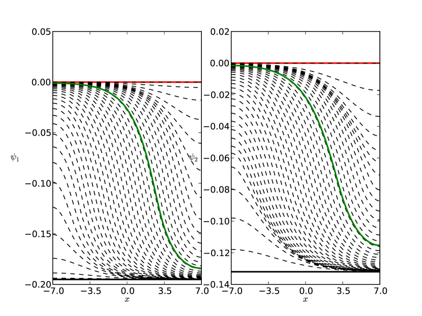
Figure 4: A typical configuration of the short instanton (green), where the transition starts from the initial $D5$ configuration at $G_{s}/G_{0}=5.55$ (red line) and ends at its nearest neighbor state $C3$ (thick black). Here a gold wire of length 1.2nm is considered. Dashed black lines are other intermediate states along the transition path.

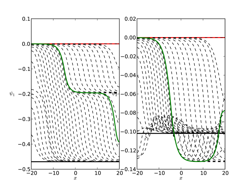
Figure 5: A typical configuration of the long instanton, where the transition starts from the initial $D5$ configuration at $G_{s}/G_{0}=5.56$ and ends at its second-nearest neighbor state $C1$. Note that there are two obvious plateaus in the shape of the long instanton, with one corresponding to the initial state and the other to the intermediate local minimum $C3$. Here a gold wire of length 3.3nm is considered. The line styles follow the same convention as in Fig. 4.

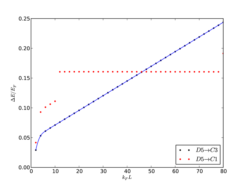
Figure 6: Activation barrier for thinning of the sodium $D5$ state, where the initial structure has $G_{s}/G_{0}=5.52$. There are two different final states: $C3$ and $C1$, to which the transition is via the short ($C3$) and long instanton ($C1$), respectively. The x-axis is in dimensionless units whose range corresponds to 0 to 8.8nm. Note that there is a discontinuity in the barrier of the transition $D5\to C1$, below which it suddenly drops and becomes inclined. For very short wires, the long instanton is not favorable and “collapses” into two short instantons, where the first is the saddle state of the transition $D5\to C3$ and the second is the saddle state of the transition $C3\to C1$. The string method can only select the saddle of the highest energy if there is more than one along the transition path; here it is that of $C3\to C1$, so that the activation barrier calculated increases with $L$.

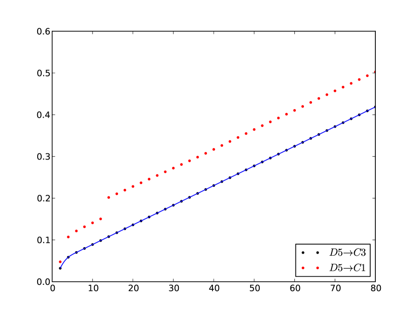
Figure 7: A typical situation at $G_{s}/G_{0}=5.56$ where the transition via long instanton turns unfavorable following that of the short instanton. The activation barrier of the long instanton (red dots) increases with $L$ as well as the lifetime so that the wire becomes more and more stable against thinning. The transition direction switches accordingly from thinning to growth.

Consider now the thinning process for wires under tension; as an example, we study the situation where the state $D5$ corresponds to the upper well and $C3$ to the lower well. Under tension, the activation barrier $\Delta E_{\infty}$, and hence the lifetime of the thinning process from $D5\to C3$, is always bounded. Under compression, however, $D5$ shifts downward to become the lower well and $C3$ the upper; now $\Delta E_{\infty}$ and the corresponding lifetime become unbounded as $L\to\infty$. The implication from this asymmetric double well model is that, to have a bounded lifetime, it is necessary to find a final state whose energy is lower than that of $D5$. $C1$ is such a state; the lifetime of $D5\to C1$ is bounded while that of $D5\to C3$ is not. These results are summarized in Fig. 9.

We can infer some of the dynamics of the process of escape from the shape of the long instanton. Fig. 5 implies that during the escape process part of the wire assumes the $C3$ state, which then bends further towards $C1$. We do not expect the long instanton to be a relevant intermediate state for escape from short wires as it would cost excessive bending energy in forming the necessary critical droplet. This conclusion is consistent with Fig. 6, in which the flat barrier of the long instanton disappears at small $L$.

As the wire is compressed and its cross section continues to grow, the energy of even $C1$ starts to shift upward and eventually it becomes the upper well relative to $D5$; the probability of thinning thereafter decreases (see Fig. 7). A similar analysis can be applied to $D9$, where the role of $C3$ is replaced by $D8$ and $C1$ by $C6$. The transition patterns of $D5$ and $D9$ are sketched in Fig. 8a and Fig. 8b.

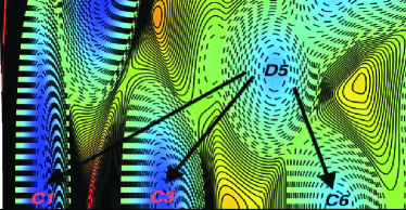
(a) Transition pattern of $D5$

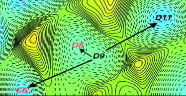
(b) Transition pattern of $D9$

Figure 8: Transition patterns for the structures $D5$ and $D9$. Both thinning and growth are drawn, where the final states of thinning are highlighted in red. Note that for growth only the nearest final state ($C6$ for $D5$ and $D11$ for $D9$) is shown for discussion purposes.

In Fig. 9, we denote the direction from the upper well to the lower one as the “forward” transition and the reverse as “backward”. With its activation barrier reaching a plateau as $L\to\infty$, the forward transition should occur more frequently than the backward one; we therefore refer to it as the transition direction. We emphasize that the terms “forward” and “backward” are defined relative to the upper well, that is, the higher-energy metastable state.

The switch from short-instanton to long-instanton
 
 

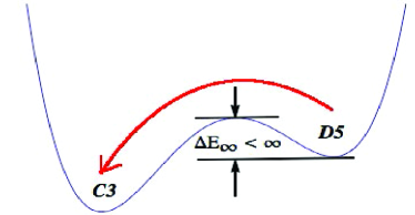
(a) Forward transition via short-instanton

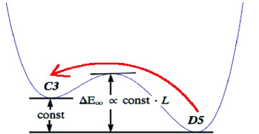
(b) Backward transition via short-instanton

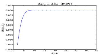
(c) Barrier of forward transition

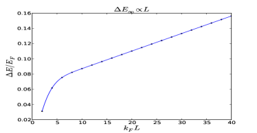
(d) Barrier of backward transition

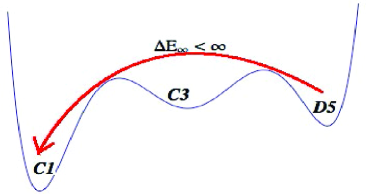
(e) The onset of long instanton

Figure 9: The first 4 subplots show the transition and the activation barrier of the $D5\to C3$ transition for Au via the short instanton. Two different situations are shown: under tension at $G_{s}/G_{0}=5.5$ (Fig. 9a, Fig. 9c) the activation behavior displays the characteristics of the forward transition, while under compression at $G_{s}/G_{0}=5.6$ (Fig. 9b, Fig. 9d) the activation behavior displays the characteristics of the backward transition. The activation barrier of the forward transition levels out as $L\to\infty$ while that of the backward transition grows almost linearly with $L$, following the discussion of the asymmetric double well model. The greater the difference in energy between the two metastable states, the faster $\Delta E$ grows with $L$. The last subplot sketches the transition from $D5$ to $C1$ via the long instanton, which sets a bound (as shown in Fig. (6)) on the barrier for thinning of $D5$ when the transition to $C3$ is backward.

In experiments, the wire is constantly subject to breakup and re-formation. Under elongation, the cross section typically samples all possible stable values before breakup. In reforming the nanowire, on the other hand, there is typically a jump to contact, and not all structures are clearly resolved in the conductance histogram. The relevant lifetime determining whether a given metastable structure is observed experimentally is therefore that governing the thinning process when the nanowire is under tension.

In the following sections, we calculate and display the lifetimes of the $D5$ and $D9$ structures for gold and sodium nanowires.

IV.1 Gold nanowires

In this subsection, we discuss our results for the stability of the $D5$ and $D9$ structures for gold nanowires.

For $D5$, $G_{s}/G_{0}=5.56$ corresponds to the critical cross section beyond which the long instanton plays a part in the determination of the lifetime. As the wire becomes thicker, the energy of the long instanton, and therefore the lifetime, increases monotonically. Eventually, the transition $D5\to C1$, occurring via the long instanton, becomes backward, essentially halting the thinning process. The evolution of the barrier for thinning is plotted in Fig. 10; the energy of the long instanton ranges up to $\Delta E_{\infty}=1000\,\mbox{meV}$, corresponding to a lifetime $\tau\approx 10^{7}\mbox{sec}$ at $T=300K$.

If one considers growth processes, the lifetime may be much shorter. The lifetime of the $D5\to C6$ process, for example, where $C6$ is a cylindrical state with a higher conductance value, is only of order $10^{-12}\mbox{sec}$. However, in experimental situations in which tensile stresses bias the system toward thinning, $D5$ should live long enough to be observed experimentally. Atoms can always leave the wire by diffusing out onto the surface of the bulk electrodes, while atoms incorporated into the bulk electrodes cannot readilly migrate into the wire, so that thickening may only be possible on reasonable timescales under compression.

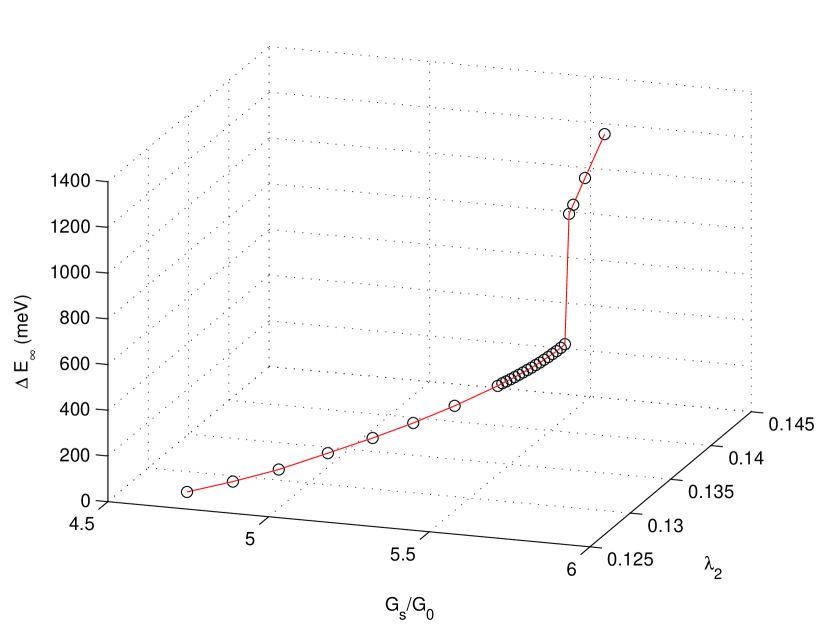
Figure 10: Activation barrier for thinning of the $D5$ structure in Au. The $G_{s}/G_{0}$ axis is related by the Sharvin formula to the continuous variation of the cross section resulting from the change of tensile force; the $\lambda_{2}$ axis is the corresponding variation in the degree of axial symmetry breaking. Below the critical cross section at $G_{s}/G_{0}=5.56$, the activation barrier $\Delta E_{\infty}$ is determined by the transition $D5\to C3$ via the short instanton, while for $G_{s}/G_{0}>5.56$ the activation barrier is determined by the transition $D5\to C1$ (long instanton). The curve stops at the point where the energy of the long instanton becomes unbounded and thinning thus surrenders to growth.

For the $D9$ structure, the analysis is similar to that for $D5$, except that the critical cross section for the onset of the long instanton is approximately $G_{s}/G_{0}=9.3$. Below this value, the likeliest transition is from $D9$ to $D8$ via the short instanton; above this value, the transition will be from $D9$ to $C6$ via the long instanton. For thicker wires, $D9$ could transition to $D11$ rapidly, with a lifetime of order a millisecond. Overall, $D9$ is quite stable against thinning, with a lifetime (determined by the long instanton) of $10^{3}\,\mbox{sec}$ at $T=100K$.

IV.2 Sodium nanowires

The qualitative features of the stability of sodium nanowires are similar to those of gold nanowires. However, lifetimes are significantly shorter (cf. Ref. BSS05 ) because of sodium’s smaller surface energy.

Nevertheless, $D5$ is quite stable against thinning, with a lifetime of $0.3\,\mbox{ms}$ at $T=100K$. The critical cross section above which the long instanton becomes relevant is $G_{s}/G_{0}=5.48$. $D9$ has a lifetime of $0.057\,\mbox{sec}$ at $T=60K$ or $0.00012\,\mbox{sec}$ at $T=80K$. The critical cross section for $D9$ is $G_{s}/G_{0}=9.3$. Both plateaus are unstable at room temperature and the same issues concerning growth vs. thinning apply to sodium as for gold.

V Discussion

The previous section discusses a mechanism — the interplay of transitions via short vs. long instantons — that is likely to play an important role in determining lifetimes of nonaxisymmetric wires. Physically, this interplay reflects the competition between classical and quantum effects (the latter encapsulated within the electron shell potential). In the classical regime, a long wire requires a large cross section to stabilize against the Rayleigh instability. However, when quantum effects are taken into account, the deep minima of the electron shell potential favor thinner structures, giving rise to “magic radii”. When quantum effects dominate, the thinning process is favored and the transition from thicker to thinner is forward; when classical effects dominate, the thinning transition becomes backward and hence less favorable. As the cross section is continuously varied from larger to smaller, we find that thinning is inhibited when the initial structure is thicker; the converse when it is thinner.

In the purely cylindrical case, thinning and growth reach equilibrium when the wire is at a particular cross-sectional area, as in Fig. 4 of Ref. BSS05 . The most stable structure and its lifetime can thus be defined at the cusp. In the non-axisymmetric case, however, there is no similar single point of equilibrium. The rate of growth is generally much faster than that of thinning, so that the wire may escape to a thicker state even if the lifetime for thinning is large. Experimentally, however, $D5$ and $D9$ are observable with lifetime of order milliseconds or larger. We believe this is due to the experimental situation in which applied stresses to the wire inhibit growth. Our model for both thinning and growth implicitly assumes that the transfer of atoms into and out of the wire is instantaneous. This assumption is a reasonable approximation for thinning but not for growth under normal experimental conditions. The observed stability of laboratory nanowires is largely restricted by thinning processes: in experiments the wire usually either thins or breaks up under the pulling force. Given this, our model is quite successful in predicting the stability of $D5$ and $D9$ conductance plateaus against thinning.

- (1) J. Bürki and C. A. Stafford, “On the stability and structural dynamics of metal nanowires,” Appl. Phys. A, vol. 81, p. 1519, 2005.
- (2) J. Plateau in Statique Expérimentale et Théorique des Liquides Soumis aux Seules Forces Molé culaires, Gautier-Villars, Paris, 1873.
- (3) J. Bürki, R. E. Goldstein, and C. A. Stafford, “Quantum necking in stressed metallic nanowires,” Phys. Rev. Lett., vol. 91, pp. 254501–1–254501–4, 2003.
- (4) M. E. T. Molares, A. G. Balogh, T. W. Cornelius, R. Neumann, and C. Trautmann, “Fragmentation of nanowires driven by Rayleigh instability,” Appl. Phys. Lett., vol. 85, pp. 5337–5339, 2004.
- (5) A. Bid, A. Bora, and A. K. Raychaudhuri, “Experimental study of rayleigh instability in metallic nanowires using resistance fluctuations measurements from 77k to 375k,” Proc. SPIE Int. Soc. Opt. Eng., vol. 5843, pp. 147–154, 2005.
- (6) S. Karim, M. E. Toimil-Molares, A. G. Balogh, W. Ensinger, T. W. Cornelius, E. U. Khan, and R. Neumann, “Morphological evolution of au nanowires controlled by rayleigh instability,” Nanotechnology, vol. 17, p. 5954, 2006.
- (7) A. I. Yanson, I. K. Yanson, and J. M. van Ruitenbeek, “Observation of shell structure in sodium nanowires,” Nature, vol. 400, pp. 144–146, 1999.
- (8) A. I. Yanson, I. K. Yanson, and J. M. van Ruitenbeek, “Supershell structure in alkali metal nanowires,” Phys. Rev. Lett., vol. 84, pp. 5832–5835, 2000.
- (9) D. F. Urban, J. Bürki, C.-H. Zhang, C. A. Stafford, and H. Grabert, “Jahn-Teller distortions and the supershell effect in metal nanowires,” Phys. Rev. Lett., vol. 93, pp. 186403–1–186403–4, 2004.
- (10) D. Urban, J. Bürki, A. Yanson, I. Yanson, C. Stafford, J. van Ruitenbeek, and H. Grabert, “Electronic shell effects and the stability of alkali nanowires,” Solid State Communications, vol. 131, p. 609, 2004.
- (11) D. F. Urban, J. Bürki, C. A. Stafford, and H. Grabert, “Stability and symmetry breaking in metal nanowires: The nanoscale free-electron model,” Phys. Rev. B, vol. 74, p. 245414, 2006.
- (12) J. Bürki, C. A. Stafford, and D. L. Stein, “Theory of metastability in simple metal nanowires,” Phys. Rev. Lett., vol. 95, pp. 090601–1–090601–4, 2005.
- (13) J. Bürki, C. A. Stafford, and D. L. Stein, “Fluctuational instabilities of alkali and noble metal nanowires,” in Noise in Complex Systems and Stochastic Dynamics II (Z. Gingl, J. M. Sancho, L. Schimansky-Geier, and J. Kertesz, eds.), pp. 367–379, Bellingham WA USA: SPIE Proceedings Series, 2004.
- (14) A. I. Mares, D. F. Urban, J. Bürki, H. Grabert, C. A. Stafford, and J. M. van Ruitenbeek, “Electronic and atomic shell structure in aluminium nanowires,” Nanotechnology, vol. 18, p. 265403, 2007.
- (15) L. Gong and D. L. Stein, “The escape problem in a classical field theory with two coupled fields,” J. Phys. A: Math. Theor., vol. 43, p. 405004, 2010.
- (16) L. Gong and D. L. Stein, “Noisy classical field theories with two coupled fields: Dependence of escape rates on relative field stiffness,” Phys. Rev. E, vol. 84, p. 031119, 2011.
- (17) S.-G. Ihn and J.-I. Song, “GaAs nanowires on si substrates grown by a solid source molecular beam epitaxy,” Appl. Phys. Lett., vol. 89, p. 053106, 2006.
- (18) O. V. A. et al., “Coherent quantum phase slip,” Nature, vol. 484, p. 355, 2012.
- (19) H. S. et al., “Fabrication of vertical inas-si heterojunction tunnel field effect transistors,” 69th Device Research Conference Digest, 2011.
- (20) N. Agraït, A. Levy Yeyati, and J. M. van Ruitenbeek, “Quantum properties of atomic-sized conductors,” Phys. Rep., vol. 377, pp. 81–380, 2003. and refs. therein.
- (21) N. Agraït, J. G. Rodrigo, and S. Vieira Phys. Rev. B, vol. 47, p. 12345, 1993.
- (22) C. J. Muller, J. M. van Ruitenbeek, and L. J. de Jongh Physica C, vol. 191, p. 485, 1992.
- (23) C. J. Muller, J. M. van Ruitenbeek, and L. J. de Jongh Phys. Rev. Lett., vol. 69, p. 140, 1992.
- (24) L. Olesen Phys. Rev. Lett., vol. 74, p. 2147, 1995.
- (25) J. L. Costa-Krämer, N. García, and H. Olin Phys. Rev. B, vol. 55, p. 12910, 1997.
- (26) H. Ohnishi, Y. Kondo, and K. Takayanagi, “Quantized conductance through individual rows of suspended gold atoms,” Nature, vol. 395, pp. 780–782, 1998.
- (27) C. H. Zhang, F. Kassubek, and C. A. Stafford, “Surface fluctuations and the stability of metal nanowires,” Phys. Rev. B, vol. 68, p. 165414, 2003.
- (28) F. Kassubek, C. A. Stafford, J. Bürki, and H. Grabert, “Universality in metallic nanocohesion: A quantum chaos approach,” Phys. Rev. Lett., vol. 83, pp. 4836–4839, 1999.
- (29) C. A. Stafford, D. Baeriswyl, and J. Bürki, “Jellium model of metallic nanocohesion,” Phys. Rev. Lett., vol. 79, pp. 2863–2866, 1997.
- (30) D. E. J. M. van Ruitenbeek, M. H. Devoret and C. Urbina, “Conductance quantization in metals: The influence of subband formation on the relative stability of specific contact diameters,” Phys. Rev. B, vol. 56, pp. 12566–12572, 1997.
- (31) F. Kassubek, C. A. Stafford, H. Grabert, and R. E. Goldstein, “Quantum suppression of the Rayleigh instability in nanowires,” Nonlinearity, vol. 14, pp. 167–177, 2001.
- (32) D. F. Urban and H. Grabert, “Interplay of Rayleigh and Peierls instabilities in metallic nanowires,” Phys. Rev. Lett., vol. 91, p. 256803, 2003.
- (33) D. F. Urban, C. A. Stafford, and H. Grabert, “Scaling theory of the peierls charge density wave in metal nanowires,” Phys. Rev. B, vol. 75, p. 205428, May 2007.
- (34) P. Hänggi, P. Talkner, and M. Borkovec, “Reaction-rate theory: Fifty years after Kramers,” Rev. Mod. Phys., vol. 62, pp. 251–341, 1990.
- (35) M. I. Freidlin and A. D. Wentzell, Random Perturbations of Dynamical Systems. New York/Berlin: Springer-Verlag, 1984.
- (36) R. S. Maier and D. L. Stein, “The escape problem for irreversible systems,” Phys. Rev. E, vol. 48, pp. 931–938, 1993.
- (37) M. Marder, “Statistical mechanics of cracks,” Phys. Rev. E, vol. 54, pp. 3442–3454, 1996.
- (38) W. E, W. Ren, and E. Vanden-Eijnden, “String method for the study of rare events,” Phys. Rev. B, vol. 66, pp. 052301–1–052301–4, 2002.
- (39) W. E, W. Ren, and E. Vanden-Eijnden, “Simplified and improved string method for computing the minimum energy paths in barrier-crossing events,” J. Chem. Phys., vol. 126, p. 164103, 2007.
- (40) M. Brack Rev. Mod. Phys., vol. 65, p. 677, 1993.
- (41) D. F. Urban, J. Bürki, C. A. Stafford, and H. Grabert, The Nanoscale Free-Electron Model, vol. 1. CRC Press, 2010.
- (42) F. Kassubek, C. A. Stafford, and H. Grabert, “Force, charge, and conductance of an ideal metallic nanowire,” Phys. Rev. B, vol. 59, p. 7560, 1999.
- (43) M. Brack and R. K. Bhaduri, Semiclassical Physics. Frontiers in Physics, Vol. 96, Addison-Wesley, 1997.