Probing sensitivity to charged scalars through partial differential widths: $\tau\rightarrow K\pi\pi\nu_{\tau}$ decays

Abstract

We define and test $\mathrm{CP}$-even and $\mathrm{CP}$-odd partial differential widths for the process $\tau\rightarrow K\pi\pi\nu_{\tau}$ assuming that an intermediate heavy charged scalar contributes to the decay amplitude. Adopting a model-independent approach, we use a Monte Carlo simulation in order to study the number of events needed to recover information on the new physics from these observables. Our analysis of the $\mathrm{CP}$-odd observables indicates that the magnitude of $f_{H}\eta_{P}$, which is related to the new-physics contribution, can be recovered with an uncertainty smaller than $3\%$ for $3\times 10^{6}$ events. This number of events would also allow one to retrieve certain parameters appearing in the SM amplitude at the percent level. In addition, we discuss the possibility of using the proposed observables to study specific models involving two Higgs doublets, such as the aligned two-Higgs-doublet model (A2HDM). This analysis is undertaken within the context of the upcoming Super B-factories, which are expected to provide a considerably larger number of events than that which was supplied by the B-factories. Moreover, a similar set of observables could be employed to study other decay modes such as $\tau\rightarrow\pi\pi\pi\nu_{\tau},\,\tau\rightarrow KK\pi\nu_{\tau}$ and $\tau\rightarrow KKK\nu_{\tau}$.

I Introduction

With the discovery of a new boson $H$ by the ATLAS Aad et al. (2012a) and CMS Chatrchyan et al. (2012a) collaborations, it is now very important to characterize this new particle in order to study the extent to which its features are in agreement with those predicted for the Higgs scalar within the Standard Model (SM). In particular, the spin of this new boson and its couplings to other particles have been carefully analyzed giving rise, with a high degree of confidence, to the conclusion that it has spin zero and that its couplings to the other particles are linearly correlated with their masses (see Refs. Ellis et al. (2014); Ellis and You (2013) and references therein). On the other hand, the possibility of an enlarged scalar spectrum is also being tested. In particular, from the high energy point of view, many searches for charged Higgs bosons decaying via $H\rightarrow\tau\nu_{\tau}$ have been performed by ATLAS and CMS (see, for example, Refs. Aad et al. (2012b)-Aaltonen et al. (2014)). These searches have found the data to be consistent with the expected SM background and have set limits on the branching ratio of top quark decays to a $b$ quark and a charged Higgs boson. The effects of the presence of a charged Higgs boson can also be studied indirectly by means of low energy observables defined, for example, for leptonic and semileptonic decays involving $B,D^{*},D,D_{s},K$ and $\pi$ mesons Beringer et al. (2012). Such decays have been widely studied at the B-factories by the Belle and BaBar collaborations. Moreover, the fact that no new particle has been observed at the present time may suggest that the new physics (NP) scale is out of reach for the LHC. Indirect searches for physics beyond the SM become particularly important within this context.

Among the various processes that can receive contributions from a charged Higgs boson, the $\tau$ lepton decays can be used to derive constraints on the scalar and pseudoscalar couplings of a charged scalar to fermions. The fact that $\mathrm{CP}$-violating effects are expected to be negligible within the SM means that a study of $\mathrm{CP}$-odd observables could reveal the presence of contributions from a charged Higgs boson, should the charged Higgs-fermion couplings violate $\mathrm{CP}$. Such an analysis has been carried out for the decay $\tau\rightarrow K\pi\pi\nu_{\tau}$ in Ref. Kiers et al. (2008), where the presence of a charged scalar contributing to the corresponding amplitude is assumed and two types of $\mathrm{CP}$-asymmetries are defined in addition to the usual partial rate asymmetry. In the present work, which extends the analysis of Ref. Kiers et al. (2008), we focus on the same decay $\tau\rightarrow K\pi\pi\nu_{\tau}$, with the main goal being to define and test various $\mathrm{CP}$-even and $\mathrm{CP}$-odd observables, on the one hand, and to study their sensitivity to a NP contribution due to the presence of a charged scalar, on the other. The decay under consideration, $\tau\rightarrow K\pi\pi\nu_{\tau}$, only involves a pseudoscalar coupling of a charged scalar to the up and strange quarks, in contrast to $\tau\rightarrow K\pi\nu_{\tau}$, for instance, which exclusively probes the scalar coupling D. M. Asner et al. (2000). It is also worth noting that the simplest $\tau$ decay with $\Delta S=1$ that probes the contribution arising from the exchange of a charged scalar is $\tau\rightarrow K\nu_{\tau}$. In fact, this decay involves exactly the same pseudoscalar coupling as $\tau\rightarrow K\pi\pi\nu_{\tau}$, and then imposes constraints on it.

For the analysis of the observables introduced below we use a large number of Monte Carlo simulated events. The size of the Monte Carlo sample has been chosen within the context of the upcoming Super B-factories, which are expected to significantly increase the luminosity as compared to the B-factories. The aim of this analysis is to provide insight into the number of events needed to extract information about the NP contribution as well as about the SM contributions, including the anomalous Wess-Zumino (WZ) term.

Although our primary focus in the present work is on a model-independent treatment of charged-scalar contributions to $\tau\rightarrow K\pi\pi\nu_{\tau}$, it is useful also to consider a specific scenario. Many models include one additional Higgs doublet, so that a charged Higgs is present. In particular, in the so-called aligned two-Higgs-doublet model (A2HDM), an alignment in flavour space of the Yukawa couplings of the two scalar doublets is enforced, leading to the elimination of flavour-changing neutral currents at tree level. This restrictive choice results in a highly predictive phenomenology for this model, which has been carefully explored (see Refs. Jung et al. (2010); Celis et al. (2013); Branco et al. (2012)). Of particular interest to us is not only the fact that the A2HDM includes potential new sources of $\mathrm{CP}$ violation but also that it imposes very restrictive constraints due to the three-family universality of the proportionality constants arising from the alignment in flavour space. The partial differential widths studied in this work can be considered as additional observables to test the A2HDM, specifically within the context of the Super B-factories, in which the possibility of extracting these distributions from the data is more plausible. In this paper we briefly discuss the usefulness of the proposed observables to probe the A2HDM.

The remainder of this paper is organized as follows. In Sec. II we write down the expression for the differential width for the decay $\tau^{-}\rightarrow K^{-}\pi^{-}\pi^{+}\nu_{\tau}$ in terms of the corresponding form factors, including both the NP and SM contributions. By integrating the differential width weighted by various angular functions, we define partial differential widths in Sec. III. Section IV introduces a set of $\mathrm{CP}$-even and $\mathrm{CP}$-odd observables derived from the weighted partial widths. The parameterization for the form factors, along with the set of reference values used later for the event simulation, are summarized in Sec. V. The analysis of the proposed $\mathrm{CP}$-even and $\mathrm{CP}$-odd observables is included in Sec. VI. Finally, in Sec. VII the decay is considered in the context of the A2HDM and in Sec. VIII some possibilities of testing the different assumptions used during the paper are briefly discussed. We summarize the main conclusions in Sec. IX. The Appendix contains some details relevant for the statistical analysis.

II Differential width for $\tau^{-}\rightarrow K^{-}\pi^{-}\pi^{+}\nu_{\tau}$

We start with the effective Hamiltonian that accounts for the decay $\tau^{-}\rightarrow K^{-}\pi^{-}\pi^{+}\nu_{\tau}$ within the SM

$$\mathcal{H}^{\mathrm{SM}}_{\mathrm{eff}}=\frac{G_{F}}{\sqrt{2}}\sin\theta_{c}\,[\bar{\nu}_{\tau}\gamma_{\mu}(1-\gamma_{5})\tau]\,[\bar{s}\gamma^{\mu}(1-\gamma_{5})u]+\mathrm{h.c.},\vspace*{3mm}$$ (1)

where $G_{F}$ is the Fermi constant and $\theta_{c}$ the Cabibbo angle. Possible NP effects due to a new charged scalar boson contributing to the decay may be included by adding the following terms to the effective Hamiltonian,

$$\mathcal{H}^{\mathrm{NP}}_{\mathrm{eff}}=\frac{G_{F}}{\sqrt{2}}\sin\theta_{c}[\eta_{S}\,\bar{\nu}_{\tau}(1+\gamma_{5})\tau\,\bar{s}u\,+\,\eta_{P}\,\bar{\nu}_{\tau}(1+\gamma_{5})\tau\,\bar{s}\gamma_{5}u]+\mathrm{h.c.},\vspace*{3mm}$$ (2)

where $\eta_{S}$ and $\eta_{P}$ are the scalar and pseudoscalar couplings, respectively. The hadronic matrix element $J^{\mu}\equiv\langle K^{-}(p_{1})\pi^{-}(p_{2})\pi^{+}(p_{3})|\bar{s}\gamma^{\mu}(1-\gamma_{5})u|0\rangle$ can be conveniently parameterized in terms of four form factors as follows,

$$J^{\mu}=\left[F_{1}(Q^{2},s_{1},s_{2})(p_{1}-p_{3})_{\nu}+F_{2}(Q^{2},s_{1},s_{2})(p_{2}-p_{3})_{\nu}\right]\!T^{\mu\nu}$$

$$+iF_{3}(Q^{2},s_{1},s_{2})\epsilon^{\mu\nu\rho\sigma}p_{1\nu}p_{2\rho}p_{3\sigma}+F_{4}(Q^{2},s_{1},s_{2})Q^{\mu},\vspace*{3mm}$$ (3)

where $Q^{\mu}=(p_{1}+p_{2}+p_{3})^{\mu}$, $T^{\mu\nu}=g^{\mu\nu}-Q^{\mu}Q^{\nu}/Q^{2}$, $s_{1}=(p_{2}+p_{3})^{2}$ and $s_{2}=(p_{1}+p_{3})^{2}$ and where we adopt the convention $\epsilon_{0123}=+1$, as in Refs. Kiers et al. (2008); Kuhn and Mirkes (1992). The functions $F_{1}-F_{4}$ are the form factors that arise from the different possible decay chains. $F_{1}$ and $F_{2}$ appear due to the decay chains involving the $K_{1}(1270)$ and $K_{1}(1400)$ resonances, $F_{3}$ is the anomalous Wess-Zumino term and $F_{4}$ is the scalar form factor, which is generally assumed to be negligible for this decay since there is no pseudoscalar resonance through which the decay can proceed Decker et al. (1994). The axial vector form factors $F_{1}$ and $F_{2}$ give the dominant contributions, while the anomalous vector form factor $F_{3}$ represents a subdominant contribution, as shown by numerical estimates D. M. Asner et al. (2000). The NP contribution coming from a scalar boson can be incorporated into the amplitude through the shift $F_{4}\rightarrow\tilde{F}_{4}=F_{4}+f_{H}\eta_{P}/m_{\tau}$ Kiers et al. (2008), where the pseudoscalar form factor $f_{H}$ is defined as

$$f_{H}=\langle K^{-}(p_{1})\pi^{-}(p_{2})\pi^{+}(p_{3})|\bar{s}\gamma_{5}u|0\rangle\,.\vspace*{3mm}$$ (4)

The starting point for our analysis will be the differential width for the decay obtained from Eq. (25) in Ref. Kiers et al. (2008) after integrating over the angle $\theta$. The angle $\theta$ is defined in the rest frame of the tau; it is the angle between the direction of the hadrons (“$\vec{Q}$”) in that frame and the direction of the tau in the laboratory frame. Performing the integration, we obtain

$$\frac{d\Gamma}{dQ^{2}ds_{1}ds_{2}d\gamma d\cos\beta}=\frac{A(Q^{2})}{4\pi}\Big{\{}\Big{[}\frac{2}{3}\langle K_{1}\rangle+\langle K_{2}\rangle+\frac{1}{3}\langle\overline{K}_{1}\rangle\big{(}3\cos^{2}\beta-1\big{)}/2\Big{]}\big{(}|B_{1}|^{2}+|B_{2}|^{2}\big{)}+$$

$$\hskip 73.97733pt+\Big{[}\frac{2}{3}\langle K_{1}\rangle+\langle K_{2}\rangle-\frac{2}{3}\langle\overline{K}_{1}\rangle\big{(}3\cos^{2}\beta-1\big{)}/2\Big{]}|B_{3}|^{2}+\langle K_{2}\rangle|B_{4}|^{2}$$

$$\hskip 102.43008pt-\frac{1}{2}\langle\overline{K}_{1}\rangle\sin^{2}\beta\cos 2\gamma\big{(}|B_{1}|^{2}-|B_{2}|^{2}\big{)}+\langle\overline{K}_{1}\rangle\sin^{2}\beta\sin 2\gamma\,\mathrm{Re}(B_{1}B^{*}_{2})$$

$$\hskip 56.9055pt+2\langle\overline{K}_{3}\rangle\sin\beta\sin\gamma\,\mathrm{Re}(B_{1}B^{*}_{3})+2\langle\overline{K}_{2}\rangle\sin\beta\cos\gamma\,\mathrm{Re}(B_{1}B^{*}_{4})$$

$$\hskip 56.9055pt+2\langle\overline{K}_{3}\rangle\sin\beta\cos\gamma\,\mathrm{Re}(B_{2}B^{*}_{3})-2\langle\overline{K}_{2}\rangle\sin\beta\sin\gamma\,\mathrm{Re}(B_{2}B^{*}_{4})$$

$$\hskip 34.14322pt+2\langle\overline{K}_{3}\rangle\cos\beta\,\mathrm{Im}(B_{1}B^{*}_{2})+\langle\overline{K}_{1}\rangle\sin 2\beta\cos\gamma\,\mathrm{Im}(B_{1}B^{*}_{3})$$

$$\hskip 39.83368pt-\langle\overline{K}_{1}\rangle\sin 2\beta\sin\gamma\,\mathrm{Im}(B_{2}B^{*}_{3})+2\langle\overline{K}_{2}\rangle\cos\beta\,\mathrm{Im}(B_{3}B^{*}_{4})\Big{\}}\,,$$ (5)

where

$$A(Q^{2})=\frac{G^{2}_{F}\sin^{2}\theta_{c}}{128(2\pi)^{5}}\frac{(m^{2}_{\tau}-Q^{2})^{2}}{m^{3}_{\tau}Q^{2}},$$ (6)

and

$$\langle K_{i}\rangle\equiv\frac{1}{2}\int^{\pi}_{0}K_{i}\sin\theta d\theta$$ (7)

(and similarly for $\langle\overline{K}_{i}\rangle$); the definitions of the $K_{i}$ and the $\overline{K}_{i}$ may be found in Ref. Kiers et al. (2008). As described in Ref. Kiers et al. (2008) (the definitions therein are identical to those in Ref. Kuhn and Mirkes (1992)), $\beta$ and $\gamma$ are Euler angles relating two coordinate systems used to specify the kinematics of the decay. Moreover, the functions $B_{1}-B_{4}$ are linearly related to the form factors as follows,

$$B_{1} = [F_{1}(p_{1}-p_{3})^{x}+F_{2}(p_{2}-p_{3})^{x}]$$ (8)

$$B_{2} = (F_{1}-F_{2})p^{y}_{1}$$ (9)

$$B_{3} = F_{3}\sqrt{Q^{2}}\,p^{y}_{1}p^{x}_{3}$$ (10)

$$B_{4} = \sqrt{Q^{2}}\left[F_{4}+\frac{f_{H}}{m_{\tau}}\eta_{P}\right].$$ (11)

Note that the form factors $F_{i}$ and $f_{H}$ are potential sources of strong phases, and that the only possible weak phase comes from the pseudoscalar coupling $\eta_{P}$. For future reference, let us also define the quantity $\overline{B}_{4}$, which is relevant for $\tau^{+}$ decays,

$$\overline{B}_{4}=\sqrt{Q^{2}}\left[F_{4}+\frac{f_{H}}{m_{\tau}}\eta^{*}_{P}\right].$$ (12)

In fact, the differential width for the $\mathrm{CP}$-conjugate decay $\tau^{+}\rightarrow K^{+}\pi^{+}\pi^{-}\bar{\nu}_{\tau}$ can be obtained by replacing $B_{4}$ by $\overline{B}_{4}$ in Eq. (5) since the only source of CP violation appears in $B_{4}$ through the coupling $\eta_{P}$. For further details of the quantities involved within this section see Ref. Kiers et al. (2008).

III Weighted Differential Widths

We now define observables that exploit the angular information that is available in the expression for the differential width. To do so, we employ weighting functions that allow us to isolate different contributions. Inspection of Eq. (5) reveals that it depends on nine different functions of the angles $\beta$ and $\gamma$. These functions form an orthogonal set; the functions, and their normalizations, are shown in Table 1.

Table 1: Angular weighting factors. The $h_{i}(\gamma,\beta)$ functions form an othogonal set. The normalization factors are given in the third column.

$i$	$\quad h_{i}(\gamma,\beta)$	$\iint[h_{i}(\gamma,\beta)]^{2}\sin\beta d\gamma d\beta$
$\,1\,$	$\quad 1$	$4\pi$
$\,2\,$	$\quad 3\cos^{2}\beta-1$	$16\pi/5$
$\,3\,$	$\quad\sin^{2}\beta\cos 2\gamma$	$16\pi/15$
$\,4\,$	$\quad\sin^{2}\beta\sin 2\gamma$	$16\pi/15$
$\,5\,$	$\quad\sin\beta\sin\gamma$	$4\pi/3$
$\,6\,$	$\quad\sin\beta\cos\gamma$	$4\pi/3$
$\,7\,$	$\quad\cos\beta$	$4\pi/3$
$\,8\,$	$\quad\sin 2\beta\cos\gamma$	$16\pi/15$
$\,9\,$	$\quad\sin 2\beta\sin\gamma$	$16\pi/15$

The orthogonality of the functions means that different terms in Eq. (5) can be easily isolated by performing angular integrations of the differential width weighted by these angular functions. Hence, we can define nine weighted differential widths,

$$\frac{d\Gamma_{i}}{dQ^{2}ds_{1}ds_{2}}\equiv\int\frac{d\Gamma}{dQ^{2}ds_{1}ds_{2}d\gamma\,d\cos\beta}h_{i}(\gamma,\beta)\sin\beta\,d\beta\,d\gamma,\quad\,i=1,...,9.$$ (13)

It is straightforward to perform the integrations in Eq. (13) using the information from Table 1. The results for the various weighted differential widths are shown in Table 2. The only weighted differential widths that include NP contributions are those with $i=1,5,6$ and $7$. Therefore, the remaining observables are clearly $\mathrm{CP}$-even.

Table 2: Weighted partial widths for the $\tau^{-}$ decay. The related expressions for the $\mathrm{CP}$-conjugate decay may be obtained by replacing $B_{4}$ by $\overline{B}_{4}$ everywhere it appears.

$i$	$(d\Gamma_{i}/dQ^{2}ds_{1}ds_{2})/A(Q^{2})$
1	$\left(\frac{2}{3}\langle K_{1}\rangle+\langle K_{2}\rangle\right)\left(|B_{1}|^{2}+|B_{2}|^{2}+|B_{3}|^{2}\right)+\langle K_{2}\rangle|B_{4}|^{2}$
2	$\frac{2}{15}\langle\overline{K}_{1}\rangle\left(|B_{1}|^{2}+|B_{2}|^{2}-2|B_{3}|^{2}\right)$
3	$-\frac{2}{15}\langle\overline{K}_{1}\rangle\left(|B_{1}|^{2}-|B_{2}|^{2}\right)$
4	$\frac{4}{15}\langle\overline{K}_{1}\rangle\,\mathrm{Re}(B_{1}B^{*}_{2})$
5	$\frac{2}{3}\langle\overline{K}_{3}\rangle\,\mathrm{Re}(B_{1}B^{*}_{3})-\frac{2}{3}\langle\overline{K}_{2}\rangle\,\mathrm{Re}(B_{2}B^{*}_{4})$
6	$\frac{2}{3}\langle\overline{K}_{3}\rangle\,\mathrm{Re}(B_{2}B^{*}_{3})+\frac{2}{3}\langle\overline{K}_{2}\rangle\,\mathrm{Re}(B_{1}B^{*}_{4})$
7	$\frac{2}{3}\langle\overline{K}_{3}\rangle\,\mathrm{Im}(B_{1}B^{*}_{2})+\frac{2}{3}\langle\overline{K}_{2}\rangle\,\mathrm{Im}(B_{3}B^{*}_{4})$
8	$\frac{4}{15}\langle\overline{K}_{1}\rangle\,\mathrm{Im}(B_{1}B^{*}_{3})$
9	$-\frac{4}{15}\langle\overline{K}_{1}\rangle\,\mathrm{Im}(B_{2}B^{*}_{3})$

IV Observables

Since we are assuming that $\mathrm{CP}$ is violated via the pseudoscalar coupling, the $\tau^{-}$ and $\tau^{+}$ distributions are not expected to be identical. There are in principle two ways to proceed. The first is to analyze the observables in Table 2 twice, once for the $\tau^{-}$ decay and once for the $\tau^{+}$ decay. Another possibility is to perform an analysis separately for the sum and the difference of the distributions. We will follow the latter approach, since it has the advantage that the difference between the $\tau^{-}$ and $\tau^{+}$ distributions is sensitive to the presence of $\mathrm{CP}$ violation. We define then the following distributions

$$\frac{d\Gamma^{\pm}_{i}}{dQ^{2}ds_{1}ds_{2}}\equiv\frac{1}{2}\left(\frac{d\Gamma_{i}}{dQ^{2}ds_{1}ds_{2}}\pm\frac{d\overline{\Gamma}_{i}}{dQ^{2}ds_{1}ds_{2}}\right),$$ (14)

where $d\overline{\Gamma}_{i}/dQ^{2}ds_{1}ds_{2}$ is obtained from $d\Gamma_{i}/dQ^{2}ds_{1}ds_{2}$ by the replacement $B_{4}\rightarrow\overline{B}_{4}$ (or, equivalently, $\eta_{P}\rightarrow\eta^{*}_{P}$); see Eqs. (11) and (12). We note that the quantities $d\Gamma^{+}_{i}/dQ^{2}ds_{1}ds_{2}$ and $d\Gamma^{-}_{i}/dQ^{2}ds_{1}ds_{2}$ are, by construction, $\mathrm{CP}$-even and $\mathrm{CP}$-odd, respectively. As was noted above, the only non vanishing $\mathrm{CP}$-odd distributions are those with $i=1,5,6$ and $7$, because the remaining weighted differential widths do not include NP contributions (i.e., they are independent of $B_{4}$).

Let us first consider the distributions with $i=1$. After projection onto $Q^{2},s_{1}$ or $s_{2}$, the $\mathrm{CP}$-even distribution with $i=1$ gives the $\mathrm{CP}$-average of the invariant mass distributions, which are the distributions that are usually studied in experimental analyses  D. M. Asner et al. (2000); Adachi et al. . The corresponding expression is obtained from Table 2,

$$\frac{d\Gamma^{+}_{1}}{dQ^{2}ds_{1}ds_{2}}=A(Q^{2})\left(\frac{2}{3}\langle K_{1}\rangle+\langle K_{2}\rangle\right)\left(|B_{1}|^{2}+|B_{2}|^{2}+|B_{3}|^{2}\right)+\frac{\langle K_{2}\rangle}{2}(|B_{4}|^{2}+|\overline{B}_{4}|^{2}).$$ (15)

The $\mathrm{CP}$-odd distribution with $i=1$ is given by

$$\vspace*{3mm}\frac{d\Gamma^{-}_{1}}{dQ^{2}ds_{1}ds_{2}}=A(Q^{2})\frac{\langle K_{2}\rangle}{2}(|B_{4}|^{2}-|\overline{B}_{4}|^{2})=2A(Q^{2})\langle K_{2}\rangle\frac{Q^{2}}{m_{\tau}}|F_{4}f_{H}\eta_{P}|\sin(\delta_{4}-\delta_{H})\sin(\phi_{H}),$$ (16)

where $\delta_{4}$ and $\delta_{H}$ denote the strong phases arising from the SM scalar form factor $F_{4}$ and the pseudoscalar form factor $f_{H}$, respectively, and $\phi_{H}$ is the weak phase present in $\eta_{P}$. The above expression is related to the well known partial rate asymmetry. As was noted in Ref. Kiers et al. (2008), the partial rate asymmetry is expected to be doubly suppressed due to the generally assumed smallness of $F_{4}$ and $\eta_{P}$. Expressions for the remaining non-zero $\mathrm{CP}$-even and $\mathrm{CP}$-odd weighted partial differential widths may be found in Table 3, where we have made use of the following definitions,

$$B^{(+)}_{4} \equiv \frac{1}{2}(B_{4}+\overline{B}_{4})=\sqrt{Q^{2}}\left[F_{4}+\frac{f_{H}}{m_{\tau}}\,\mathrm{Re}(\eta_{P})\right]$$ (17)

$$B^{(-)}_{4} \equiv \frac{1}{2}(B_{4}-\overline{B}_{4})=\frac{\sqrt{Q^{2}}\,if_{H}}{m_{\tau}}\,\mathrm{Im}(\eta_{P}).$$ (18)

Table 3: $\mathrm{CP}$-even (“$+$”) and $\mathrm{CP}$-odd (“$-$”) weighted partial widths. Several of the $\mathrm{CP}$-odd weighted partial widths are zero; these have been omitted.

$i(\pm)$	$(d\Gamma^{\pm}_{i}/dQ^{2}ds_{1}ds_{2})/A(Q^{2})$
$2(+)$	$\frac{2}{15}\langle\overline{K}_{1}\rangle\left(|B_{1}|^{2}+|B_{2}|^{2}-2|B_{3}|^{2}\right)$
$3(+)$	$-\frac{2}{15}\langle\overline{K}_{1}\rangle\left(|B_{1}|^{2}-|B_{2}|^{2}\right)$
$4(+)$	$\frac{4}{15}\langle\overline{K}_{1}\rangle\,\mathrm{Re}(B_{1}B^{*}_{2})$
$5(+)$	$\frac{2}{3}\langle\overline{K}_{3}\rangle\,\mathrm{Re}(B_{1}B^{*}_{3})-\frac{2}{3}\langle\overline{K}_{2}\rangle\,\mathrm{Re}\!\left(B^{*}_{2}B^{(+)}_{4}\right)$
$6(+)$	$\frac{2}{3}\langle\overline{K}_{3}\rangle\,\mathrm{Re}(B_{2}B^{*}_{3})+\frac{2}{3}\langle\overline{K}_{2}\rangle\,\mathrm{Re}\!\left(B^{*}_{1}B^{(+)}_{4}\right)$
$7(+)$	$\frac{2}{3}\langle\overline{K}_{3}\rangle\,\mathrm{Im}(B_{1}B^{*}_{2})-\frac{2}{3}\langle\overline{K}_{2}\rangle\,\mathrm{Im}\!\left(B^{*}_{3}B^{(+)}_{4}\right)$
$8(+)$	$\frac{4}{15}\langle\overline{K}_{1}\rangle\,\mathrm{Im}(B_{1}B^{*}_{3})$
$9(+)$	$-\frac{4}{15}\langle\overline{K}_{1}\rangle\,\mathrm{Im}(B_{2}B^{*}_{3})$
$5(-)$	$-\frac{2}{3}\langle\overline{K}_{2}\rangle\,\mathrm{Re}\!\left(B^{*}_{2}B^{(-)}_{4}\right)$
$6(-)$	$\frac{2}{3}\langle\overline{K}_{2}\rangle\,\mathrm{Re}\!\left(B^{*}_{1}B^{(-)}_{4}\right)$
$7(-)$	$-\frac{2}{3}\langle\overline{K}_{2}\rangle\,\mathrm{Im}\!\left(B^{*}_{3}B^{(-)}_{4}\right)$

Interestingly, from the definitions in Eqs. (17) and (18) and the results in Table 3, we note that it does not seem to be possible to extract $F_{4}$ (by itself) from the data when $\phi_{H}\neq\pm\pi/2$. In other words, there will always be an admixture of $f_{H}\eta^{R}_{P}$, and it will not be possible to distinguish them. However, if the coupling $\eta_{P}$ were purely imaginary, the factor $B^{(+)}_{4}$ would only depend on the scalar form factor $F_{4}$ and then the $\mathrm{CP}$-even observables with $i=5,6$ and $7$ would be useful for determining $F^{R,I}_{4}$.

In order to study the observables presented above (Table 3), we have made various assumptions that tend to simplify the analysis, in a manner similar to the approach that was followed in Ref. Kiers et al. (2008). First of all, note that the SM scalar form factor $F_{4}$ is generally assumed to be small for $\tau\rightarrow K\pi\pi\nu_{\tau}$, since there are no pseudoscalar resonances that mediate this decay. Therefore, we will neglect this contribution by setting $F_{4}=0$. Furthermore, we will assume that $f_{H}$ has a flat behaviour over the phase space (no $Q^{2},s_{1}$ and $s_{2}$ dependence) and does not contain strong phases. Thus, we set $f^{I}_{H}=0$. Under these assumptions the $1(-)$ distribution is reduced to zero, as can be seen from Eq. (16), while the $1(+)$ distribution becomes equal to the usual (unweighted) differential width, as follows from Eqs. (11), (12) and (15). Finally, in order to simplify and separate the analysis of the $\mathrm{CP}$-even and $\mathrm{CP}$-odd observables, we perform the analysis with $\phi_{H}=\pi/2$. For this particular value, $B^{(+)}_{4}=0$ and the NP contribution is removed from the $\mathrm{CP}$-even observables (see Eqs. (15) and (17), as well as Table 3). To set an input value for the quantity $|f_{H}\eta_{P}|$, we follow the approach adopted in Ref. Kiers et al. (2008), where it is assumed that the NP contribution to the width is hidden in the experimental uncertainty of the branching ratio. As shown there, the experimental uncertainty is saturated for $|f_{H}\eta_{P}|\simeq 17.9$. Thus, we take this value as a reference input. A few comments are in order at this point.

1. As is noted in Ref. Kiers et al. (2008), one way to obtain an estimate of the order of magnitude of $f_{H}$ is to compute $F_{4}$ within the context of Chiral Perturbation Theory (see Ref. Decker et al. (1994)) and then to relate $f_{H}$ to $F_{4}$ via the quark equations of motion. The latter step yields $f_{H}\sim Q^{2}F_{4}/m_{s}$. A numerical study along these lines, with kinematical variables sampled appropriately over the relevant phase space, shows that $\langle|f_{H}|\rangle\sim 14$, with $76\%$ of the values falling within the range $7$-$21\,$. Regarding the phase of $f_{H}$, one finds $\langle\arg\left(f_{H}\right)\rangle\simeq 0.97\,\pi$, so that $\left|\langle\mathrm{Im}(f_{H})\rangle\right|\ll\left|\langle\mathrm{Re}(f_{H})\rangle\right|$. Thus, it appears to be reasonable to assume that $f_{H}$ is real.

2. The NP parameter $|\eta_{P}|$ should scale as $m_{W}^{2}/M^{2}$ due to the charged scalar propagator, with $m_{W}$ and $M$ being the $W$ and charged scalar masses, respectively. If the charged scalar has electroweak couplings, it would be reasonable to assume that $\eta_{P}$ has a magnitude not exceeding unity.

3. Combining the estimates from the above two comments, we obtain $|f_{H}\eta_{P}|\sim 14$, which is similar to our reference value $|f_{H}\eta_{P}|=17.9$. As pointed out in Ref. Kiers et al. (2008), however, this estimate may well have large uncertainties due to the use of the quark equations of motion; a more realistic assumption would probably be to take $|f_{H}\eta_{P}|$ to be in the range $1$-$10$.

4. The decay channel $\tau^{-}\rightarrow K^{-}\nu_{\tau}$ also involves the pseudoscalar coupling $\eta_{P}$, so that this process can in principle be used to constrain the NP contribution to $\tau\rightarrow K\pi\pi\nu_{\tau}$. It turns out, however, that the constraints derived from $\tau^{-}\rightarrow K^{-}\nu_{\tau}$ are very sensitive to the values used for the strange quark mass and its uncertainty. By performing a crude estimate that takes into account the uncertainties of the $K^{-}$ decay constant, $f_{K^{-}}$, and makes use of the quark equations of motion, we obtain the constraint $|\eta^{I}_{P}|<0.364$ (recall our assumption that $\phi_{H}=\pi/2$). We note that this bound was derived by using the value $m_{s}=0.095\,\mathrm{GeV}$. On the other hand, if the quark mass is replaced by the meson mass, one finds $|\eta^{I}_{P}|<1.878$. By combining these constraints with the assumption that $1<|f_{H}|<10$, we obtain two different bounds, namely $|f_{H}\eta^{I}_{P}|<3.64$ and $|f_{H}\eta^{I}_{P}|<18.78$. Therefore, the constraints provided by the decay channel $\tau^{-}\rightarrow K^{-}\nu_{\tau}$ are not conclusive enough to discard our input value.

In much of the analysis that follows, we set $|f_{H}\eta_{P}|=17.9$. With the above comments in mind, however, we also include some results for $f_{H}\eta_{P}=1.79\,e^{i\pi/4}$ in Sec. VI.

V Parameterization of form factors

We now introduce the parameterization of the form factors $F_{1}-F_{3}$ appearing in the definitions of the quantities $B_{1}-B_{3}$ in the expression for the differential width (see Eqs. (5) and (8)-(10)). We write the form factors in terms of various Breit-Wigner functions in the following manner,

$$F_{1}(Q^{2},s_{1},s_{2}) = -\frac{2N}{3F_{\pi}}[C\cdot BW_{1270}(Q^{2})+D\cdot BW_{1400}(Q^{2})]\,BW_{K^{*}}(s_{2})$$ (19)

$$F_{2}(Q^{2},s_{1},s_{2}) = -\frac{N}{\sqrt{3}F_{\pi}}[A\cdot BW_{1270}(Q^{2})+B\cdot BW_{1400}(Q^{2})]\,T^{(1)}_{\rho}(s_{1})$$ (20)

$$F_{3}(Q^{2},s_{1},s_{2}) = \frac{N_{3}}{2\sqrt{2}\pi^{2}F^{3}_{\pi}}BW_{K^{*}}(Q^{2})\left[\frac{T^{(1)}_{\rho}(s_{1})+\alpha\,BW_{K^{*}}(s_{2})}{1+\alpha}\right].$$ (21)

The normalized Breit-Wigner propagators for the $K_{1}(1270)$ and the $K_{1}(1400)$ appearing in the axial vector form factors $F_{1}$ and $F_{2}$ are assumed to be D. M. Asner et al. (2000),

$$BW_{K_{1}}(Q^{2})=\frac{-m^{2}_{K_{1}}+im_{K_{1}}\Gamma_{K_{1}}}{Q^{2}-m^{2}_{K_{1}}+im_{K_{1}}\Gamma_{K_{1}}},$$ (22)

where $m_{K_{1}}$ and $\Gamma_{K_{1}}$ denote the mass and width for the corresponding $K_{1}$ state. The Breit-Wigner propagators for the $K^{*}$ and $\rho$ are taken to have energy-dependent widths (see Refs. D. M. Asner et al. (2000); Decker et al. (1993)),

$$BW_{R}(s)=\frac{-m^{2}_{R}}{s-m^{2}_{R}+i\sqrt{s}\Gamma_{R}(s)},$$ (23)

with

$$\Gamma_{R}(s)=\Gamma_{R}\frac{m^{2}_{R}}{s}\left(\frac{p}{p_{R}}\right)^{3},$$ (24)

where

$$p = \frac{1}{2\sqrt{s}}\sqrt{[s-(m_{1}+m_{2})^{2}][s-(m_{1}-m_{2})^{2}]}$$ (25)

$$p_{R} = \frac{1}{2m_{R}}\sqrt{[m^{2}_{R}-(m_{1}+m_{2})^{2}][m^{2}_{R}-(m_{1}-m_{2})^{2}]}.$$ (26)

In the above expressions the decay of the resonance $R$ to two particles with masses $m_{1}$ and $m_{2}$ is assumed. For the $K^{*}$, a single resonance with an energy-dependent width is assumed while the expression for the $\rho$ includes two different resonances:

$$T^{(1)}_{\rho}(s_{1})=\frac{BW_{\rho}(s_{1})+\beta BW_{\rho\prime}(s_{1})}{1+\beta}.$$ (27)

To fix the reference values for the parameters $A-D$ in Eqs. (19) and (20) we follow Ref. D. M. Asner et al. (2000), where constraints arising from the tabulated branching fractions of the $K_{1}$ resonances are imposed. Regarding the parameters $N$ and $N_{3}$ that regulate the contributions coming from the axial and anomalous form factors, respectively, we apply the criteria proposed in Ref. Kiers et al. (2008), in which $5\%$ of the $\tau\rightarrow K\pi\pi\nu_{\tau}$ width is ascribed to the $F_{3}$ term and the remaining $95\%$ to the $F_{1}$ and $F_{2}$ terms. For this computation, we have used the value of the branching ratio $\mathcal{B}(\tau\rightarrow K\pi\pi\nu_{\tau})$ obtained in Aubert et al. (2008), which is the most precise one at present (see Refs. Adachi et al. ; Lee et al. (2010)). All the reference values related to the form factors $F_{1}-F_{3}$ used in our analysis are listed in Table 4b. Among them, those corresponding to the form factors $F_{1}$ and $F_{2}$ are based on Ref. D. M. Asner et al. (2000). We note that a more recent and precise value for the mass and the width of the $K_{1}(1270)$ resonance obtained in Ref. Guler et al. (2011) from a signal-region fit for the channel $B^{+}\rightarrow J/\psi K^{+}\pi^{+}\pi^{-}$ is still in agreement with the input value used here. For the form factor $F_{3}$ we follow Ref. Decker et al. (1994), whereas for the $\rho$ and $\rho^{\prime}$ resonances the input values are guided by Refs. Finkemeier and Mirkes (1996); Kuhn and Santamaria (1990).

Table 4: Input values for the parameters entering in the form factors $F_{1}-F_{3}$. The left table (a) lists the dimensionless parameters while the right table (b) shows the masses and widths of the various resonances, along with the pion decay constant ($F_{\pi}$).

Parameter	Value
$\alpha$	$-0.2$
$\beta$	$-0.145$
$A$	$0.944$
$B$	$0$
$C$	$0.195$
$D$	$0.266$
$N$	$1.4088$
$N_{3}$	$1.4696$

(a)

Parameter	Value
$F_{\pi}$	$93.3\,\mathrm{MeV}$
$m_{1270}$	$1.254\,\mathrm{GeV}$
$\Gamma_{1270}$	$0.26\,\mathrm{GeV}$
$m_{1400}$	$1.463\,\mathrm{GeV}$
$\Gamma_{1400}$	$0.30\,\mathrm{GeV}$
$m_{K^{*}}$	$0.892\,\mathrm{GeV}$
$\Gamma_{K^{*}}$	$0.050\,\mathrm{GeV}$
$m_{\rho}$	$0.773\,\mathrm{GeV}$
$\Gamma_{\rho}$	$0.145\,\mathrm{GeV}$
$m_{\rho\prime}$	$1.370\,\mathrm{GeV}$
$\Gamma_{\rho\prime}$	$0.510\,\mathrm{GeV}$

(b)

VI ANALYSIS

In order to study the proposed observables we have performed two different analyses. In the first we have tested the SM hypothesis. In this case there are no $\mathrm{CP}$-violating effects present in this decay and hence the $\mathrm{CP}$-odd observables in Table 3 are zero. In the second analysis, we have performed various fits of the distributions arising from all of the observables in Table 3. Both analyses have been implemented by using our own Monte Carlo (MC) generator to simulate several sets of events with different sizes. The main goal of these two analyses is to estimate the number of events needed to detect the presence of NP (in the case of the SM test) and to extract the NP coupling (in the case of the fit to the $\mathrm{CP}$-odd observables). Furthermore, the study of the $\mathrm{CP}$-even observables aims to extract information about the resonant structure of the decay and, in particular, of the anomalous Wess-Zumino contribution.

We have focused our analysis on a scenario in which the NP parameter is assumed to be hidden in the experimental uncertainty of the branching ratio. Hence, as mentioned above, we have set the input value for the NP contribution to be $17.9\,e^{i\pi/2}$. In order to test the usefulness of the proposed observables when the NP contribution is considerably reduced, we have also performed an analysis of the $\mathrm{CP}$-odd observables in the case where $f_{H}\eta_{P}=1.79\,e^{i\pi/4}$.

VI.1 Monte Carlo Simulation

In order to simulate the distribution in Eq. (5), we have constructed a Monte Carlo event generator by applying von Neumann’s acceptance-rejection technique. Once a set of events has been generated that is consistent with the differential decay width, the different observables can be obtained by using suitable estimators. By employing our own event generator we are able to include different contributions to the differential decay width and to choose their parameterization. Various sets of events have been generated for the decay $\tau^{-}\rightarrow K^{-}\pi^{+}\pi^{-}\nu_{\tau}$ and for its $\mathrm{CP}$-conjugate, $\tau^{+}\rightarrow K^{+}\pi^{+}\pi^{-}\bar{\nu}_{\tau}$. The maximum number of events was taken to be $3\times 10^{6}$ for the case in which the NP parameter $f_{H}\eta_{P}$ is equal to $17.9\,e^{i\pi/2}$ and $10^{6}$ for the case with $f_{H}\eta_{P}=1.79\,e^{i\pi/4}$. Although the total number of events in these simulations is beyond the scope of the B-factories, it can be regarded as realistic within the context of the upcoming Super B-factories, which are expected to increase the design luminosity by approximately two orders of magnitude. In fact, the design luminosity at SuperKEKB is $8\times 10^{35}\,\mathrm{cm}^{-2}\mathrm{s}^{-1}$ and an integrated luminosity of $50\,\,\mathrm{ab}^{-1}$ is expected Akai (2013). Guided by the analysis performed in Ref. Adachi et al. (which was based on data collected by the Belle detector at KEKB) and taking into account the expected integrated luminosity at SuperKEKB, we can estimate the expected number of $\tau^{-}\rightarrow K^{-}\pi^{-}\pi^{+}\nu_{\tau}$ events. A conservative estimate gives $\sim 5\times 10^{6}$, which is above the maximum number of events we have simulated for the present analysis, $3\times 10^{6}$.

As was noted in Sec. IV, the pseudoscalar form factor has been assumed to be real and the SM scalar contribution has been neglected; thus, we have taken $f^{I}_{H}=F_{4}=0$ as inputs for the MC simulation. The input values related to the form factors $F_{1}-F_{3}$ are listed in Table 4b. As a test of the consistency of our event generator, the usual differential width distributions have been extracted from a set of $1\times 10^{5}$ simulated events. As can be seen from Fig. 1, the simulated distributions are in agreement with those obtained experimentally by the CLEO collaboration in Ref. D. M. Asner et al. (2000) and also with the expected distributions based on numerical computations Kiers et al. (2008). In addition to the contributions involving the form factors $F_{1}$ and $F_{2}$, the subdominant contribution from the W-Z term and the possible NP contribution have been incorporated in the plots.

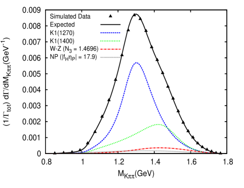
(a)

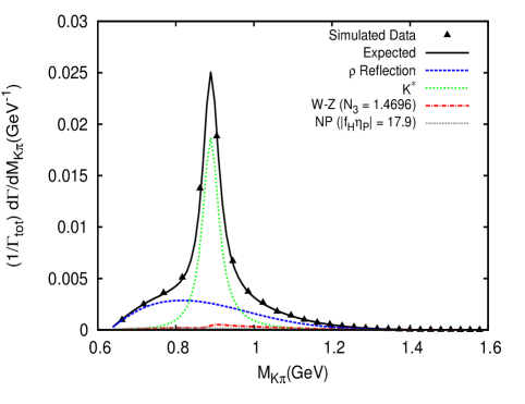
(b)

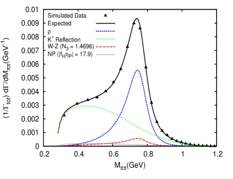
(c)

Figure 1: Plots of the differential widths $d\Gamma/dM$, including the different contributions from the decay chains along with the simulated data points obtained by using our MC generator. The $|f_{H}\eta_{P}|$ curve displays the NP contribution.

VI.2 SM Hypothesis test

The fact that the $\mathrm{CP}$-odd observables $5(-),6(-)$ and $7(-)$ are zero if the NP contribution is absent (i.e., if $f_{H}\eta_{P}=0$) allows for a test of the SM hypothesis by performing a Pearson’s $\chi^{2}$-test. To perform this test, we calculate $\chi^{2}$ for a particular observable $j(-)$ and then compute the quantity $P_{j}$, which is the probability that the hypothesis (the SM hypothesis in our case) would lead to a $\chi^{2}$ value greater than the one actually obtained,

$$\chi^{2}_{j}=\sum_{i=1}^{N_{\mathrm{bins}}}\left[\frac{d_{x}\Gamma^{-}_{j}(x_{i})}{\sigma^{(j)}_{i}}\right]^{2},\qquad P_{j}=\int_{\chi^{2}_{j}}^{\infty}f(z;n_{d})dz,\qquad j=5,6,7.$$ (28)

In the above expressions, $d_{x}\equiv d/dx$ with $x\equiv Q^{2},s_{1},s_{2}$, $N_{\mathrm{bins}}$ is the number of bins, $f(z;n_{d})$ is the $\chi^{2}$ distribution for $n_{d}$ degrees of freedom and $\sigma^{(j)}_{i}$ denotes the statistical uncertainty in the $i$-th bin for the observable $j(-)$ (see App. A). We remark that the values of the distributions in the numerator of the expression for $\chi^{2}_{j}$ given in Eq. (28) are extracted from the simulations. It is worth noting that this test is based on the assumption that the SM contribution only includes strong phases and therefore the only source of $\mathrm{CP}$-violation for the decay is a weak phase present in the NP contribution. Hence, the test itself does not depend on the particular value of the NP parameter, even when its robustness actually does (as we will show later). Tables 5 and 6 show results of the SM hypothesis test performed using the observables $d\Gamma^{-}_{5,6,7}/dx$, with different numbers of events, and taking $f_{H}\eta_{P}=17.9\,e^{i\pi/2}$.

Table 5: $P$-values corresponding to the observables $5(-)$ and $7(-)$. The number of events considered is given in the first column.

	$P$-$\mathrm{values}$
$N_{\mathrm{ev}}/100,000$	$d\Gamma^{-}_{5}/dQ^{2}$	$d\Gamma^{-}_{5}/ds_{1}$	$d\Gamma^{-}_{5}/ds_{2}$	$d\Gamma^{-}_{7}/dQ^{2}$	$d\Gamma^{-}_{7}/ds_{1}$	$d\Gamma^{-}_{7}/ds_{2}$
$5$	$0.933$	$0.754$	$0.175$	$0.0086$	$0.168$	$0.057$
$10$	$0.675$	$0.361$	$0.0018$	$0.00015$	$0.044$	$0.00013$
$15$	$0.198$	$0.062$	$0.000015$	$1.15\times 10^{-7}$	$0.00033$	$4.27\times 10^{-7}$
$20$	$0.286$	$0.055$	$2.73\times 10^{-7}$	$2.78\times 10^{-10}$	$8.14\times 10^{-6}$	$9.76\times 10^{-11}$

Table 6: $P$-values for the observable $6(-)$. The number of events is shown in the first column. Note that in this case fewer events were included in the simulations than were used in the previous table.

	$P$-$\mathrm{values}$
$N_{\mathrm{ev}}/100,000$	$d\Gamma^{-}_{6}/dQ^{2}$	$d\Gamma^{-}_{6}/ds_{1}$	$d\Gamma^{-}_{6}/ds_{2}$
$1$	$0.000024$	$0.0076$	$0.013$
$2$	$1.27\times 10^{-14}$	$1.05\times 10^{-7}$	$1.25\times 10^{-6}$
$3$	$<10^{-17}$	$6.66\times 10^{-16}$	$3.55\times 10^{-15}$
$4$	$<10^{-17}$	$<10^{-17}$	$<10^{-17}$

As shown in Table 6, the SM test for the observable $6(-)$ allows one to reject the SM hypothesis with as few as $10^{5}$ events. This is not the case for the other $\mathrm{CP}$-odd observables, which are not useful for rejecting the null hypothesis unless there are at least $5\times 10^{5}$ events. In fact, one can use this $\chi^{2}$ test to rank the various observables in terms of their sensitivity to the NP contribution. As is demonstrated by the data in Tables 5 and 6, the most sensitive observable appears to be the $Q^{2}$ projection of $6(-)$, which yields a $P$-value of $2.4\times 10^{-4}$ for $10^{5}$ events. Therefore, the $\mathrm{CP}$-odd differential width $6(-)$ (mainly its $Q^{2}$ projection) provides a suitable observable for rejecting the SM, since in the SM no $\mathrm{CP}$ violation effect is expected for this decay. In order to analyze the robustness of the test, we repeat the procedure with a sample of $10^{6}$ events for the scenario in which $f_{H}\eta_{P}=1.79\,e^{i\pi/4}$. In this case the test seems to loose its capability of rejection, even for the observable $6(-)$ (see Table 7). The tiny NP contribution in this case makes all three $\mathrm{CP}$-odd observables compatible with zero, at least for $10^{6}$ events. This reveals that a larger set of events ($>1\times 10^{6}$) is needed for these observables to be useful when the NP contribution is this small. However, this test can be regarded as an interesting possibility within the context of the upcoming Super B-factories, for which a conservative estimate of the expected number of events for the mode $\tau^{-}\rightarrow K^{-}\pi^{-}\pi^{+}\nu_{\tau}$ gives $\sim 5\times 10^{6}$, as was already mentioned in Sec. VI.1.

Table 7: $P$-values corresponding to the observable $6(-)$ for a NP contribution with $f_{H}\eta_{P}=1.79\,e^{i\pi/4}$.

	$P$-$\mathrm{values}$
$N_{\mathrm{ev}}/100,000$	$d\Gamma^{-}_{6}/dQ^{2}$	$d\Gamma^{-}_{6}/ds_{1}$	$d\Gamma^{-}_{6}/ds_{2}$
$10$	$0.53$	$0.93$	$0.99$

VI.3 Fitting Procedure

We have performed several fits of the one-dimensional distributions resulting from the projections of the observables listed in Table 3 onto $Q^{2}$, $s_{1}$ and $s_{2}$. Only the parameters appearing linearly in the expressions for the form factors $F_{1}$ and $F_{2}$, namely $A,B,C$, and $D$, along with the NP parameter, $f_{H}\eta_{P}$, have been taken into account as possible fit parameters, although we have also tested the possibility of recovering $N_{3}$ (which provides information regarding the Wess-Zumino contribution) from the fits. In order to construct the fitting function needed to apply the least squares method, we write each observable in terms of the parameters $\underline{\theta}=(A,B,C,D,N_{3},f_{H}\eta^{I}_{P})$ as follows,

$$\frac{d\Gamma^{\pm}_{i}}{dQ^{2}ds_{1}ds_{2}}=\sum_{j}f^{i(\pm)}_{j}(Q^{2},s_{1},s_{2})\zeta^{i(\pm)}_{j}(\underline{\theta}),$$ (29)

where the vectors $\zeta^{i(\pm)}$ depend on the parameters $\underline{\theta}$ and are listed in Table 8. By projecting Eq. (29) onto $x\equiv Q^{2},s_{1},$ or $s_{2}$, we obtain the corresponding expected value for the $i$-th projected partial differential width evaluated for the $k$-th bin of $x$:

$$\left(\frac{d\Gamma^{\pm}_{i}}{dx}\right)_{\mathrm{bin}\,\,k}=\sum_{j}c^{i(\pm)}_{kj}\zeta^{i(\pm)}_{j}(\underline{\theta}).$$ (30)

The matrices $c^{i(\pm)}$ in the above expression have dimension $N_{\mathrm{bins}}\times N^{i(\pm)}_{\mathrm{coeff}}$, with $N_{\mathrm{bins}}$ being the number of bins in the $x$ range and $N^{i(\pm)}_{\mathrm{coeff}}$ being the number of functions required to express the observable $i(\pm)$ in terms of the parameters $\underline{\theta}$ appearing in Eq. (29).

Table 8: List of the vectors $\zeta^{i(\pm)}$ appearing in Eq. (30) expressed in terms of the parameters in $\underline{\theta}$.

$i(\pm)$	$\zeta$
$2(+)$	$(C^{2},D^{2},CD,A^{2},B^{2},AB,AC,BC,AD,BD,N^{2}_{3})$
$3(+)$	$(C^{2},D^{2},CD,A^{2},B^{2},AB,AC,BC,AD,BD)$
$4(+)$	$(C^{2},D^{2},CD,A^{2},B^{2},AB,AC,BC,AD,BD)$
$5(+)$	$(N_{3}C,N_{3}D,N_{3}A,N_{3}B)$
$6(+)$	$(N_{3}C,N_{3}D,N_{3}A,N_{3}B)$
$7(+)$	$(CA,CB,DA,DB)$
$8(+)$	$(N_{3}C,N_{3}D,N_{3}A,N_{3}B)$
$9(+)$	$(N_{3}C,N_{3}D,N_{3}A,N_{3}B)$
$5(-)$	$(f_{H}\eta^{I}_{P}C,f_{H}\eta^{I}_{P}D,f_{H}\eta^{I}_{P}A,f_{H}\eta^{I}_{P}B)$
$6(-)$	$(f_{H}\eta^{I}_{P}C,f_{H}\eta^{I}_{P}D,f_{H}\eta^{I}_{P}A,f_{H}\eta^{I}_{P}B)$
$7(-)$	$(f_{H}\eta^{I}_{P}N_{3})$

The different matrices $c^{i(\pm)}$ are obtained by numerical integration of the appropriate function $f^{i(\pm)}_{j}(Q^{2},s_{1},s_{2})$. With the observables expressed as in Eq. (30), we proceed in general to minimize the quantity

$$\chi^{2}(\underline{\theta})=\sum_{j=1}^{N_{\mathrm{bins}}}\frac{(y^{\mathrm{sim}}_{j}-y^{\mathrm{exp}}_{j}(\underline{\theta}))^{2}}{\sigma^{2}_{j}},$$ (31)

where the $y^{\mathrm{sim}}_{j}$ are the values for a given observable extracted from the simulations, the $y^{\mathrm{exp}}_{j}$ are the corresponding expected values obtained by using the fitting function defined above, and the $\sigma_{j}$ are the statistical uncertainties associated with the simulation process (see App. A). We note that different choices of the parameters in $\underline{\theta}$ with respect to which $\chi^{2}(\underline{\theta})$ is minimized have been tested. The various resulting fits will be described in the following sections.

VI.4 Fit Results

We present now the results obtained by fitting the $\mathrm{CP}$-odd as well as the $\mathrm{CP}$-even observables (see Table 3). We consider these two sets of observables separately. In the case of the $\mathrm{CP}$-odd observables, we regard the NP parameter $f_{H}\eta_{P}$ as the unique free parameter and fix the remaining parameters to their input values. In the case of the $\mathrm{CP}$-even observables we focus on extracting information about the remaining parameters, $A,B,C,D$ and $N_{3}$, from our simulated data. This approach is facilitated by the assumptions mentioned in Sec.IV, namely that $F_{4}=f^{I}_{H}=0$ and $\phi_{H}=\pi/2$. Under these assumptions, the $\mathrm{CP}$-even observables in Table 3 do not depend on the NP contribution, and hence the input value for the parameter $f_{H}\eta_{P}$ is not involved in the analysis of these observables.

VI.4.1 $\mathrm{CP}$-odd observables

In order to recover the NP parameter $f_{H}\eta^{I}_{P}$ from the $\mathrm{CP}$-odd observables we perform a least squares fit by fixing the parameters $A,C$ and $D$ to their input values and setting the parameter $B$ to zero. The results obtained for two data sets (with different numbers of events) for the case $f_{H}\eta^{I}_{P}=17.9$ are displayed in Tables 9 and 10. The best fit value for $f_{H}\eta^{I}_{P}$ is more than $2.5\sigma$ away from zero for all of the $\mathrm{CP}$-odd observables, and is more compatible with the input value than with zero. Moreover, this is the case even when the number of events in the simulation is $5\times 10^{5}$. As was the case for the SM test proposed in the previous section, the observable $6(-)$ appears to be more precise than the other $\mathrm{CP}$-odd observables (judging by the smaller statistical uncertainty that it yields for the estimated parameter). As can be seen from the comparison between Tables 9 and 10, the statistical uncertainties are reduced by approximately $50\%$ when the number of events in the simulation is increased from $5\times 10^{5}$ to $3\times 10^{6}$.

Table 9: Best fit values for the parameter $f_{H}\eta^{I}_{P}$ obtained from the $\mathrm{CP}$-odd observables with a set of $5\times 10^{5}$ events. The input value for the NP parameter was set at $f_{H}\eta^{I}_{P}=17.9$. The difference between the best fit value and the input value, $|\Delta(f_{H}\eta^{I}_{P})|\equiv|\hat{f_{H}\eta^{I}_{P}}-f_{H}\eta^{I}_{P}|$, is included.

$N_{\mathrm{ev}}=5\times 10^{5}$
$d\Gamma^{-}_{i}/dQ^{2}$	$\hat{f_{H}\eta^{I}_{P}}$	$|\Delta(f_{H}\eta^{I}_{P})|$	$d\Gamma^{-}_{i}/ds_{1}$	$\hat{f_{H}\eta^{I}_{P}}$	$|\Delta(f_{H}\eta^{I}_{P})|$	$d\Gamma^{-}_{i}/ds_{2}$	$\hat{f_{H}\eta^{I}_{P}}$	$|\Delta(f_{H}\eta^{I}_{P})|$
$5$	$28\pm 11$	$0.9\sigma$	$5$	$21\pm 8$	$0.4\sigma$	$5$	$19\pm 5$	$0.2\sigma$
$6$	$17\pm 1$	$0.9\sigma$	$6$	$18\pm 1$	$0.1\sigma$	$6$	$17\pm 1$	$0.9\sigma$
$7$	$20\pm 4$	$0.5\sigma$	$7$	$17\pm 4$	$0.2\sigma$	$7$	$19\pm 4$	$0.3\sigma$

Table 10: Best fit values for the parameter $f_{H}\eta^{I}_{P}$ obtained from the $\mathrm{CP}$-odd observables with a set of $3\times 10^{6}$ simulated events . The difference $|\Delta(f_{H}\eta^{I}_{P})|\equiv|\hat{f_{H}\eta^{I}_{P}}-f_{H}\eta^{I}_{P}|$ is included.

$N_{\mathrm{ev}}=3\times 10^{6}$
$d\Gamma^{-}_{i}/dQ^{2}$	$\hat{f_{H}\eta^{I}_{P}}$	$|\Delta(f_{H}\eta^{I}_{P})|$	$d\Gamma^{-}_{i}/ds_{1}$	$\hat{f_{H}\eta^{I}_{P}}$	$|\Delta(f_{H}\eta^{I}_{P})|$	$d\Gamma^{-}_{i}/ds_{2}$	$\hat{f_{H}\eta^{I}_{P}}$	$|\Delta(f_{H}\eta^{I}_{P})|$
$5$	$18\pm 5$	$0.02\sigma$	$5$	$22\pm 3$	$1.4\sigma$	$5$	$18\pm 2$	$0.05\sigma$
$6$	$17.6\pm 0.4$	$0.8\sigma$	$6$	$18.0\pm 0.5$	$0.2\sigma$	$6$	$17.4\pm 0.5$	$1.0\sigma$
$7$	$17\pm 2$	$0.5\sigma$	$7$	$15\pm 2$	$1.5\sigma$	$7$	$17\pm 2$	$0.5\sigma$

We have also performed a least squares fit using the set of $10^{6}$ events with $f_{H}\eta_{P}=1.79\,e^{i\pi/4}$. In this case the best values obtained from the fit to the observables $5(-)$ and $7(-)$ become compatible with zero and have large statistical uncertainties, whereas the observable $6(-)$ is still the most precise one, giving best fit values that are more than $2\sigma$ away from zero and that recover the input value $f_{H}\eta^{I}_{P}=1.79\,\sin(\pi/4)\simeq 1.27$ even though the uncertainties are larger than those we obtain with $f_{H}\eta_{P}=17.9\,e^{i\pi/2}$ using a set of $10^{6}$ events. The results for the three projections of the observable $6(-)$ are shown in Table 11.

Table 11: Best fit values for the parameter $f_{H}\eta^{I}_{P}$ obtained from the observable $6(-)$ by using a set of $10^{6}$ simulated events with an input value $f_{H}\eta_{P}=1.79\,e^{i\pi/4}$ (so that $f_{H}\eta_{P}^{I}\simeq 1.27$).

$N_{\mathrm{ev}}=1\times 10^{6}$
$d\Gamma^{-}_{i}/dQ^{2}$	$\hat{f_{H}\eta^{I}_{P}}$	$|\Delta(f_{H}\eta^{I}_{P})|$	$d\Gamma^{-}_{i}/ds_{1}$	$\hat{f_{H}\eta^{I}_{P}}$	$|\Delta(f_{H}\eta^{I}_{P})|$	$d\Gamma^{-}_{i}/ds_{2}$	$\hat{f_{H}\eta^{I}_{P}}$	$|\Delta(f_{H}\eta^{I}_{P})|$
$6$	$1.9\pm 0.6$	$1.1\sigma$	$6$	$1.8\pm 0.8$	$0.7\sigma$	$6$	$1.7\pm 0.8$	$0.5\sigma$

Both the results obtained from the least squares fit and the SM test indicate the utility of using the observable $6(-)$ as a tool for investigating $\mathrm{CP}$-odd NP effects. On the one hand, the SM test shows this observable’s power to reject the SM hypothesis if there is actually a $\mathrm{CP}$-violating contribution; on the other hand, the least squares fit demonstrates how this observable can be used to recover the input value of the NP parameter. It is interesting to consider why the $6(-)$ observable is so much more sensitive to $\mathrm{CP}$ violation than are the other two $\mathrm{CP}$-odd observables that we have considered. This sensitivity arises from the dependence of the $\mathrm{CP}$-odd observables on the quantities $B_{i}$. As is evident in Table 3, the $7(-)$ observable is doubly suppressed due to the smallness of the W-Z and the NP contributions. Similarly, comparison of the $5(-)$ and $6(-)$ observables indicates that the latter exhibits a larger magnitude (and hence greater sensitivity to NP) because it depends on the quantity $B_{1}$, whereas the former depends on $B_{2}$; numerical study has shown that the magnitude of $B_{1}$ tends to be larger than that of $B_{2}$ within the allowed ranges of $Q^{2},s_{1}$ and $s_{2}$.

The above results are based on the assumption that $f_{H}$ has no $Q^{2},s_{1}$ or $s_{2}$ dependence. It is important to note, however, that a non-trivial dependence on the kinematical variables could appear due to the presence of final state interactions. The functional form of $f_{H}$ is unknown at present. Having said this, it is instructive to adopt a simple functional form for $f_{H}$ in order to test how the $6(-)$ distributions are modified. For the purpose of illustration, let us reconsider the expression for $f_{H}$ derived from the quark equations of motion, $f_{H}\sim(Q^{2}/m_{s})F_{4}$, where $F_{4}$ is assumed to be a constant. In order to set a reference value for $|F_{4}|$ the expression derived in Ref. Decker et al. (1994) within the context of Chiral Perturbation Theory has been used. A numerical analysis similar to that discussed in Sec. IV gives $\langle|F_{4}|\rangle\sim 0.54\,\mathrm{GeV}^{-1}$ and $\mathcal{O}(\langle\mathrm{Im}(F_{4})\rangle)<\mathcal{O}(\langle\mathrm{Re}(F_{4})\rangle)$. We set $F_{4}=0.54\,\mathrm{GeV}^{-1}$ and add a normalization factor in the expression for $f_{H}$, $\mathcal{N}$, so that the experimental uncertainty of the branching ratio is again saturated by the NP contribution. By taking $\phi_{H}=\pi/2$ we find the value $\mathcal{N}|\eta_{P}|=1.71$. Hence, $|f_{H}\eta_{P}|=\mathcal{N}(Q^{2}/m_{s})F_{4}|\eta_{P}|=1.71\times 0.54\,\mathrm{GeV}^{-1}(Q^{2}/m_{s})=0.92\,\mathrm{GeV}^{-1}(Q^{2}/m_{s})$. Figure 2 shows plots of the $6(-)$ distributions for the case $f_{H}\eta^{I}_{P}=17.9$ (blue solid line) along with the specific case presented above in which $f_{H}$ depends linearly on $Q^{2}$ (red dashed line).

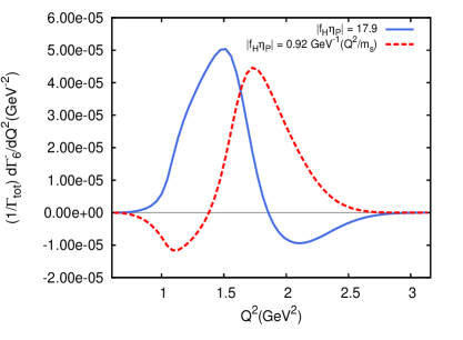
(a)

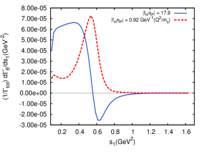
(b)

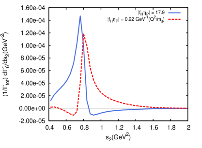
(c)

Figure 2: Plots of the distributions obtained from the observable $6(-)$ for $|f_{H}\eta_{P}|=17.9$ (blue solid line) and $|f_{H}\eta_{P}|=0.92\,\mathrm{GeV}^{-1}(Q^{2}/m_{s})$ (red dashed line). In the panels (a),(b) and (c) the projections onto $Q^{2},s_{1}$ and $s_{2}$ are displayed, respectively. The distributions are normalized to the total width of the $\tau$.

These distributions have been obtained numerically and normalized to the total width of the $\tau$ ($\Gamma_{\mathrm{tot}}$). As can be seen from the plots, the $6(-)$ distributions arising from the two approaches are comparable. On the one hand, the order of magnitude of each projection remains the same in both cases. On the other hand, the maxima of the distributions do not change significantly from one approach to the other. Based on these facts, it would be reasonable to expect that the number of events needed for recovering the NP parameter from the $6(-)$ distributions in the case $|f_{H}\eta_{P}|=17.9$ would also be enough for the case $|f_{H}\eta_{P}|\propto Q^{2}$. In this sense, the presence of a linear $Q^{2}$ dependence in $f_{H}$ should not spoil the sensitivity of the $6(-)$ distributions to the NP contribution with respect to the case in which $|f_{H}|$ is assumed to be a flat function. Hence, this specific case shows that the proposed observables could be useful even when there is a non-trivial dependence of $|f_{H}|$ on $Q^{2},s_{1}$ and $s_{2}$.

VI.4.2 $\mathrm{CP}$-even observables

In this section we focus on $\mathrm{CP}$-even observables. We will discuss the results arising from the observables $2(+)-9(+)$ and then, separately, those arising from the $1(+)$ distribution, due to its preferential treatment in previous analyses D. M. Asner et al. (2000); Adachi et al. .

In order to test the power of the method, we first performed a fit with the parameters $A,C,D$ and $N_{3}$ unconstrained and $B$ set to zero. In this case, we observe that the correlation between the parameters, as well as the standard deviations, are very large and the outputs of the fit for the different parameters are far away from the input values. To address these issues, we have adopted a modified fit procedure, in which the parameters $C$ and $D$ are constrained by the branching fractions into the $K^{*}\pi$ final state from the $K_{1}(1270)$ and $K_{1}(1400)$, respectively (see Ref. D. M. Asner et al. (2000)). In addition, we keep the parameters $B$ and $N_{3}$ fixed to their input values, $B=0$ and $N_{3}=1.4696$, respectively. Accordingly, we have minimized the distributions only with respect to the parameter $A$. The results of the fit for $3\times 10^{6}$ events are tabulated in Table 12.

Table 12: Fit results for the parameter $A$ obtained from the $\mathrm{CP}$-even observables $2(+)-7(+)$ using a sample of $3\times 10^{6}$ simulated events. The input value for the simulation was taken to be $A=0.944$. The difference $|\Delta A|\equiv|\hat{A}-A|$ is also displayed.

$N_{\mathrm{ev}}=3\times 10^{6}$
$d\Gamma^{+}_{i}/dQ^{2}$	$\hat{A}$	$|\Delta A|$	$d\Gamma^{+}_{i}/ds_{1}$	$\hat{A}$	$|\Delta A|$	$d\Gamma^{+}_{i}/ds_{2}$	$\hat{A}$	$|\Delta A|$
$2$	$0.95\pm 0.01$	$0.6\sigma$	$2$	$0.94\pm 0.01$	$0.4\sigma$	$2$	$0.94\pm 0.02$	$0.2\sigma$
$3$	$0.92\pm 0.01$	$2.4\sigma$	$3$	$0.91\pm 0.01$	$3.4\sigma$	$3$	$0.91\pm 0.02$	$1.7\sigma$
$4$	$0.93\pm 0.02$	$0.7\sigma$	$4$	$0.94\pm 0.01$	$0.4\sigma$	$4$	$0.94\pm 0.02$	$0.2\sigma$
$5$	$0.949\pm 0.008$	$0.6\sigma$	$5$	$0.947\pm 0.006$	$0.6\sigma$	$5$	$0.942\pm 0.006$	$0.3\sigma$
$6$	$0.91\pm 0.03$	$1.1\sigma$	$6$	$0.92\pm 0.02$	$1.2\sigma$	$6$	$0.92\pm 0.02$	$1.2\sigma$
$7$	$0.94\pm 0.01$	$0.4\sigma$	$7$	$0.942\pm 0.008$	$0.3\sigma$	$7$	$0.948\pm 0.005$	$0.8\sigma$

Before we discuss the results in Table 12, we note that the $8(+)$ and $9(+)$ distributions extracted from the set of $3\times 10^{6}$ simulated events are consistent with zero to within their statistical uncertainties (which are determined using Eq. (45)). As a result, no conclusive information can be obtained from these observables with this number of events. For this reason we do not include results from these observables in the table. Turning now to the observables $2(+)-7(+)$, we notice that for these observables the input value is recovered in all cases with uncertainties smaller than $3\%$; furthermore, the three projections of $5(+)$ and the $s_{1,2}$ projections of $7(+)$ are the most precise, with uncertainties smaller than $1\%$.

We turn now to a consideration of the observable $1(+)$. All of the projections of this observable are positive distributions that are more than two orders of magnitude larger than those arising from the other $\mathrm{CP}$-even observables. Since the absolute statistical uncertainties are similar for all of the $\mathrm{CP}$-even distributions, the $1(+)$ distributions end up having considerably reduced relative statistical uncertainties compared to those for the other $\mathrm{CP}$-even distributions. Therefore, we have analyzed this distribution in a different manner, allowing $A,N_{3}$ and $f_{H}\eta_{P}$ to float as free parameters. Although the best fit point obtained from the fit to the $1(+)$ distribution is in good agreement with the corresponding input values, and the standard deviations are smaller than those associated with the other observables, there are certain disadvantages in the use of this distribution for extracting the value of $f_{H}\eta_{P}$. First of all, it is important to note that the fact that the distribution appears to be sensitive to the NP contribution arises exclusively from the input value that we have used for the NP parameter. More precisely, as outlined above, the NP parameter has been set to a value such that it saturates the experimental uncertainty, which includes both statistical and systematic sources. This experimental uncertainty is higher than the uncertainty associated with extracting the distributions from the simulations, which is purely statistical. Moreover, the statistical uncertainty that we have used in our analysis is smaller than the statistical uncertainties in the experiments since we are using a larger number of events for our simulation. Therefore, in our analysis, the NP contribution exceeds the statistical uncertainties of the simulated $1(+)$ distribution, leading to a best fit value for $f_{H}\eta_{P}$ essentially incompatible with zero. This observation is supported by the fact that when we carry out the same fit using the set of events simulated with $f_{H}\eta_{P}=1.79\,e^{i\pi/4}$, we obtain a best fit value in agreement with zero. Moreover, the computation of the correlation matrix for both sets of events shows that there are significant correlations between the fit parameters. Furthermore, the least squares function that we minimize exhibits several local minima that are not far enough from the global minimum to distinguish them if the precise input values are not known beforehand. It is worth noting that this sort of problem is absent when we fit the $\mathrm{CP}$-odd observables in order to obtain the single NP parameter. Lastly, note that under the assumptions used in this work, one would not be able to extract any information about the NP weak phase from the analysis of the $1(+)$ distribution because its dependence on the NP parameter enters as the squared modulus of $B_{4}$ and $\overline{B}_{4}$, which are proportional to $|\eta_{P}|$ under our assumption that $F_{4}=0$ (see Eqs. (11), (12) and (15)). Even if $F_{4}\neq 0$, the dependence on the NP parameter would be mixed in a complicated way with the dependence on the SM scalar form factor $F_{4}$, preventing their disentanglement. We remark that the inability to distinguish the NP contribution from the SM contribution is common to all the $\mathrm{CP}$-even observables, while it is absent in the case of the $\mathrm{CP}$-odd observables.

Several of the $\mathrm{CP}$-even observables are in principle sensitive to the parameter $N_{3}$ (which fixes the contribution of the anomalous Wess-Zumino term). However, as was noted above, the $8(+)$ and $9(+)$ distributions are consistent with zero, even with the maximum number of events that we have simulated. This spoils the sensitivity of these observables to the parameter $N_{3}$. An alternative is to use the observables $5(+)$ and/or $6(+)$ with the parameters $A,C$ and $D$ fixed to their input values. With these parameters fixed in this way, the $5(+)$ and $6(+)$ distributions depend only on $N_{3}$. Of course, when experimental data is used instead of simulated events, the input values will be unknown. In this case, one could use the other observables to estimate the parameter $A$ first; then $C$ and $D$ could be obtained by applying constraints arising from the tabulated branching fractions of the $K_{1}$ resonances (see Eqs. (8)-(10) in Ref. D. M. Asner et al. (2000)). The results for $N_{3}$ obtained from the $5(+)$ and $6(+)$ distributions are shown in Table 13 for a simulation using $3\times 10^{6}$ events. Both observables allow one to recover the parameter $N_{3}$. The observable $5(+)$, however, is the more precise of the two; its uncertainties are smaller than $4\%$, while those associated with the $6(+)$ distribution are of order $15\%$. Hence, the observable $5(+)$ appears to be the most appropriate observable for implementing the proposed strategy to extract information about the anomalous Wess-Zumino contribution.

Table 13: Results for $N_{3}$ from fits to the $5(+)$ and $6(+)$ distributions with a set of $3\times 10^{6}$ simulated events. The fit has been performed by fixing the parameters $A,C$ and $D$ to their input values. The input value for $N_{3}$ was $1.4696$.

$N_{\mathrm{ev}}=3\times 10^{6}$
$d\Gamma^{+}_{i}/dQ^{2}$	$\hat{N_{3}}$	$|\Delta N_{3}|$	$d\Gamma^{+}_{i}/ds_{1}$	$\hat{N_{3}}$	$|\Delta N_{3}|$	$d\Gamma^{+}_{i}/ds_{2}$	$\hat{N_{3}}$	$|\Delta N_{3}|$
$5$	$1.45\pm 0.05$	$0.4\sigma$	$5$	$1.45\pm 0.05$	$0.4\sigma$	$5$	$1.49\pm 0.05$	$0.4\sigma$
$6$	$1.3\pm 0.2$	$0.9\sigma$	$6$	$1.5\pm 0.2$	$0.2\sigma$	$6$	$1.5\pm 0.2$	$0.2\sigma$

We conclude this section by summarizing, in Table 14, the main results obtained for the $6(-)$ observable. Of the various observables proposed in this work, the $6(-)$ distribution shows the most promise for detecting $\mathrm{CP}$-odd NP effects in $\tau\rightarrow K\pi\pi\nu_{\tau}$.

Table 14: Main results for the $6(-)$ observable obtained in Sec. VI by using various sets of simulated events with $|f_{H}\eta_{P}|=17.9$.

Distribution	SM hypothesis test		Least Squares fit
	$\,\,N_{\mathrm{ev}}\,\,$	$P$-$\mathrm{value}$	$\,\,N_{\mathrm{ev}}\,\,$	Fit value for $f_{H}\eta^{I}_{P}$
$d\Gamma^{-}_{6}/dQ^{2}$	$10^{5}$	$0.000024$	$3\times 10^{6}$	$17.6\pm 0.4$
$d\Gamma^{-}_{6}/ds_{1}$	$10^{5}$	$0.0076$	$3\times 10^{6}$	$18.0\pm 0.5$
$d\Gamma^{-}_{6}/ds_{2}$	$10^{5}$	$0.013$	$3\times 10^{6}$	$17.4\pm 0.5$

VII $\tau\rightarrow K\pi\pi\nu_{\tau}$ within the aligned 2HDM

So far we have analyzed the decay $\tau\rightarrow K\pi\pi\nu_{\tau}$ in a model-independent framework, in which the NP effects are incorporated by adding the contribution of a charged scalar boson that couples to fermions in a “non-standard” manner (i.e., the couplings are not suppressed by the masses of the light quarks Kiers et al. (2008)). In this section we consider the proposed analysis in the context of a particular model of NP. Many NP models extend the SM scalar sector by adding a second scalar doublet so that the scalar spectrum contains a charged boson. A particular example of such a model is the so-called aligned two-Higgs-doublet model (A2HDM) Jung et al. (2010). In the A2HDM, an alignment between Yukawa coupling matrices leads to the elimination of the non-diagonal neutral couplings that would lead to tree-level flavour-changing neutral currents.

The Yukawa Lagrangian corresponding to the charged Higgs boson in the A2HDM can be written in terms of the fermion mass eigenstates as Jung et al. (2010); Celis et al. (2013)

$$\mathcal{L}^{H^{\pm}}_{Y}=-\frac{\sqrt{2}}{v}H^{+}\{\overline{u}[\varsigma_{d}VM_{d}\mathcal{P}_{R}-\varsigma_{u}M_{u}V\mathcal{P}_{L}]d+\varsigma_{l}\overline{\nu}M_{l}\mathcal{P}_{R}l\}+\mathrm{h.c.},$$ (32)

where $M_{u,d}$ are the diagonal mass matrices, $V$ is the Cabibbo-Kobayashi-Maskawa (CKM) matrix, $v$ is the Higgs vacuum expectation value and $\mathcal{P}_{R,L}\equiv\frac{1\pm\gamma_{5}}{2}$ are the chirality projection operators. The proportionality parameters $\varsigma_{f}~{}(f=u,d,l)$ are arbitrary complex numbers and give rise to new sources of $\mathrm{CP}$ violation.

From Eq. (32) we see that within the A2HDM the effective couplings $g^{q_{u}q_{d}l}_{L}$ and $g^{q_{u}q_{d}l}_{R}$ appearing in the corresponding effective Hamiltonian are given by Jung et al. (2010)

$$g^{q_{u}q_{d}l}_{L}=\varsigma_{u}\varsigma^{*}_{l}\frac{m_{q_{u}}m_{l}}{M^{2}_{H^{\pm}}},\qquad\quad g^{q_{u}q_{d}l}_{R}=-\varsigma_{d}\varsigma^{*}_{l}\frac{m_{q_{d}}m_{l}}{M^{2}_{H^{\pm}}}.$$ (33)

Moreover, given the three-family universality of the proportionality parameters $\varsigma_{f}$, the following relations are satisfied,

$$\frac{g^{q_{u}q_{d}l}_{L}}{g^{q^{\prime}_{u}q^{\prime}_{d}l^{\prime}}_{L}}=\frac{m_{q_{u}}m_{l}}{m_{q^{\prime}_{u}}m_{l^{\prime}}},\qquad\quad\frac{g^{q_{u}q_{d}l}_{R}}{g^{q^{\prime}_{u}q^{\prime}_{d}l^{\prime}}_{R}}=\frac{m_{q_{d}}m_{l}}{m_{q^{\prime}_{d}}m_{l^{\prime}}}.$$ (34)

In our case, the relations between the couplings $\eta_{P,S}$ defined in Eq. (2) and those introduced in Eq. (33) are given by

$$\frac{\eta^{*}_{S}+\eta^{*}_{P}}{2}\,=\,g^{us\tau}_{L}\,\dot{=}\,\varsigma_{u}\varsigma^{*}_{l}\frac{m_{u}m_{\tau}}{M^{2}_{H^{\pm}}}\,\quad\mbox{and}\,\quad\frac{\eta^{*}_{S}-\eta^{*}_{P}}{2}\,=\,g^{us\tau}_{R}\,\dot{=}-\varsigma_{d}\varsigma^{*}_{l}\frac{m_{s}m_{\tau}}{M^{2}_{H^{\pm}}},$$ (35)

where the last equalities hold only within the A2HDM. Owing to the $m_{u}$ suppression, $g^{us\tau}_{L}$ can be neglected and the relations in Eq. (35) reduce to

$$\eta_{P}\,=\,-g^{us\tau*}_{R}\,\dot{=}\,\varsigma^{*}_{d}\varsigma_{l}\frac{m_{s}m_{\tau}}{M^{2}_{H^{\pm}}}.$$ (36)

The above expression, along with the second relation in Eq. (34), imply that observables from other systems involving the couplings $g^{q_{u}q_{d}l}_{R}$ will provide constraints for the pseudoscalar coupling $\eta_{P}$, which can be used in turn to obtain predictions for the observables proposed in Sec. IV. In this case, the observables we have proposed could be useful for testing the A2HDM.

Let us now consider an example that will illustrate how outside constraints can be used to make testable predictions in $\tau\rightarrow K\pi\pi\nu_{\tau}$. In this example we will focus on the observable $6(-)$, which happens to be much more sensitive to $\mathrm{CP}$ violation than the other proposed observables, as was discussed in Sec. VI.4.1. The phenomenology derived from the A2HDM has been studied extensively (see for example Refs. Jung et al. (2010); Branco et al. (2012)). In particular, the constraints obtained by combining the information from various semileptonic and leptonic decays have been discussed in Refs. Jung et al. (2010); Celis et al. (2013). Hence, guided by Ref. Celis et al. (2013), and assuming that $1<|f_{H}|<10$ and that $f^{I}_{H}=0$, we derive the (model-dependent) constraints $-0.01<f_{H}\eta^{R,I}_{P}<0.01$. It should be noted that in this case we are considering an arbitrary weak phase $\phi_{H}$, in contrast with our analysis in Sec. VI, in which the analysis was restricted to $\phi_{H}=\pi/2,\pi/4$. In order to test the A2HDM, the $6(-)$ distributions extracted from the data can be compared to the corresponding allowed region arising from the very restrictive bound mentioned above. Since we are using simulated events instead of experimental data, we will make use of the $6(-)$ distributions extracted from our simulations. In particular, we will use the distributions associated with the NP parameter choice $f_{H}\eta_{P}=1.79\,e^{i\pi/4}$, instead of those associated with $f_{H}\eta_{P}=17.9\,e^{i\pi/2}$, since the former parameter choice is closer to the range obtained from the A2HDM. In addition, we note that this parameter choice is compatible with the constraints derived in a model-independent manner from the decay $\tau\rightarrow K\nu_{\tau}$ (assuming that $f^{I}_{H}=0$ and that $1<|f_{H}|<10$), regardless of whether one uses the quark or meson mass to determine the bound. The projection onto $s_{2}$ of the observable $6(-)$ is displayed in Fig. 3 along with the prediction derived from the A2HDM. We consider only the $s_{2}$ projection because it tends to have the largest magnitude for this observable.

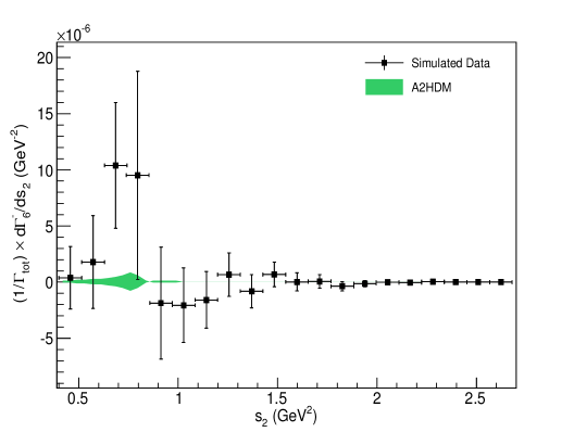
Figure 3: Projection onto $s_{2}$ of the observable $6(-)$ extracted from a set of $10^{6}$ events along with the corresponding allowed region within the A2HDM. The data in the simulation corresponds to the NP parameter choice $f_{H}\eta_{P}=1.79\,e^{i\pi/4}$. Note that the plot of the allowed region assumes that the parameters associated with the form factors ($A$, $B$, etc.) have zero uncertainty.

Inspection of Fig. 3 reveals that the distribution lies outside the A2HDM prediction only in the 3th and 4th bins, with the deviations being smaller than $2\sigma$ and almost $1\sigma$, respectively. However, as was already shown in Sec.VI.4.1, when we perform a least squares fit to this distribution with $f_{H}\eta^{I}_{P}$ as the unique free parameter, we obtain the value $1.7\pm 0.8$ (see Table 11), which is more than $2\sigma$ away from the range allowed for this parameter within the A2HDM ($|f_{H}\eta^{I}_{P}|<0.01$). Although such a deviation would cast doubt on the A2HDM in an experimental setting, it would not be enough to completely reject the model. Thus, for a NP parameter $f_{H}\eta^{I}_{P}$ two orders of magnitude above the range predicted by the A2HDM, more than $10^{6}$ events would be needed for the observable $6(-)$ to be useful in probing this model. A similar observation holds for the case of the SM, since in that case the $6(-)$ distribution is simply zero and is thus contained within the range allowed for the A2HDM. In fact, the situation here is similar to the situation that was considered in Secs. VI.2 and VI.4.1, where it was noted that more than $10^{6}$ events were required to use the $6(-)$ distribution as a tool for distinguishing between the SM and a NP scenario with $|f_{H}\eta_{P}|=1.79$.

Finally, we emphasize that the allowed region indicated in Fig. 3 assumes that the pseudoscalar form factor $f_{H}$ is a constant function of the phase space variables and that its imaginary part is zero. In order to perform a more realistic study of the A2HDM within the context of the observables discussed in this work, these assumptions would need to be tested carefully. In Sec. VIII we comment on some possibilities for testing these assumptions.

VIII Test of assumptions

As has been mentioned in previous sections, various assumptions have been made while performing the analysis in this work. Some of these assumptions could in principle be tested by using the proposed observables. In this section we describe how one could test two assumptions that have been made regarding the pseudoscalar form factor $f_{H}$; namely, that it is a flat function of $Q^{2},s_{1}$ and $s_{2}$, and that it does not contain strong phases (i.e., that $f^{I}_{H}$ is zero).

From the observables $5(-)$ and $6(-)$ in Table 3 we have the following relations

$$\frac{d\Gamma^{-}_{5}}{dQ^{2}ds_{1}ds_{2}}=\left(\frac{2}{3}A(Q^{2})\langle\overline{K}_{2}\rangle\frac{\sqrt{Q^{2}}}{m_{\tau}}B^{R}_{2}\right)\!f^{I}_{H}\eta^{I}_{P}-\left(\frac{2}{3}A(Q^{2})\langle\overline{K}_{2}\rangle\frac{\sqrt{Q^{2}}}{m_{\tau}}B^{I}_{2}\right)\!f^{R}_{H}\eta^{I}_{P}\quad\,\,\hskip 2.73148pt$$ (37)

$$\frac{d\Gamma^{-}_{6}}{dQ^{2}ds_{1}ds_{2}}=-\left(\frac{2}{3}A(Q^{2})\langle\overline{K}_{2}\rangle\frac{\sqrt{Q^{2}}}{m_{\tau}}B^{R}_{1}\right)\!f^{I}_{H}\eta^{I}_{P}+\left(\frac{2}{3}A(Q^{2})\langle\overline{K}_{2}\rangle\frac{\sqrt{Q^{2}}}{m_{\tau}}B^{I}_{1}\right)\!f^{R}_{H}\eta^{I}_{P}\,,\vspace*{2mm}$$ (38)

where we recall that the quantities $B_{1},B_{2}$ and $\langle\overline{K}_{2}\rangle$ depend on the kinematical variables $Q^{2},s_{1}$ and $s_{2}$. By projecting Eqs. (37) and (38) onto $x\equiv Q^{2},s_{1},s_{2}$ we can form a $2\times 2$ matrix equation

$$\left(\begin{array}[]{c}d\Gamma^{-}_{5}/dx\\[2.84526pt] d\Gamma^{-}_{6}/dx\end{array}\right)=\left(\begin{array}[]{rr}a_{1}&-b_{1}\\[2.84526pt] -a_{2}&b_{2}\end{array}\right)\left(\begin{array}[]{c}f^{I}_{H}\eta^{I}_{P}\\[2.84526pt] f^{R}_{H}\eta^{I}_{P}\end{array}\right),$$ (39)

where the quantities $a_{1}$ and $b_{1}$ are the projections onto $x$ of the two functions appearing inside the parentheses in Eq. (37), while $a_{2}$ and $b_{2}$ arise from the two functions in Eq. (38). Of course, these quantities are functions of $x$. Also, we note that we need to assume that $f_{H}$ has no dependence on the kinematical variables other than $x$ in order to derive Eq. (39). By inverting Eq. (39) we obtain the relations

$$f^{I}_{H}\eta^{I}_{P}=\frac{1}{a_{1}b_{2}-a_{2}b_{1}}\left(b_{2}\frac{d\Gamma^{-}_{5}}{dx}+b_{1}\frac{d\Gamma^{-}_{6}}{dx}\right)$$ (40)

$$f^{R}_{H}\eta^{I}_{P}=\frac{1}{a_{1}b_{2}-a_{2}b_{1}}\left(a_{2}\frac{d\Gamma^{-}_{5}}{dx}+a_{1}\frac{d\Gamma^{-}_{6}}{dx}\right),$$ (41)

from which we find

$$\frac{f^{I}_{H}}{f^{R}_{H}}=\frac{b_{2}\,d\Gamma^{-}_{5}/dx+b_{1}\,d\Gamma^{-}_{6}/dx}{a_{2}d\Gamma^{-}_{5}/dx+a_{1}d\Gamma^{-}_{6}/dx}.\vspace*{3mm}$$ (42)

Since we are assuming that there is no $Q^{2},s_{1}$, or $s_{2}$ dependence in $f_{H}$, the right hand side of Eq. (40) as well as of Eq. (41) must be constant over the range of $x$. Therefore, by extracting the distributions $d_{x}\Gamma^{-}_{5,6}$ from the data and obtaining the quantities $a_{1,2},b_{1,2}$ numerically for each bin in the $x$ range, the assumption regarding the flatness of $f_{H}$ (as a function of $Q^{2},s_{1}$ and $s_{2}$) can be tested. On the other hand, under the assumption that $f_{H}$ has no strong phase, the left hand side of Eq. (42) vanishes, so that the significance of the deviations from zero of the quantity appearing on the right hand side can be used to test this assumption.

Another possibility arises from the analysis of the zero-crossing points for the various distributions. Under the assumptions mentioned above, namely that $f^{I}_{H}=0$ and that its functional dependence on the kinematical variables is flat, the zero-crossing points for the $\mathrm{CP}$-odd distributions are independent of the value of the NP parameter $f_{H}\eta_{P}$. Thus, the numerical prediction of these zero-crossing points and the comparison with the distributions obtained from the data can also be used to test these two assumptions. In order to illustrate this, let us consider the

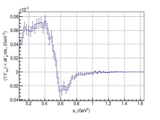
Figure 4: Projection onto $s_{1}$ of the observable $6(-)$, obtained by using a set of $3\times 10^{6}$ simulated events. The zero-crossing point can be clearly extracted from the plot with an uncertainty given by the size of the bins ($s_{1}=0.56\pm 0.03\,\,\mathrm{GeV}^{2}$).

observable $6(-)$ (see Fig. 2). Projecting this distribution separately onto $Q^{2},s_{1}$ and $s_{2}$ and performing a numerical computation of the corresponding zero-crossing points yields the values $Q^{2}\sim 1.85609\,\,\mathrm{GeV}^{2},\,s_{1}\sim 0.55633\,\,\mathrm{GeV}^{2}$ and $s_{2}\sim 0.85142\,\,\mathrm{GeV}^{2}$, respectively. On the other hand, analysis of the distributions associated with a set of $3\times 10^{6}$ events yields the following values (see Fig. 4)

$$\vspace*{2mm}Q^{2}=1.86\pm 0.04\,\,\mathrm{GeV}^{2},\quad\,s_{1}=0.56\pm 0.03\,\,\mathrm{GeV}^{2},\quad\,s_{2}=0.84\pm 0.04\,\,\mathrm{GeV}^{2},$$ (43)

which are in good agreement with the expected values. Thus, with $3\times 10^{6}$ events, it appears that one could use the zero-crossing points of the $\mathrm{CP}$-odd distributions to test the assumptions regarding $f_{H}$ that were noted above. With fewer than $3\times 10^{6}$ events, however, the zero-crossing point test would start to lose its effectiveness.

IX Conclusions

In this paper we have proposed and tested various $\mathrm{CP}$-even and $\mathrm{CP}$-odd observables for the decay $\tau\rightarrow K\pi\pi\nu_{\tau}$ by adding the contribution of a NP charged scalar to the corresponding amplitude within a model-independent approach. The various observables that we have proposed are defined in Eq. (14) (see also Tables 1 and 3). These observables are distributions that have been partially integrated over phase space, using weighting functions to pick out various terms from the original expression for the differential width (see Eq. (5)). The resulting distributions are functions of three invariant mass squared variables, $Q^{2}$, $s_{1}$ and $s_{2}$, and they depend on the NP contribution in different ways. Throughout much of the text, we have denoted the various distributions by “$i(\pm)$” $(i=1,\ldots,9$), where the “$\pm$” designation refers to whether the distribution is even (“$+$”) or odd (“$-$”) under $\mathrm{CP}$. For the numerical analysis we have used simulated events generated through our own event generator, with the maximum number of simulated events being $3\times 10^{6}$.

Among the various observables that we have proposed, the $6(-)$ distribution is the most sensitive to the NP contribution. On the one hand, for a sizeable NP contribution ($|f_{H}\eta_{P}|\sim 17.9$), we have found that this observable is useful for testing the SM hypothesis, even for $1\times 10^{5}$ events. On the other hand, the results of the fits show that this observable allows one to recover the NP parameter with the highest precision, with the uncertainties being $\lesssim\!6\,\%$ and $\lesssim\!3\,\%$ for $5\times 10^{5}$ and $3\times 10^{6}$ simulated events, respectively. More interestingly, the capability of the observable $6(-)$ to recover the NP parameter is not spoiled when the size of the NP contribution is reduced.

Regarding the $\mathrm{CP}$-even observables that we study in this paper, we have found that the $5(+)$ distribution and the $s_{1,2}$ projections of the $7(+)$ distribution show the most promise for recovering the parameter $A$, which is related to the weight of the resonant contributions. Additionally, considering that the $8(+)$ and $9(+)$ distributions extracted from the set of $3\times 10^{6}$ simulated events are consistent with zero to within their statistical uncertainties, we have shown that the observable $5(+)$ is the most suitable alternative for extracting information about the anomalous Wess-Zumino term once the other parameters related to the various resonances have been measured.

The results involving the $\mathrm{CP}$-odd observables have been derived under the assumptions that $f^{I}_{H}=0$ and that its functional dependence on the kinematical variables is flat. The same assumptions have been made for the $\mathrm{CP}$-even observables, but in that case, we have also assumed that $F_{4}=0$. The possibilities for testing some of these assumptions by using the observables defined in this paper have been discussed in Sec.VIII.

We have also studied the decay $\tau\rightarrow K\pi\pi\nu_{\tau}$ within the context of the A2HDM and have found that the observables that we have defined may be used to test this model. In particular, we have focused on the $s_{2}$ projection of the differential width $6(-)$, comparing the range allowed by the A2HDM to that predicted by our simulation, adopting the NP parameter choice $|f_{H}\eta_{P}|=1.79$. Using a simulation with $10^{6}$ events, we have found that the best fit value for $f_{H}\eta^{I}_{P}$ obtained from the distribution is in disagreement (by more than $2\sigma$) with the range predicted for the A2HDM. With the NP parameter choice $|f_{H}\eta_{P}|=17.9$ and the same number of events, the disagreement between the two scenarios is much greater and one would be able to distinguish decisively between them.

We note that a similar set of observables could be defined in order to analyze other decay modes such as $\tau^{-}\rightarrow\pi^{-}\pi^{+}\pi^{-}\nu_{\tau},\,\tau^{-}\rightarrow K^{-}K^{+}\pi^{-}\nu_{\tau}$ and $\tau^{-}\rightarrow K^{-}K^{+}K^{-}\nu_{\tau}$, and their $\mathrm{CP}$-conjugated decays. In fact, precise measurements of the branching ratios for these decays have already been obtained at the B-factories (see Refs. Aubert et al. (2008); Adachi et al. for example).

An experimental analysis of the observables we have analyzed in this paper could be useful not only for extracting information about the resonance structure of the decay $\tau\rightarrow K\pi\pi\nu_{\tau}$ but also for obtaining additional constraints on the NP pseudoscalar coupling. Moreover, with the higher luminosity expected for the upcoming Super B-factories, the number of events anticipated for the decay $\tau\rightarrow K\pi\pi\nu_{\tau}$ would be enough to exploit the information provided by the proposed observables.

Acknowledgments The authors wish to acknowledge helpful discussion and communication with S. Banerjee, I. Nugent, M. Roney and G. Valencia. They also wish to thank C. Daudt, N. Lickey and N. White for technical assistance, and A. Pich for revising the manuscript. This work has been partially supported by ANPCyT under grant No. PICT-PRH 2009-0054 and by CONICET (NM, AS). The work of KK was supported by the U.S. National Science Foundation under Grant PHY-1215785. KK also acknowledges sabbatical support from Taylor University.

Appendix A Statistical Uncertainties

In this appendix we summarize some results regarding statistical uncertainties associated with the distributions considered in this work.

The estimator that we have used to extract the projections onto $Q^{2},s_{1}$, and $s_{2}$ of the weighted partial differential widths from the simulated events is given by:

$$\frac{1}{\Gamma_{\mathrm{tot}}}\frac{\hat{d\Gamma}_{i}}{dx}(x_{0})=\frac{N}{N_{\mathrm{ev}}}\frac{\bar{h}_{i}}{\Delta x}\mathcal{B}_{\tau\rightarrow K\pi\pi\nu_{\tau}}\,,$$ (44)

where $\frac{\hat{d\Gamma}_{i}}{dx}(x_{0})$ denotes the projection onto $x\equiv Q^{2},s_{1},s_{2}$ of the $i$-th weighted partial width evaluated at $x_{0}$, $N$ is the number of events within the bin $(x_{0}-\Delta x/2,x_{0}+\Delta x/2)$, $\bar{h}_{i}$ is the sample mean of the angular function $h_{i}(\gamma,\beta)$ (see Table 1) in the bin and $N_{\mathrm{ev}}$ is the total number of simulated events. We note that the presence of the branching ratio ($\mathcal{B}_{\tau\rightarrow K\pi\pi\nu_{\tau}}$) arises from the fact that we have normalized the observables to the total decay width ($\Gamma_{\mathrm{tot}}$).

In order to estimate the statistical error associated with $d\Gamma_{i}/dx$, we use error propagation in Eq. (44), taking into account the standard deviations of the number of events in a given bin, $N$, and of the sample mean $\bar{h}_{i}$. The expression that we obtain for the $j$-th bin is given by:

$$\sigma_{j}=\frac{\mathcal{B}_{\tau\rightarrow K\pi\pi\nu_{\tau}}}{\Delta x}\frac{\sqrt{I_{j}}}{\sqrt{N_{\mathrm{ev}}}}(\sigma_{h_{i}}+\langle h_{i}\rangle\sqrt{1-I_{j}}),$$ (45)

where $\sigma_{h_{i}}=\sqrt{\langle h^{2}_{i}\rangle-\langle h_{i}\rangle^{2}}$ is the standard deviation of $h_{i}$ computed for the $j$-th bin, $I_{j}$ is the probability for a given event to lie within that bin and $\langle h^{2}_{i}\rangle$ and $\langle h_{i}\rangle$ denote the mean values of $h^{2}_{i}$ and $h_{i}$, respectively, which are calculated, again, for the $j$-th bin. In general, for all the observables the dominant contribution arises from the standard deviation of the angular function, $\sigma_{h_{i}}$, while the second term in Eq. (45) is negligible. The unique exception is the observable with $i=1$, for which $\sigma_{h_{1}}=0$ (due to the fact that $h_{1}(\alpha,\beta)=1$ – see Table 1), so that the second term is the dominant one. Actually, this second term computed for the observable $d\Gamma_{1}/dx$ turns out to be comparable to the first contribution obtained for any of the remaining observables ($d\Gamma_{i}/dx,\,i=2,\ldots,9$). Therefore, the statistical uncertainties $\sigma_{j}$ are of the same order of magnitude for all of the weighted partial widths ($i=1,\ldots,9$). Of course, the order of magnitude of the uncertainty in Eq. (45) changes from one bin to another and from one projection to another ($x=\,Q^{2},s_{1}$ or $s_{2}$).

References