Stress tensor and current correlators of interacting conformal field theories in 2+1 dimensions: Fermionic Dirac matter coupled to $U(1)$ gauge field

Abstract

We compute the central charge $C_{T}$ and universal conductivity $C_{J}$ of $N_{F}$ fermions coupled to a $U(1)$ gauge field up to next-to-leading order in the $1/N_{F}$ expansion. We discuss implications of these precision computations as a diagnostic for response and entanglement properties of interacting conformal field theories for strongly correlated condensed matter phases and conformal quantum electrodynamics in $2+1$ dimensions.

I Introduction

A variety of strongly correlated electron systems at quantum critical points or phases in two spatial dimensions are believed to be described by (interacting) conformal field theories in 2+1 dimensions (CFT₃’s). The workhorse is the Wilson-Fisher CFT₃, also known as the $O(N)$-model of a real-valued vector field with $N$ components wilsonfisher71 ; abe73 ; petkou95 , which describes, among other things, the Ising model for $N=1$ showk12 ; showk14 , superfluid-to-insulator transitions for $N=2$ cha91 ; fazio96 , and quantum magnetic transitions for $N=3$ nelson89 ; chubukov94 . Especially intriguing are gauge theoretical descriptions of condensed matter systems (e.g.: kaul08 and references therein for an overview) such as of quantum Hall systems (e.g.: chen92 ; chen93 and references therein), fractionalized magnets and deconfined critical points in strongly correlated Mott insulators senthil04 ; sandvik07 ; huhprl13 , and effective theories for the cuprates rantner02 ; franz02 ; franz03 ; kaul07 . There, the relevant dynamics is often provided by emergent or effective degrees of freedom not necessarily present in the bare Hamiltonian. These conformal phases of quantum matter in 2+1 dimensions provide a unique interpolation between the better understood CFT’s in 1+1 dimensions cardy08 and much studied gauge theories for high energy vacua in 3+1 dimensions polyakov87 ; coleman88 .

A common feature of CFT₃’s is the absence of quasi-particles and for condensed matter systems it is of particular interest to understand response properties of interacting CFT₃’s to externally applied perturbations such as electromagnetic fields or mechanical forces without invoking a quasi-particle picture.

I.1 Model: $N_{F}$ Dirac fermions coupled to $U(1)$ gauge field

In this paper, we consider $N_{F}$ Dirac fermions minimally coupled to a $U(1)$ gauge field. This theory arises in a variety of condensed matter contexts kaul08 ; chen93 ; rantner02 ; franz02 ; kaul07 . The Euclidean action,

$$\mathcal{S}=\int d^{2}rd\tau\bar{\psi}_{\alpha}\left[i\gamma^{\mu}\left(\partial_{\mu}-i\frac{A_{\mu}}{\sqrt{N_{F}}}\right)\right]\psi_{\alpha}+...\;,$$ (1)

contains Grassmannian two-component fermion fields $\bar{\psi}_{\alpha}$ and $\psi_{\alpha}$, where $\alpha$ is the fermion flavor index, and $\mu$ is the spatial and (imaginary) temporal index in $2+1$ dimensions. Repeated indices are summed over. $\gamma^{\mu}$’s are the Dirac matrices that satisfy $\{\gamma^{\mu},\gamma^{\nu}\}=2\delta^{\mu\nu}$. We use the same conventions as Kaul and Sachdev for their fermion sector kaul08 . The dots stand for additional terms which may play a role in the UV and away from the conformally invariant fixed-point considered in this paper.

The gauge field $A_{\mu}$, a conventional spin-1 boson often dubbed as “emergent photon” in the condensed matter context, ensures fulfillment of a local $U(1)$ gauge symmetry at every point $(\tau,\mathbf{r})$ in (Euclidean) space-time. A potential, bare Maxwell term $\frac{1}{2e^{2}}F_{\mu\nu}F^{\mu\nu}$ is not written in Eq. (1) and is unimportant for the universal constants at the infrared fixed point of interest in this paper klebanov12 . The gauge field gets dynamical by integrating the fermion fields in the large $N_{F}$ limit. In Landau gauge, the gauge field propagator at $N_{F}\rightarrow\infty$ is purely transverse and takes the characteristic overdamped form (with $p=|{\bm{p}}|$)

$$D^{(0)}_{\mu\nu}(p)=\frac{16}{p}\left(\delta_{\mu\nu}-\frac{p_{\mu}p_{\nu}}{p^{2}}\right)\;.$$ (2)

Model Eq. (1) with a bare Maxwell term is also known as QED₃ and flows to strong coupling in the infrared and shares its propensity to form fermion bound states “mesons” with QCD in 3+1 dimensions appelquist86 ; appelquist88 ; nash89 . Deforming QED₃ toward graphene-type models with instantaneous Coulomb interactions are also interesting son07 ; juricic10 ; herbut13 ; kotikov14 ; barnes14 . It is believed that for sufficiently large $N_{F}$, Eq. (1) flows to a strongly coupled conformal phase in the infrared, preserving scale invariance braun14 (and references therein).

I.2 Key results: central charge $C_{T}$ and $C_{J}$ up to next-to-leading order in $1/N_{F}$

The main result of this paper is an explicit formula and numerical value of the central charge $C_{T}$ of Eq. (1), defined below as the universal constant appearing in the stress tensor correlator at the interacting conformal fixed point, up to next-to-leading order in the $1/N_{F}$ expansion:

$$\frac{C_{T}}{N_{F}}= \frac{1}{256}\left(1+\frac{1}{N_{F}}\left(\tilde{C_{T}}^{(1)}+\frac{104}{15\pi^{2}}\right)\right)\;$$

$$= \frac{1}{256}\left(1+\frac{0.28701185900024704065}{N_{F}}\right)\;.$$ (3)

$\tilde{C_{T}}^{(1)}$ comes from one out of nine Feynman graphs in momentum space computed below in Fig. (5)

$$\tilde{C_{T}}^{(1)} =-\frac{4}{45\pi^{2}}\Bigg{(}180\text{Li}_{2}\left(3-2\sqrt{2}\right)-720\text{Li}_{2}\left(-1+\sqrt{2}\right)-398+90\pi^{2}+45\log^{2}\left(3-2\sqrt{2}\right)$$

$$~{}~{}~{}~{}~{}~{}~{}~{}~{}~{}~{}~{}~{}~{}~{}~{}+1146\sqrt{2}\log\left(3-2\sqrt{2}\right)+12\left(191\sqrt{2}+15\log\left(3-2\sqrt{2}\right)\right)\sinh^{-1}(1)\Bigg{)}$$

$$=~{}-0.41548168091996150803\;,$$ (4)

where Li${}_{n}(z)=\sum_{k=1}^{\infty}\frac{z^{k}}{k^{n}}$ is the polylogarithm or Jonquiére’s function for $n=2$. The sum of other eight diagrams evaluate to the remaining term in the innermost bracket, $\frac{104}{15\pi^{2}}$, in the first line of Eq. (3). We observe from Eq. (3) that $1/N_{F}$ corrections to the $N_{F}\rightarrow\infty$ value are $\approx 15\%$ when $N_{F}=2$. Even larger $1/N$ corrections were observed (for current correlators) in the $CP^{N-1}$ model and attributed in particular to vertices directly involving the gauge field huh13_long .

It is interesting to note that here in Eq. (3) the $1/N_{F}$ corrections are positive whereas in certain theories with bosonic field content huhprl13 ; huh13_long ; petkou94 ; petkou95 ; petkou96 the $1/N_{B}$ corrections to $C_{T}$ as well as $C_{J}$ (see below) typically turn out to be negative. Given this information, the sign of the correction could be attributed to the quantum statistics of the charged fields but further analysis (see also conclusions for an outlook ondual Chern-Simons + matter theories) and potentially higher-order computations are needed to uncover further the structure of these corrections.

It is hard to overestimate the fundamental importance of the central charge in conformal field theory with applications ranging from thermodynamics, quantum critical transport, to quantum information theory cardy10 . An interesting recent application are explicit formulae for the Rényi entropy for $d$-dimensional flat space CFT’s and we quote here the formula from Perlmutter perlmutter14 :

$$S^{\prime}_{q=1}=-{\rm{Vol}}\left(\mathbb{H}^{d-1}\right)\frac{\pi^{d/2+1}\Gamma(d/2)(d-1)}{(d+1)!}C_{T}\;.$$ (5)

The prime denotes a derivative with respect to $q$ of the Rényi entropy $S_{q}=\frac{1}{1-q}\log{\rm Tr}\left[\rho^{q}\right]$, $\rho$ a reduced density matrix, and $\mathbb{H}^{d-1}$ the hyperboloid entangling surface. Moreover, precision values of $C_{T}$ may be useful for conformal bootstrap approaches for the 3D-Ising and other models showk12 as well as serving as a benchmark for numerical simulations of frustrated quantum magnets kaul13 .

In the present paper, we compute $C_{T}$ by direct evaluation of Feynman graphs in momentum space fulfilling and using the relation cardy87 ; chowdhury13 ,

$$\langle T_{\mu\nu}(-p)T_{\lambda\rho}(p)\rangle=C_{T}|{\bm{p}}|^{3}\Bigg{(} \delta_{\mu\lambda}\delta_{\nu\rho}+\delta_{\mu\rho}\delta_{\nu\lambda}-\delta_{\mu\nu}\delta_{\lambda\rho}+\delta_{\mu\nu}\frac{p_{\lambda}p_{\rho}}{p^{2}}+\delta_{\lambda\rho}\frac{p_{\mu}p_{\nu}}{p^{2}}-\delta_{\mu\lambda}\frac{p_{\nu}p_{\rho}}{p^{2}}-\delta_{\nu\lambda}\frac{p_{\mu}p_{\rho}}{p^{2}}$$

$$-\delta_{\mu\rho}\frac{p_{\nu}p_{\lambda}}{p^{2}}-\delta_{\nu\rho}\frac{p_{\mu}p_{\lambda}}{p^{2}}+\frac{p_{\mu}p_{\nu}p_{\lambda}p_{\rho}}{p^{4}}\Bigg{)}\;$$ (6)

generalizing our recently developed technology huhprl13 ; huh13_long to Dirac fermions and contractions over stress tensor vertices. We discuss this further in Sec. IV.

Computations of stress tensor correlators in interacting CFT’s (at least without an excessive amount of symmetry such as supersymmetries) in effective dimensionality greater than 2 are extremely scarce and we are not aware of a previous computation of $C_{T}$ for Eq. (1) in 2+1 dimensions. We quote here related works across the quantum field theory universe we are aware of to date: two papers by Hathrell using loop expansions from 1982, one on scalar fields up to 5-loops hathrell_scalar and one on QED up to 3 loops hathrell_qed , a two-loop analysis for general gauge theories coupled to fermions and scalars in curved space by Jack and Osborn in 1984 and 1985 jack84 ; jack85 , an $\epsilon$-expansion around four dimensions for scalar and gauge theories by Cappelli, Friedan and LaTorre in 1991 cappelli91 , and a series of papers on the $O(N)$ vector model from 1994-1996 by Petkou and Osborn petkou94 ; petkou95 ; petkou96 , and a three-loop OPE computation in massless QCD by Zoller and Chetyrkin in 2012 zoller12 .

For essentially free field theories, stress tensor amplitudes maldacena11 ; chowdhury13 and Rényi entropies klebanov12 have also been computed. (Multi-point) correlators of the stress tensor are also instrumental for the relation between scale and conformal invariance (e.g.: dymarsky13 ; bzowski14 ). It would be interesting to consider generalizations of Eq. (1) with conformally invariant UV fixed points to be able to compare $C_{T}^{IR}$ and $C_{T}^{UV}$ for a given number of flavors in the context of generalized c-theorems for CFT’s in general dimensions myers11 ; klebanov11 ; appelquist99 . It is known that QED₃, including a Maxwell term $\frac{1}{2e^{2}}F^{2}$, flows toward a weakly interacting UV fixed-point. Against this backdrop, an assessment of the full conformal symmetry (free photons are not necessarily conformally invariant in the UV), and a systematic investigation of possible UV fixed points and their relevant operators is an interesting extension of our work.

The second result of this paper is an (somewhat simpler) computation of the universal constant $C_{J}$ of the two-point correlator of the conserved flavor current of Eq. (1):

$$J^{\ell}_{\mu}=\bar{\psi}_{\alpha}T^{\ell}_{\alpha\beta}\gamma_{\mu}\psi_{\beta}\;,$$ (7)

where $T^{\ell}$’s are generators of the SU$(N_{F})$ group normalized to satisfy $\text{Tr}(T^{\ell}T^{m})=\delta^{\ell m}$. As the stress tensor $T_{\mu\nu}$, this flavor current is conserved and its two-point correlator depends on one universal constant $C_{J}$

$$\langle J^{\ell}_{\mu}(-p)J^{m}_{\nu}(p)\rangle=-C_{J}|{\bm{p}}|\left(\delta_{\mu\nu}-\frac{p_{\mu}p_{\nu}}{p^{2}}\right)\delta^{\ell m}\;.$$ (8)

For single fermion QED₃, $C_{J}$ describes the universal electrical conductivity in the collisionless regime $\omega\gg T$, with $T$ being the temperature. Depending on the physical context, however, it may also be related to magnetic or other response functions rantner02 . Our result for $C_{J}$ to next-to-leading order in $1/N_{F}$ is (derived in Sec. II)

$$C_{J}= \frac{1}{16}\left(1+\frac{1}{N_{F}}\left(\tilde{C_{J}}^{(1)}-\frac{40}{9\pi^{2}}\right)\right)$$

$$= \frac{1}{16}\left(1+\frac{1}{N_{F}}0.14291062004225554348\right)\;$$ (9)

with the analytical expression corresponding to one of the graphs being

$$\tilde{C_{J}}^{(1)}= -\frac{4}{3\pi^{2}}\Bigg{(}-34+6\pi^{2}+\sinh^{-1}(1)\left(52\sqrt{2}+6\log\left(17-12\sqrt{2}\right)\right)+26\sqrt{2}\log\left(3-2\sqrt{2}\right)$$

$$+3\log^{2}\left(3-2\sqrt{2}\right)+24\text{Li}_{2}\left(1-\sqrt{2}\right)-24\text{Li}_{2}\left(-1+\sqrt{2}\right)\Bigg{)}$$

$$= ~{}0.59322699178597897212\;.$$ (10)

As for $C_{T}$, we again find the $1/N_{F}$ corrections to $C_{J}$ to be positive in contrast to the bosonic field theories analyzed in Ref. huhprl13, ; huh13_long, . Our numerical value of the correction is seemingly in disagreement with the value computed in the Appendix of Ref. chen93, and we compare to their value in detail in Sec. II. As a (positive) cross-check, we have repeated a different calculation of the (non-conserved) staggered spin susceptibility in the Appendix of Rantner and Wen rantner02 using our approach and found the same logarithmically divergent coefficients.

Note that Eq. (1) has a further conserved “topological” current related to the curl of the gauge field chowdhury13 but we do not consider it further here.

I.3 Organization of paper

The remainder of the paper is organized as follows: in Sec. II, we define the Feynman rules for Eq. (1) and the current vertex, and evaluate the 3 graphs renormalizing the current-current correlator. In Sec. III, we briefly recapitulate the main elements of the Tensoria technology for the momentum integrals. In Sec. IV, we define the stress tensor vertex and evaluate the 9 graphs renormalizing the stress tensor correlator. In the conclusions, we summarize and point toward potential future directions where our technology could be applied to.

II Flavor current correlator $\langle JJ\rangle$

In this section, we compute the SU$(N_{F})$ flavor current-current correlator and compare it to the previous computation also using the $1/N_{F}$ expansion that we are aware of chen93 . We begin by stating the Feynman rules, compute the leading $N_{F}\rightarrow\infty$ graph in some detail, and then the more complicated self-energy and vertex corrections at order $1/N_{F}$. We will separate the contributions into longitudinal and transverse projections and show that all longitudinal and logarithmically singular corrections mutually cancel as they should for a conserved, transverse quantity.

II.1 Feynman rules and graphs in momentum space

The Feynman rules for $N_{F}$ Dirac fermions coupled to $U(1)$ gauge field in Eq. (1) contain the relativistic fermion propagator

$$G_{\psi}(k)=\frac{k_{a}\gamma_{a}}{k^{2}}\;,$$ (11)

the gauge field propagator in Eq. (2), and the photon-fermion vertex drawn in Fig. 1.

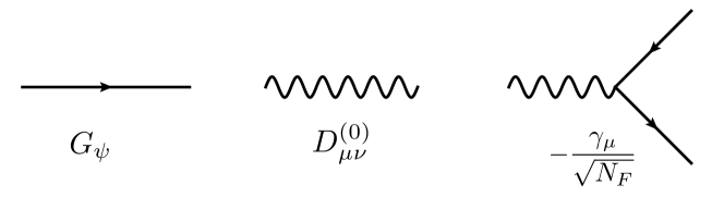
Figure 1: Feyman rules for $N_{F}$ Dirac fermions coupled to $U(1)$ gauge field in Eq. (1).

The current vertex in Fig. 2 involves one generator of the SU$(N_{F})$ but the traces over them in the actual diagrams are innocuous and just give $\delta$-functions in the flavor indices.

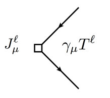
Figure 2: Feyman rule for the current vertex. $T^{\ell}$ is a generator of the SU$(N_{F})$.

Using the Feynman rules explained above, Fig. 3 exhibits the 3 contractions to the current correlator to order $1/N_{F}$. Each of the expressions in Eq. 12 contain a minus sign due to the trace over fermions, a (trivial) trace over flavor indices, a trace over the Dirac matrices, and one (1-loop graph) or two (the two 2-loop graphs) $2+1$ dimensional momentum integrals $\int_{{\bm{k}}}\equiv\int\frac{d^{3}k}{8\pi^{3}}$.

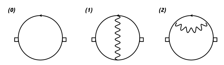
Figure 3: Feyman diagrams contributing to the current current correlator to order $1/N_{F}$. Diagram (0) is the leading order contribution and the only one that survives the $N_{F}\rightarrow\infty$ limit. Diagram (1) is the vertex correction, diagram (2) the self-energy correction that comes with a factor of $a_{2}=2$.

We get:

$$J_{\mu\nu}^{\ell m}(p)^{(0)} =-\text{Tr}\left[\int_{\bm{k}}\gamma_{\nu}T^{m}\frac{k_{a}\gamma_{a}}{k^{2}}\gamma_{\mu}T^{\ell}\frac{({\bm{p}}+{\bm{k}})_{b}\gamma_{b}}{({\bm{p}}+{\bm{k}})^{2}}\right]$$ (12)

$$J_{\mu\nu}^{\ell m}(p)^{(1)} =-\text{Tr}\left[\int_{{\bm{k}},{\bm{q}}}\gamma_{\nu}T^{m}\frac{({\bm{k}}+{\bm{p}})_{a}\gamma_{a}}{({\bm{k}}+{\bm{p}})^{2}}\frac{\gamma_{\lambda}}{\sqrt{N_{F}}}\frac{({\bm{k}}+{\bm{p}}+{\bm{q}})_{b}\gamma_{b}}{({\bm{k}}+{\bm{p}}+{\bm{q}})^{2}}\gamma_{\mu}T^{\ell}\frac{({\bm{k}}+{\bm{q}})_{c}\gamma_{c}}{({\bm{k}}+{\bm{q}})^{2}}\frac{\gamma_{\rho}}{\sqrt{N_{F}}}\frac{k_{d}\gamma_{d}}{k^{2}}\frac{16}{q}\left(\delta_{\lambda\rho}-\frac{q_{\lambda}q_{\rho}}{q^{2}}\right)\right]$$

$$J_{\mu\nu}^{\ell m}(p)^{(2)} =-\text{Tr}\left[\int_{{\bm{k}},{\bm{q}}}\gamma_{\nu}T^{m}\frac{({\bm{k}}+{\bm{p}})_{a}\gamma_{a}}{({\bm{k}}+{\bm{p}})^{2}}\gamma_{\mu}T^{\ell}\frac{k_{b}\gamma_{b}}{k^{2}}\frac{\gamma_{\rho}}{\sqrt{N_{F}}}\frac{({\bm{k}}+{\bm{q}})_{c}\gamma_{c}}{({\bm{k}}+{\bm{q}})^{2}}\frac{\gamma_{\lambda}}{\sqrt{N_{F}}}\frac{k_{d}\gamma_{d}}{k^{2}}\frac{16}{q}\left(\delta_{\lambda\rho}-\frac{q_{\lambda}q_{\rho}}{q^{2}}\right)\right]\;.$$

These expressions are now evaluated in the following way using our “Tensoria” technology huh13_long : We first perform the trace over the Dirac indices, collecting the contracted expressions in the numerator. Especially for the more complicated expressions it is helpful to automate it and use the Feyncalc MATHEMATICA package for this feyncalc . Then we replace the integrals of momentum written in components as described in the next section and in the Appendix of Ref. huh13_long, . Finally, we separate out the transverse $I^{(i)}_{\text{T}}$ and longitudinal $I^{(i)}_{\text{T}}$ momentum projections in the following form:

$$\langle J^{\ell}_{\mu}(-p)J^{m}_{\nu}(p)\rangle =\delta^{\ell m}\sum_{i=0}^{2}a_{i}J^{(i)}_{\mu\nu}(p)\equiv\sum_{i=0}^{2}a_{i}\left[I^{(i)}_{\text{T}}(p)\left(\delta_{\mu\nu}-\frac{p_{\mu}p_{\nu}}{p^{2}}\right)+I^{(i)}_{\text{L}}(p)\frac{p_{\mu}p_{\nu}}{p^{2}}\right]\;.$$ (13)

II.2 Free fermion limit, $N_{F}\rightarrow\infty$ graph, for $C_{J}$

To illustrate the procedure with a simple example, let us evaluate the leading order graph that also corresponds to the free fermion limit:

$$J_{\mu\nu}^{\ell m}(p)^{(0)} =-\text{Tr}\left[\int_{\bm{k}}\gamma_{\nu}T^{m}\frac{k_{a}\gamma_{a}}{k^{2}}\gamma_{\mu}T^{\ell}\frac{({\bm{p}}+{\bm{k}})_{b}\gamma_{b}}{({\bm{p}}+{\bm{k}})^{2}}\right]$$

$$=\delta^{\ell m}\int\frac{d^{3}k}{8\pi^{3}}\frac{2k^{2}\delta_{\mu\nu}+2\delta_{\mu\nu}k_{\alpha}p_{\alpha}-4k_{\mu}k_{\nu}-2k_{\nu}p_{\mu}-2k_{\mu}p_{\nu}}{k^{2}\left({\bm{p}}+{\bm{k}}\right)^{2}}\;.$$ (14)

The integral over the first term in the numerator $2k^{2}\delta_{\mu\nu}$ is a power-law divergence in the UV and can be dropped. The second, third, fourth and firth term in the numerator can be integrated using the identities

$$\int\frac{d^{3}k}{8\pi^{3}}\frac{k_{\mu}}{k^{2}\left({\bm{p}}+{\bm{k}}\right)^{2}} =-\frac{p_{\mu}}{16p}$$

$$\int\frac{d^{3}k}{8\pi^{3}}\frac{k_{\mu}k_{\nu}}{k^{2}\left({\bm{p}}+{\bm{k}}\right)^{2}} =\left(3\frac{p_{\mu}p_{\nu}}{p^{2}}-\delta_{\mu\nu}\right)\frac{p}{64}$$ (15)

with the abbreviation for the modulus $p=|{\bm{p}}|$ and interchangebly $p^{2}={\bm{p}}^{2}$. The result

$$J_{\mu\nu}^{\ell m}(p)^{(0)} =-\frac{p}{16}\left(\delta_{\mu\nu}-\frac{p_{\mu}p_{\nu}}{p^{2}}\right)\delta^{\ell m}$$ (16)

comes out purely transverse, leading to $C_{J}^{N_{f}\rightarrow\infty}=1/16$. Note that in order to compute $\langle TT\rangle$ (in the next section), Tensoria performs momentum integrals of the type Eq. (15) containing up to six different momentum indices in the numerator and four propagators in the denominator.

II.3 $1/N_{F}$ corrections to $C_{J}$ and discussion

We evaluate the vertex correction and self-energy correction graphs (1) and (2) in Eq. 12 algorithmically and the results are in Table 1. As expected for a conserved quantity, the log-singularities of each individual graph cancel when taking the sum, so does the longitudinal part.

Diagram	$I_{T}^{(i)}(p)$	$I_{L}^{(i)}(p)$	Log-Singularity (transverse)	Factor $a_{i}$
0	$-\frac{1}{16}p$	0	0	1
1	$-\frac{p}{N_{F}}0.0370767$	$\frac{p}{N_{F}}\frac{1}{3\pi^{2}}$	$\frac{p}{N_{F}}\frac{2}{3\pi^{2}}\log{\frac{\Lambda}{p}}$	1
2	$\frac{p}{N_{F}}\frac{5}{36\pi^{2}}$	$-\frac{p}{N_{F}}\frac{1}{6\pi^{2}}$	$-\frac{p}{N_{F}}\frac{1}{3\pi^{2}}\log{\frac{\Lambda}{p}}$	2

Table 1: Evaluated contributions to the current-current correlator. The sum of longitudinal components off all the graphs add to 0 and the transverse parts add up to Eq. (9). The analytic expression for $I^{(1)}_{T}(p)$ (multiplied by -16) is in Eq. (10) The log-singularities mutually cancel. The self-energy correction graph (2) comes with a factor of $a_{2}=2$.

As announced in the Introduction, our result Eq. (9) seems to disagree with Chen et al.chen93 who computed $C_{J}$ for QED₃ to order $1/N_{F}$. The relevant $1/N_{F}$ correction is given in Eq. (A17) in the appendix of their paper. Mapping to our conventions we take $g=1$ and $A=16$ and an overall minus sign. These authors obtained

$$C^{\text{Chen, et al.}}_{J}=\frac{1}{16}\left(1+\frac{16}{N_{F}}\frac{3}{(2\pi)^{2}}\right)\approx\frac{1}{16}\left(1+\frac{1}{N_{F}}1.216\right)\;,$$ (17)

The sign of their $1/N_{F}$ correction match but the value seem to be different from Eq. (9). As another, this time positive, cross-check, we have repeated the calculation of Appendix B in the paper by Rantner and Wen rantner02 and compared the coefficients of the logarithmically diverging terms in their Eq. (B10) to what we get. Both values agree to be

$$-\frac{1}{N_{F}}\frac{16}{3\pi^{2}}|\mathbf{p}|\ln\frac{\Lambda}{|\mathbf{p}|}\;.$$ (18)

The presence of (non-cancelling) log-singularities indicates that the quantity (staggered spin susceptibility in algebraic spin liquids) in their case is not conserved. We have also computed the fermion anomalous dimension and self energy correction to order $1/N_{F}$ and found agreement to results from direct calculation using textbook methods (See Ref. franz02, ).

III Tensoria technology: mini-recap

Before proceeding, let us briefly recapitulate our algorithm to evaluate the tensor-valued momentum integrals as described in more detail in the Appendices of huh13_long ; bzowski12 . At the heart of the algorithm are Davydychev permutation davydychev91 ; davydychev92 relations to perform integrals of the form:

$$J_{\mu_{1}...\mu_{M}}\left({\bm{p}}_{1},{\bm{p}}_{2},{\bm{p}}_{3};n;{\nu_{i}}\right)=\int d^{n}{{\bm{k}}}\frac{k_{\mu_{1}}...k_{\mu_{M}}}{\left({\bm{k}}+{\bm{p}}_{1}\right)^{2\nu_{1}}\left({\bm{k}}+{\bm{p}}_{2}\right)^{2\nu_{2}}\left({\bm{k}}+{\bm{p}}_{3}\right)^{2\nu_{3}}}\;.$$ (19)

After the Dirac traces, the integrals can all be brought into this form. After the first momentum integration, we temporarily introduce a UV-momentum cutoff that formally breaks symmetries such as conformal invariance. Using this cutoff as a sorter, all power-law divergences are discarded as they would be absent in a gauge-invariant regularization schemes such as dimensional regularization. The remaining finite and logarithmically divergent terms can be integrated analytically graph-by-graph and the log-singularities are seen to cancel exactly.

We close this recap by noting that despite the exact cancellations of the log-singularities as a strong consistency check, and the many additionally performed checks of all sub-routines in Tensoria, at the moment we have no proof that of the exactness to $O(1/N_{F})$ of our results for the theory Eq. (1). Note that the Tensoria technique was also applied in Refs. huhprl13, ; huh13_long, , for different theories. There, we found agreement with a number of computations using other methods.

IV Stress energy tensor correlator $\langle TT\rangle$

In this section, we extend our technology to compute the stress tensor correlator of Eq. (1) to next-to-leading order in $1/N_{F}$. We first define the stress tensor itself and write down the Feynman rules for the stress tensor vertices. Then, we first illustrate in some detail the calculation of the leading $N_{F}\rightarrow\infty$ graph before evaluating the remaining 8 graphs with Tensoria. The two major complications here are: (i) the gauge field can connect directly to the stress tensor vertex leading to a vertex involving 3 lines, and (ii) four 3-loop graphs, including those of the Azlamasov-Larkin type, appear. As in the $\langle JJ\rangle$ computation, we explicitly show that all log-singularities cancel when summing all graphs to ensure to conserved nature of $T_{\mu\nu}$ in accordance with symmetries.

IV.1 Feynman rules and graphs in momentum space

The stress tensor operator for Eq. (1) depends on both the fermions and the gauge fields via the gauge covariant derivative $D_{\mu}=\partial_{\mu}-iA_{\mu}/\sqrt{N_{F}}$ chowdhury13

$$T_{\mu\nu}=\sum_{\alpha=1}^{N_{F}}\frac{i}{4}\left(\bar{\psi_{\alpha}}\gamma_{\mu}\left(D_{\nu}\psi_{\alpha}\right)+\bar{\psi}_{\alpha}\gamma_{\nu}\left(D_{\mu}\psi_{\alpha}\right)-\left(D^{\ast}_{\mu}\bar{\psi_{\alpha}}\right)\gamma_{\nu}\psi_{\alpha}-\left(D^{\ast}_{\nu}\bar{\psi_{\alpha}}\right)\gamma_{\mu}\psi_{\alpha}\right)\;.$$ (20)

leading to the stress tensor vertices shown in Fig. 4.

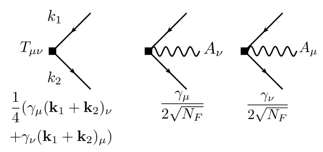
Figure 4: Feyman rules for the stress tensor vertices.

The eight graphs and their analytical expressions shown in Figs. 5, 6 contribute to order $1/N_{F}$ and we again denote their sum by

$$\langle T_{\mu\nu}(-p)T_{\lambda\rho}(p)\rangle =\sum_{i=0}^{7}a_{i}T^{(i)}_{\mu\nu\lambda\rho}(p)\;.$$ (21)

Figure 5: Feynman diagrams contributing to the stress energy tensor correlator to next-to-leading order in $1/N_{F}$. Only diagram (0) survives in the $N_{F}\rightarrow\infty$ limit. Diagrams (2) and (4) come with a factor of $a_{2}=2$, $a_{4}=2$, respectively. The factors for the other graphs are unity $a_{i}=1$. The numerical values and logarithmic singularities for each of these graphs are exhibited in Table 2.

$$T_{\mu\nu\lambda\rho}^{(0)}(p) =-N_{F}\text{Tr}\left[\int_{\bm{k}}\frac{1}{4}\gamma_{\lambda}(2{\bm{k}}+{\bm{p}})_{\rho}\frac{({\bm{k}}+{\bm{p}})_{a}\gamma_{a}}{({\bm{k}}+{\bm{p}})^{2}}\frac{1}{4}\gamma_{\mu}(2{\bm{k}}+{\bm{p}})_{\nu}\frac{k_{b}\gamma_{b}}{k^{2}}\right]+(\text{perm1})$$

$$T_{\mu\nu\lambda\rho}^{(1)}(p) =-N_{F}\text{Tr}\Bigg{[}\int_{{\bm{k}},{\bm{q}}}\frac{1}{4}\gamma_{\lambda}(2{\bm{k}}+{\bm{p}})_{\rho}\frac{({\bm{k}}+{\bm{p}})_{a}\gamma_{a}}{({\bm{k}}+{\bm{p}})^{2}}\frac{\gamma_{\epsilon}}{\sqrt{N_{F}}}\frac{({\bm{k}}+{\bm{p}}+{\bm{q}})_{b}\gamma_{b}}{({\bm{k}}+{\bm{p}}+{\bm{q}})^{2}}\frac{1}{4}\gamma_{\mu}(2{\bm{k}}+2{\bm{q}}+{\bm{p}})_{\nu}\frac{({\bm{k}}+{\bm{q}})_{c}\gamma_{c}}{({\bm{k}}+{\bm{q}})^{2}}\frac{\gamma_{\kappa}}{\sqrt{N_{F}}}\frac{k_{d}\gamma_{d}}{k^{2}}$$

$$\quad\quad\quad\;\;\frac{16}{q}\left(\delta_{\kappa\epsilon}-\frac{q_{\kappa}q_{\epsilon}}{q^{2}}\right)\Bigg{]}+(\text{perm1})$$

$$T_{\mu\nu\lambda\rho}^{(2)}(p) =-N_{F}\text{Tr}\left[\int_{{\bm{k}},{\bm{q}}}\frac{1}{4}\gamma_{\lambda}(2{\bm{k}}+{\bm{p}})_{\rho}\frac{({\bm{k}}+{\bm{p}})_{a}\gamma_{a}}{({\bm{k}}+{\bm{p}})^{2}}\frac{1}{4}\gamma_{\mu}(2{\bm{k}}+{\bm{p}})_{\nu}\frac{k_{b}\gamma_{b}}{k^{2}}\frac{\gamma_{\epsilon}}{\sqrt{N_{F}}}\frac{({\bm{k}}+{\bm{q}})_{c}\gamma_{c}}{({\bm{k}}+{\bm{q}})^{2}}\frac{\gamma_{\kappa}}{\sqrt{N_{F}}}\frac{k_{d}\gamma_{d}}{k^{2}}\frac{16}{q}\left(\delta_{\kappa\epsilon}-\frac{q_{\kappa}q_{\epsilon}}{q^{2}}\right)\right]$$

$$\hskip 42.67912pt+(\text{perm1})$$

$$T_{\mu\nu\lambda\rho}^{(3)}(p) =-N_{F}\text{Tr}\left[\int_{{\bm{k}},{\bm{q}}}\frac{\gamma_{\lambda}}{2\sqrt{N_{F}}}\frac{({\bm{k}}+{\bm{p}}+{\bm{q}})_{a}\gamma_{a}}{({\bm{k}}+{\bm{p}}+{\bm{q}})^{2}}\frac{\gamma_{\mu}}{2\sqrt{N_{F}}}\frac{k_{b}\gamma_{b}}{k^{2}}\frac{16}{q}\left(\delta_{\rho\nu}-\frac{q_{\rho}q_{\nu}}{q^{2}}\right)\right]+(\text{perm1})$$

$$T_{\mu\nu\lambda\rho}^{(4)}(p) =N_{F}\text{Tr}\left[\int_{{\bm{k}},{\bm{q}}}\frac{1}{4}\gamma_{\lambda}(2{\bm{k}}+{\bm{p}})_{\rho}\frac{({\bm{k}}+{\bm{p}})_{a}\gamma_{a}}{({\bm{k}}+{\bm{p}})^{2}}\frac{\gamma_{\epsilon}}{\sqrt{N_{F}}}\frac{({\bm{k}}+{\bm{p}}+{\bm{q}})_{b}\gamma_{b}}{({\bm{k}}+{\bm{p}}+{\bm{q}})^{2}}\frac{\gamma_{\mu}}{2\sqrt{N_{F}}}\frac{k_{c}\gamma_{c}}{k^{2}}\frac{16}{q}\left(\delta_{\nu\epsilon}-\frac{q_{\nu}q_{\epsilon}}{q^{2}}\right)\right]+(\text{perm2})$$

$$T_{\mu\nu\lambda\rho}^{(5)}(p) =\int_{\bm{q}}N_{F}\text{Tr}\left[\int_{\bm{k}}\frac{\gamma_{\rho}}{2\sqrt{N_{F}}}\frac{k_{a}\gamma_{a}}{k^{2}}\frac{\gamma_{\epsilon}}{\sqrt{N_{F}}}\frac{({\bm{k}}+{\bm{q}})_{b}\gamma_{b}}{({\bm{k}}+{\bm{q}})^{2}}\right]\frac{16}{q}\left(\delta_{\kappa\epsilon}-\frac{q_{\kappa}q_{\epsilon}}{q^{2}}\right)\frac{16}{|{\bm{p}}+{\bm{q}}|}\left(\delta_{\lambda\mu}-\frac{({\bm{p}}+{\bm{q}})_{\lambda}({\bm{p}}+{\bm{q}})_{\mu}}{({\bm{p}}+{\bm{q}})^{2}}\right)\times$$

$$~{}~{}~{}~{}~{}~{}\;\;\;N\text{Tr}\left[\int_{\bm{l}}\frac{\gamma_{\nu}}{2\sqrt{N_{F}}}\frac{({\bm{l}}+{\bm{q}})_{c}\gamma_{c}}{({\bm{l}}+{\bm{q}})^{2}}\frac{\gamma_{\kappa}}{\sqrt{N_{F}}}\frac{l_{d}\gamma_{d}}{l^{2}}\right]+(\text{perm1})$$

$$T_{\mu\nu\lambda\rho}^{(6)}(p) =-\int_{\bm{q}}N_{F}\text{Tr}\left[\int_{\bm{k}}\frac{\gamma_{\rho}}{2\sqrt{N_{F}}}\frac{k_{a}\gamma_{a}}{k^{2}}\frac{\gamma_{\kappa}}{\sqrt{N_{F}}}\frac{({\bm{k}}+{\bm{q}})_{b}\gamma_{b}}{({\bm{k}}+{\bm{q}})^{2}}\right]\frac{16}{q}\left(\delta_{\kappa\epsilon}-\frac{q_{\kappa}q_{\epsilon}}{q^{2}}\right)\frac{16}{|{\bm{p}}+{\bm{q}}|}\left(\delta_{\lambda\alpha}-\frac{({\bm{p}}+{\bm{q}})_{\lambda}({\bm{p}}+{\bm{q}})_{\alpha}}{({\bm{p}}+{\bm{q}})^{2}}\right)$$

$$~{}~{}~{}~{}~{}~{}~{}~{}\Bigg{(}N_{F}\text{Tr}\left[\int_{\bm{l}}\frac{1}{4}\gamma_{\mu}({\bm{p}}+2{\bm{l}})_{\nu}\frac{l_{c}\gamma_{c}}{l^{2}}\frac{\gamma_{\alpha}}{\sqrt{N_{F}}}\frac{({\bm{p}}+{\bm{q}}+{\bm{l}})_{d}\gamma_{d}}{({\bm{p}}+{\bm{q}}+{\bm{l}})^{2}}\frac{\gamma_{\epsilon}}{\sqrt{N_{F}}}\frac{({\bm{p}}+{\bm{l}})_{e}\gamma_{e}}{({\bm{p}}+{\bm{l}})^{2}}\right]+$$

$$~{}~{}~{}~{}~{}~{}~{}~{}~{}N_{F}\text{Tr}\left[\int_{\bm{l}}\frac{1}{4}\gamma_{\mu}({\bm{p}}+2{\bm{q}}+2{\bm{l}})_{\nu}\frac{({\bm{q}}+{\bm{l}})_{c}\gamma_{c}}{({\bm{q}}+{\bm{l}})^{2}}\frac{\gamma_{\epsilon}}{\sqrt{N_{F}}}\frac{l_{d}\gamma_{d}}{l^{2}}\frac{\gamma_{\alpha}}{\sqrt{N_{F}}}\frac{({\bm{p}}+{\bm{q}}+{\bm{l}})_{e}\gamma_{e}}{({\bm{p}}+{\bm{q}}+{\bm{l}})^{2}}\right]\Bigg{)}+(\text{perm2})$$

$$T_{\mu\nu\lambda\rho}^{(7)}(p) =\int_{\bm{q}}N_{F}\text{Tr}\left[\int_{\bm{k}}\frac{\gamma_{\rho}}{2\sqrt{N_{F}}}\frac{({\bm{k}}+{\bm{p}}+{\bm{q}})_{a}\gamma_{a}}{({\bm{k}}+{\bm{p}}+{\bm{q}})^{2}}\frac{\gamma_{\epsilon}}{\sqrt{N_{F}}}\frac{k_{b}\gamma_{b}}{k^{2}}\right]\frac{16}{q}\left(\delta_{\lambda\kappa}-\frac{q_{\lambda}q_{\kappa}}{q^{2}}\right)\frac{16}{|{\bm{p}}+{\bm{q}}|}\left(\delta_{\epsilon\nu}-\frac{({\bm{p}}+{\bm{q}})_{\epsilon}({\bm{p}}+{\bm{q}})_{\nu}}{({\bm{p}}+{\bm{q}})^{2}}\right)$$

$$~{}~{}~{}~{}~{}~{}~{}~{}~{}~{}N_{F}\text{Tr}\left[\int_{\bm{l}}\frac{\gamma_{\mu}}{2\sqrt{N_{F}}}\frac{({\bm{l}}+{\bm{q}})_{c}\gamma_{c}}{({\bm{l}}+{\bm{q}})^{2}}\frac{\gamma_{\kappa}}{\sqrt{N_{F}}}\frac{l_{d}\gamma_{d}}{l^{2}}\right]+(\text{perm1})$$

$$T_{\mu\nu\lambda\rho}^{(8)}(p) =\int_{\bm{q}}N_{F}\text{Tr}\left[\int_{\bm{k}}\frac{1}{4}\gamma_{\lambda}(2{\bm{k}}+{\bm{p}})_{\rho}\frac{({\bm{k}}+{\bm{p}})_{a}\gamma_{a}}{({\bm{k}}+{\bm{p}})^{2}}\frac{\gamma_{\alpha}}{\sqrt{N_{F}}}\frac{({\bm{k}}+{\bm{p}}+{\bm{q}})_{b}\gamma_{b}}{({\bm{k}}+{\bm{p}}+{\bm{q}})^{2}}\frac{\gamma_{\kappa}}{\sqrt{N_{F}}}\frac{k_{c}\gamma_{c}}{k^{2}}\right]$$

$$\hskip 56.9055pt\frac{16}{q}\left(\delta_{\alpha\beta}-\frac{q_{\alpha}q_{\beta}}{q^{2}}\right)\frac{16}{|{\bm{p}}+{\bm{q}}|}\left(\delta_{\kappa\epsilon}-\frac{({\bm{p}}+{\bm{q}})_{\kappa}({\bm{p}}+{\bm{q}})_{\epsilon}}{({\bm{p}}+{\bm{q}})^{2}}\right)$$

$$~{}~{}~{}~{}~{}~{}~{}~{}\Bigg{(}N_{F}\text{Tr}\left[\int_{\bm{l}}\frac{1}{4}\gamma_{\mu}(2{\bm{l}}+{\bm{p}})_{\nu}\frac{l_{d}\gamma_{d}}{l^{2}}\frac{\gamma_{\beta}}{\sqrt{N_{F}}}\frac{({\bm{l}}-{\bm{q}})_{e}\gamma_{e}}{({\bm{l}}-{\bm{q}})^{2}}\frac{\gamma_{\epsilon}}{\sqrt{N_{F}}}\frac{({\bm{l}}+{\bm{p}})_{f}\gamma_{f}}{({\bm{l}}+{\bm{p}})^{2}}\right]+$$

$$~{}~{}~{}~{}~{}~{}~{}~{}~{}~{}N_{F}\text{Tr}\left[\int_{\bm{l}}\frac{1}{4}\gamma_{\mu}(2{\bm{l}}+{\bm{p}})_{\nu}\frac{l_{d}\gamma_{d}}{l^{2}}\frac{\gamma_{\epsilon}}{\sqrt{N_{F}}}\frac{({\bm{l}}+{\bm{p}}+{\bm{q}})_{e}\gamma_{e}}{({\bm{l}}+{\bm{p}}+{\bm{q}})^{2}}\frac{\gamma_{\beta}}{\sqrt{N_{F}}}\frac{({\bm{l}}+{\bm{p}})_{f}\gamma_{f}}{({\bm{l}}+{\bm{p}})^{2}}\right]\Bigg{)}+(\text{perm1})$$

Figure 6: Analytical expressions for the 8 graphs in Fig. 5. Here, “perm1” indicate permutations $(\mu\leftrightarrow\nu)$, $(\lambda\leftrightarrow\rho)$, and $(\mu\leftrightarrow\nu,\lambda\leftrightarrow\rho)$ and “perm2” indicate $(\mu\leftrightarrow\lambda,\nu\leftrightarrow\rho)$, switched as a pair, in addition to permutations indicated by “perm1”. “perm2” will increase the number of terms by a factor of 8.

In order to compute the “central charge” $C_{T}$, we will project it out from the evaluated graphs using the relation Eq. (6):

$$C_{T}=\frac{1}{4|{\bm{p}}|^{3}}\delta_{\mu\lambda}\delta_{\nu\rho}\langle T_{\mu\nu}(-p)T_{\lambda\rho}(p)\rangle\;.$$ (22)

We note here that a number of previous analyses petkou94 ; petkou95 ; petkou96 have been conducted in real space, where the invariance of correlators under the full set of conformal transformations are transparent but the analysis to work out the constants for an interacting CFT is quite involved.

IV.2 Free fermion limit, $N_{F}\rightarrow\infty$ graph, for $C_{T}$

Let us evaluate the leading order graph, the first line in Fig. 6 that also corresponds to the free fermion limit. Including the index permutations described in the caption of the figure, we have

$$\frac{C_{T}^{N_{F}\rightarrow\infty}}{N_{F}} =\frac{1}{4|{\bm{p}}|^{3}}\delta_{\mu\lambda}\delta_{\nu\rho}T^{(0)}_{\mu\nu\lambda\rho}(p)$$

$$=\frac{1}{4|{\bm{p}}|^{3}}\frac{1}{2}\int\frac{d^{3}k}{8\pi^{3}}\frac{k_{\alpha}p_{\alpha}k_{\beta}p_{\beta}-k^{2}p^{2}}{k^{2}\left({\bm{k}}+{\bm{p}}\right)^{2}}$$

$$=\frac{1}{4|{\bm{p}}|^{3}}\frac{1}{2}p_{\alpha}p_{\beta}\left(3\frac{p_{\alpha}p_{\beta}}{p^{2}}-\delta_{\alpha\beta}\right)\frac{p}{64}$$

$$=\frac{1}{256}\,$$ (23)

where we dropped the second term in the numerator in the second line because it is a power-law divergence in the UV, absent in dimensional regularization. We can also check that without immediately contracting the graph, the uncontracted terms fulfill the index structure of Eq. (6).

IV.3 $1/N_{F}$ corrections for $C_{T}$ and discussion

Tensoria computes the $1/N_{F}$ corrections algorithmically and Table 2 collects the results.

Diagram	$C_{T}^{(i)}$	Log-Singularity	Factor $a_{i}$
0	$\frac{N_{F}}{256}$	0	1
1	$-0.00162$	$-\frac{7}{120\pi^{2}}p^{3}\log{\frac{\Lambda}{p}}$	1
2	$\frac{1}{576\pi^{2}}$	$\frac{1}{48\pi^{2}}p^{3}\log{\frac{\Lambda}{p}}$	2
3	$0$	$0$	1
4	$-\frac{19}{288\pi^{2}}$	$-\frac{1}{24\pi^{2}}p^{3}\log{\frac{\Lambda}{p}}$	2
5	$0$	$0$	1
6	$-\frac{1}{128}+\frac{19}{144\pi^{2}}$	$\frac{1}{12\pi^{2}}p^{3}\log{\frac{\Lambda}{p}}$	1
7	$\frac{1}{256}$	$0$	1
8	$\frac{1}{256}+\frac{17}{720\pi^{2}}$	$\frac{1}{60\pi^{2}}p^{3}\log{\frac{\Lambda}{p}}$	1

Table 2: Evaluated contributions to the stress tensor correlator and the log-singularities. The log-singularities cancel exactly after summing all graphs. The analytic expression for $C_{T}^{(1)}$ (multiplied by 256) is given in Eq. (4).

As before, we observe an exact cancellation of the logarithmic singularities of each graph in accordance with symmetry requirements. Summing the graphs leads to Eq. (3) in the Introduction. Note that the contributions of $1/N_{F}$ correction graphs 1 - 8 to $C_{T}$ do not have definite sign: 1 and 4 are negative while the others are positive. As already touched upon in the Introduction, it will be interesting to understand the signs and structure of the interaction corrections to $C_{T}$ for more general IR and UV fixed points especially against the backdrop of “$C_{T}$ measuring the number of degrees of freedom” of a given field theory.

V Conclusions

The aim of this paper was to provide precision computations of the “central charge” $C_{T}$ and universal conductivity $C_{J}$ of interacting conformal field theories in $2+1$ dimensions. We considered $N_{F}$ Dirac fermions coupled to an “emergent photon” motivated by frequent occurrence of this field theory in a variety of condensed matter systems. The low-energy sector is also equivalent to many-flavor QED₃ in the conformal phase.

Our hope is that our results could become a useful diagnostic for numerical evaluations of entanglement properties of CFT₃’s, conformal bootstrap approaches, or application of the AdS-CFT correspondence. Going forward, our technology may also complement explicit computations of conformal correlators in the context of dualities of Large $N$ Chern-Simons Matter Theories aharony12 ; gur-ari13 ; aharony13 . In particular, one may be able to directly compute higher-order current and stress tensor correlators from “both sides of the duality”, taking for example fermionic matter fields coupled $U(N_{F})_{k_{F}}$ Chern-Simons on one side and the $U(N_{b})_{k_{b}}$ critical-bosonic Chern-Simons vector model on the other side, and checking the parameter space for the conjectured duality.

- (1) K. G. Wilson, and M. E. Fisher, Critical Exponents in 3.99 Dimensions, Phys. Rev. Lett. 28, 240 (1971).
- (2) R. Abe, Critical exponent up to for the Three-Dimensional System with Short-Range Interaction, Prog. of Theor. Phys., 49, 6 (1973).
- (3) A. Petkou, and up to next-to-leading order in in the conformally invariant vector model for , Phys. Lett. B 359, 101 (1995).
- (4) S. El-Showk, M. F. Paulos, D. Poland, S. Rychkov, D. Simmons-Duffins, and A. Vichi, Solving the 3D Ising model with the conformal bootstrap, Phys. Rev. D 86, 025022 (2012).
- (5) S. El-Showk, M. F. Paulos, D. Poland, S. Rychkov, D. Simmons-Duffins, and A. Vichi, Solving the 3D Ising model with the conformal bootstrap II. c-Minimization and Precise Critical Exponents, arXiv:1403.4545 (2014).
- (6) M. C. Cha, M. P. A. Fisher, S. M. Girvin, M. Wallin, and A. P. Young, Universal conductivity of two-dimensional films at the superconductor-insulator transition, Phys. Rev. B 44, 6883 (1991).
- (7) R. Fazio and D. Zappala, expansion of the conductivity at the superconductor-Mott-insulator transitions, Phys. Rev. B 53, R8885 (1996).
- (8) S. Chakravarty, B. I. Halperin, and D. R. Nelson, Two-dimensional quantum Heisenberg antiferromagnet at low temperatures, Phys. Rev. B 39, 2344 (1994).
- (9) A. V. Chubukov, S. Sachdev, Theory of two-dimensional quantum Heisenberg antiferromagnet with a nearly critical ground state, Phys. Rev. B 49, 11919 (1994).
- (10) R. K. Kaul, and S. Sachdev, Quantum criticality of gauge theories with fermionic and bosonic matter in two spatial dimensions, Phys. Rev. B 77, 155105 (2008).
- (11) W. Chen, G. W. Semenoff, and Y.-S. Wu, Two-loop analysis of non-Abelian Chern-Simons theory, Phys. Rev. D 46, 5521 (1992).
- (12) W. Chen, M. P. A. Fisher, and Y.-S. Wu, Mott transition in an anyon gas, Phys. Rev. B 48, 13749 (1993).
- (13) T. Senthil, A. Vishwanath, L. Balents, S. Sachdev, and M. P. A. Fisher, Deconfined Quantum Criticality, Science 303, 1490 (2004).
- (14) A. W. Sandvik, Evidence for deconfined quantum criticality in a two-dimensional Heisenberg model with four-spin interactions, Phys. Rev. Lett. 98, 227202 (2007).
- (15) Y. Huh, P. Strack, and S. Sachdev, Vector Boson Excitations Near Deconfined Quantum Critical Points, Phys. Rev. Lett. 111, 166401 (2013).
- (16) W. Rantner, and X.-G. Wen, Spin correlations in the algebraic spin liquid: Implications for high-Tc superconductors, Phys. Rev. B 66, 144501 (2002).
- (17) M. Franz, Z. Tesanovic, and O. Vafek, QED3 theory of pairing pseudogap in cuprates: From d-wave superconductor to antiferromagnet via an algebraic Fermi liquid, Phys. Rev. B 66, 054535 (2002).
- (18) M. Franz, T. Pereg-Barnea, D. E. Sheehy, and Z. Tesanovic, Gauge-invariant response functions in algebraic Fermi liquids, Phys. Rev. B 68, 024508 (2003).
- (19) R. K. Kaul, Y.-B. Kaim, S. Sachdev, and T. Senthil, Algebraic charge liquids, Nature Physics 4, 28 (2007).
- (20) J. Cardy, Conformal Field Theory and Statistical Mechanics, arXiv:0807.3472 (2008).
- (21) A. M. Polyakov, Gauge Fields and Strings (Harwood Academic, Chur, 1987).
- (22) S. Coleman, Aspects of Symmetry (Cambridge University Press, Cambridge, UK, 1988).
- (23) T. W. Appelquist, M. Bowick, D. Karabali, and L. C. R. Wijewardhana, Spontaneous chiral-symmetry breaking in three-dimensional QED, Phys. Rev. D 33, 3704 (1986).
- (24) T. Appelquist, D. Nash, and L.C.R. Wijewardhana, Critical Behavior in (2+1)-Dimensional QED, Phys. Rev. Lett. 60, 2575 (1988).
- (25) D. Nash, High-Order Corrections in (2+1)-Dimensional QED, Phys. Rev. Lett. 62, 3024 (1989).
- (26) D. T. Son, Quantum critical point in graphene approached in the limit of infinitely strong Coulomb interaction, Phys. Rev. B 75, 235423 (2007).
- (27) V. Juricic, O. Vafek, and I. F. Herbut, Conductivity of interacting massless Dirac particles in graphene: Collisionless regime, Phys. Rev. B 82, 235402 (2010).
- (28) I. F. Herbut, and V. Mastropietro, Universal conductivity of graphene in the ultrarelativistic regime, Phys. Rev. B 87, 205445 (2013).
- (29) A. V. Kotikov and S. Teber, Two-loop fermion self-energy in reduced quantum electrodynamics and application to the ultrarelativistic limit of graphene, Phys. Rev. D 89, 065038 (2014).
- (30) E. Barnes, E. H. Hwang, R. E. Thockmorton, and S. Das Sarma, Effective field theory, three-loop perturbative expansion, and their experimental implications in graphene many-body effects, Phys. Rev. B 89, 235431 (2014).
- (31) J. Braun, H. Gies, L. Janssen, D. Roscher, Phase structure of many-flavor QED3, Phys. Rev. D 90, 036002 (2014).
- (32) Y. Huh, P. Strack, and S. Sachdev, Conserved current correlators of conformal field theories in dimensions, Phys. Rev. B 88, 155109 (2013).
- (33) J. Cardy, The ubiquitous ’c’: from the Stefan-Boltzmann Law to Quantum Information, J. Stat. Mech. 1010:P10004 (2010).
- (34) E. Perlmutter, A universal feature of CFT Rènyi entropy, JHEP 03, 117 (2014).
- (35) R. K. Kaul, R. G. Melko, and A. W. Sandvik, Bridging Lattice-Scale Physics and Continuum Field Theory with Quantum Monte Carlo Simulations, Annu. Rev. Condens. Matter Phys. 4, 179 (2013).
- (36) S. J. Hathrell, Trace Anomalies and Theory in Curved Space, Annals of Physics 139, 136 (1982).
- (37) S. J. Hathrell, Trace Anomalies and QED in Curved Space, Annals of Physics 142, 34 (1982).
- (38) I. Jack and H. Osborn, Background field calculations in curved spacetime: (I). General application and application to scalar fields, Nuclear Physics B 234, 331 (1984).
- (39) I. Jack, Background field calculations in curved spacetime: (III). Application to a general gauge theory to fermions and scalars, Nucl. Phys. B 253, 323 (1985).
- (40) A. Cappelli, D. Friedan, and J. I. LaTorre, c-Theorem and spectral representation, Nucl. Phys. B 352, 616 (1991).
- (41) H. Osborn, and A. Petkou, Implications of Conformal Invariance in Field Theories for General Dimensions, Ann. Phys. 231, 311 (1994).
- (42) A. Petkou, Conserved Currents, Consistency Relations, and Operator Product Expansions in the Conformally Invariant Vector Model, Ann. of Phys. 249, 180 (1996).
- (43) M. F. Zoller and K. G. Chetyrkin OPE of the energy-momentum tensor correlator in massless QCD, JHEP 12, 119 (2012).
- (44) D. Chowdhury, S. Raju, S. Sachdev, A. Singh, and P. Strack, Multipoint correlators of conformal field theories: Implications for quantum critical transport, Phys. Rev. B 87, 085138 (2013).
- (45) J.M. Maldacena and G.L. Pimentel, On graviton non-gaussianities during inflation, JHEP 09, 045 (2011).
- (46) I. R. Klebanov, S. S. Pufu, S. Sachdev, and B. R. Safdi, Rényi entropies for free field theories, JHEP 04, 074 (2012).
- (47) A. Dymarsky, Z. Komargodski, A. Schwimmer, and S. Theisen, On Scale and Conformal Invariance in Four Dimensions, arXiv:1309.2921 (2013).
- (48) A. Bzowski and K. Skenderis, Comments on scale and conformal invariance in four dimensions, arXiv:1402.3208 (2014).
- (49) R. C. Myers and A. Sinha, Holographic c-theorems in arbitrary dimension, JHEP 01, 125 (2011).
- (50) I. R. Klebanov, S. S. Pufu, and B. R. Safdi, F-theorem without supersymmetry, JHEP 10, 038 (2011).
- (51) T. Appelquist, A. G. Cohen, and M. Schmaltz, A new constraint on strongly coupled field theories, Phys. Rev. D 60, 045003 (1999).
- (52) J. Cardy, Anisotropic corrections to correlation functions in finite-size systems, Nucl. Phys. B 290, 355 (1987).
- (53) Tools and Tables for Quantum Field Theory Calculations, URL: http://www.feyncalc.org/.
- (54) A. Bzowski, P. McFadden, and K. Skenderis, Holographic predictions for cosmological 3-point functions, JHEP 03, 091 (2012).
- (55) A.I. Davydychev, A simple formula for reducing Feynman diagrams to scalar integrals, Phys. Lett. B 263, 107 (1991).
- (56) A.I. Davydychev, Recursive algorithm for evaluating vertex-type Feynman integrals, J. Phys. A: Math. Gen. 25, 5587 (1992).
- (57) O. Aharony, G. Gur-Ari, and R. Yacoby, Correlation Functions of Large N Chern-Simons-Matter Theories and Bosonization in Three Dimensions, JHEP 12, 028 (2012).
- (58) G. Gur-Ari and R. Yacoby Correlators of large fermionic Chern-Simons vector models, JHEP 02, 150 (2013).
- (59) O. Aharony, S. Giombi, G. Gur-Ari, J. Maldacena, and R. Yacoby, The thermal free energy in large Chern-Simons-matter theories, JHEP 03, 121 (2013).