Parameterization of the Near-Field Internal Wave Field Generated by a Submarine

1 ABSTRACT

We attempt to gain some insight into the modeling of the generation of internal waves produced by submarines traveling in the littoral regions of the ocean with the use of high fidelity numerical simulations. These numerical simulations are shown to be capable of simulating high Reynolds number flow around bodies, including the effects of stable stratification. In addition, we use the results of these detailed numerical studies to test and revise the source distribution parameterizations of the near-field waves that have been used in analytical studies based on linear theory. Such parameterizations have been shown to be useful in initializing ray-tracing schemes that can be used for computing wave propagation through realistic oceans with variable background properties. For simplicity, we focus on the idealized case of a spherical body traveling horizontally at constant speed through a uniformly stratified fluid.

2 INTRODUCTION

The motion of a submarine through a stratified ocean produces an internal wave field that could be used, if accurately forecasted, for detection and tracking. These waves are produced by the vertical displacement of the fluid as it flows over the submarine body and by the disturbance of the fluid by the motions in the submarine’s wake. The wake motions consist of turbulent eddies and the bulk motion due to the collapse of the partially mixed wake region towards its equilibrium density level. In littoral regions of the ocean, where stratification is strong and submarines travel slowly, the body-generated waves predominate. In the open ocean, where stratification generally is weaker, the wake-turbulence generated waves are dominant.

A very fast and accurate model has been developed to compute the propagation of internal waves through realistic ocean environments. The model, a modification of the methods described in Broutman and Rottman (2004), Rottman et al. (2006) and Rottman and Broutman (2008) involves a ray and caustic solution in the Fourier transform domain, which is mapped into a spatial solution by inverse Fourier transform. This is a more practical approach than calculating the ray and caustic solution directly in the spatial domain and is general enough to treat background flows with depth dependent shear and stratification.

The propagation model requires initial conditions for the rays. These initial conditions can be provided by a near-field approximation of the generation of the waves. A convenient approximation is to represent the waves emitted by a horizontally moving body as that due to a horizontally moving and vertically oscillating distribution of sources in a depth-dependent background. The horizontally moving distribution of sources models the body-generated waves and the vertical oscillation of the source is an approximation of the unsteady wave generation by the turbulent wake. This idealization of the generation of the internal wave field was proposed by Voisin (1994) and Dupont and Voisin (1996) and is based on some ideas from the laboratory experiments of Gorostov and Teodorovich (1981, 1982, 1983). Similar ideas have been used by Robey (1997) for an ocean with a particularly sharp thermocline. However, these theories for the parameterization of the near-field internal wave field, and particularly the wave field generated by the turbulent wake, have not been thoroughly validated.

The focus of this paper is to use the results of numerical simulations to test and revise the source distribution parameterizations of the near-field waves produced by submarines traveling in the littoral regions of the oceans. The study is restricted to the idealized case of a sphere traveling horizontally at constant speed $U$ through a vertically stratified fluid at low Froude number, Fr, defined as $Fr=U/(Na)$ in which $a$ is a measure of the radius of the body and $N$ is the (constant) buoyancy frequency of the fluid.

The numerical simulations are for the stratified flow over and around the body so that the internal wave field due to the displacement of the fluid by the body is known. The simulations are fully nonlinear, and use a technique similar to the Cartesian-grid free-surface capturing code (NFA) of Dommermuth et al. (2007). The near wake solution is coupled with the technique of Dommermuth et al. (2002), which efficiently simulates turbulent wakes to distances in excess of 1000 body diameters down stream, using the temporal approximation to simulate the internal waves generated by the collapse of the turbulent wake. Both the body generated as well as the wake generated waves can be simulated. This allows a direct comparison between the numerically simulated wave field and the near-field internal wave field computed from the parameterized source distribution.

The Fourier-ray model, as specialized for the case of uniform stratification, is described in the next section, including the oscillating source distribution representation for flow produced by the body. The numerical model is outlined in following section, along with a number of validation studies. The comparison of the Fourier-ray model results with the numerical simulations is described in the final section.

3 THE FOURIER-RAY MODEL

The main aspects of the Fourier-ray model for horizontally homogeneous background conditions that may have vertical variations of the buoyancy frequency and currents are described in Rottman et al. (2004b), Rottman et al. (2004a), Broutman et al. (2003) and Broutman and Rottman (2004). Here our focus is on the paramterization of the generation of linear internal waves by the flow of a stratified fluid over and in the wake of a sphere. For this purpose, we consider the simpler case of linear internal waves generated by a body moving horizontally at a steady speed $U$ through a stably stratified Boussinesq fluid with constant buoyancy frequency and no background currents. As a means of parameterizing the waves generated by a turbulent wake, we will oscillate the sphere vertically at a constant frequency $\sigma$, as discussed in more detail later in this section.

The coordinate system is ${\bf r}=(x,y,z)$, with $z$ positive upwards, and is fixed to the mean position of the body. In this reference frame, the background flow is ${\bf U}=(U,0,0)$. The background buoyancy frequency is a constant value $N$. We solve for the vertical displacement $\eta({\bf r},t)$. Any other dependent variable can be computed from the vertical displacement using standard linear wave polarization relations, as shown in Gill (1982).

An equation for $\eta({\bf r},t)$ can be derived from the linearized Boussinesq equations of motion for a uniform background, as described for example by Miles (1971), Lighthill (1978), or Broutman and Rottman (2004),

$$[D^{2}\partial_{z}^{2}+(D^{2}+N^{2})(\partial_{x}^{2}+\partial_{y}^{2})]\,\eta=D\partial_{z}q.$$ (1)

in which $D=\partial_{t}+U\partial_{x}$. The source distribution representing the body is specified in the form $q({\bf r},t)=q_{0}({\bf r})e^{-i\sigma t}$, in which $\sigma$ is the oscillation frequency of the source distribution.

The solution to this equation can be found by Fourier transform in the horizontal directions.

$$\eta({\bf r},t) = e^{-i\sigma t}\,\iint\limits_{-\infty}^{~{}~{}~{}\infty}\tilde{\eta}(k,l,z)~{}e^{i(kx+ly)}dk\,dl~{}.$$ (2)

where $\tilde{\eta}(k,l,z)$ is the vertical eigenfunction,

$$\tilde{\eta}={\rm sgn}(z)2\pi i\hat{\omega}mQ_{0}\,e^{imz}/B_{m}.$$ (3)

We are using subscript notation for partial derivatives, e.g. $B_{m}=\partial B/\partial m$, and $m$ is the internal wave vertical wavenumber given by the linear dispersion relation,

$$m=\pm\,(k^{2}+l^{2})^{1/2}(N^{2}/\hat{\omega}^{2}-1)^{1/2}.$$ (4)

in which the internal wave wavenumber ${\bf k}=(k,l,m)$ and the intrinsic frequency $\hat{\omega}$ is given by

$$\hat{\omega}=\sigma-kU.$$ (5)

The function B is, see Lighthill (1978),

$$B=\hat{\omega}^{2}m^{2}-(N^{2}-\hat{\omega}^{2})(k^{2}+l^{2}).$$ (6)

Finally, $Q_{0}({\bf k})$ is the three-dimensional Fourier transform of $q_{0}$. Note that in $Q_{0}$, $m$ is treated as a function of $k,l$ through the dispersion relation.

As the factor $e^{-i\sigma t}$ accounts for all of the time-dependence in the present model, this solution can be considered as the long-time limit of an initial value problem in which the motion is started from rest and the body asymptotically in time oscillates vertically with constant frequency $\sigma$.

3.1 Reflections from upper and lower boundaries

To account for wave reflections from upper and lower horizontal boundaries, if they exist, we follow the method of Broutman et al. (2003), which we outline here. For simplicity, we restrict attention to a background that is depth independent. Each time a ray returns to any fixed depth $z$ above the body in a channel of total depth $H$ after reflecting once from the top of the channel and once from the bottom, the wave phase $mz$ has changed by an amount $m2H$. To account for the effects of this and subsequent reflections, we multiply $\tilde{\eta}(k,l,z)$ in (3) by the sum

$$S = \sum_{n=0}^{\infty}~{}e^{in2mH}$$ (7)

$$= ie^{-imH}/2\sin(mH).$$ (8)

This is a divergent sum, since the individual terms do not vanish as $n\rightarrow\infty$, however the sum can be evaluated in the sense of generalized functions (see Eq. (1.2.2) of Hardy (1949). In any case, the sum diverges when $mH=\pi$, when the interference of the reflected waves is perfectly constructive. We eliminate this divergence by adding a small damping factor in the form of an imaginary wavenumber for the vertical wavenumber, or by limiting $S$ to a finite number of terms. The number of terms can be chosen to represent the number of reflections at a given time of interest, for given $k,l$, as determined by a group velocity calculation. We have experimented with both methods but have used only the second method for the results presented here.

3.2 Source distribution

We consider internal waves generated by the vertically oscillating sphere of radius $a$ in a uniform flow of speed $U$. In the limit of large Froude number $Fr=U/Na$, as shown by Gorostov and Teodorovich (1982) and Dupont and Voisin (1996), the flow associated with this motion can be represented by the following source distribution function

$$q({\bf r},t)=-\frac{3}{2}\left[U\frac{x}{a}+h\sigma e^{-i\sigma t}\frac{z}{a}\right]\delta(r-a),$$ (9)

where $\delta$ is the Dirac delta function. The vertical displacement amplitude of the oscillation of the sphere is $h$, and its vertical velocity is $h\sigma e^{-i\sigma t}$. Its three-dimensional Fourier transform $Q$ is

$$Q({\bf k},t)=\frac{3}{4}i\pi^{-2}a^{3}\left[Uk+h\sigma e^{-i\sigma t}m\right]\frac{j_{1}(Ka)}{Ka},$$ (10)

where $K=|{\bf k}|$, and $j_{1}(z)=(\textrm{sin}z)/z^{2}-(\textrm{cos}z)/z$ is the spherical Bessel function of order unity.

The non-oscillating portion of the source distribution is an accurate representation of non-stratified flow over a sphere, but has been shown (and we will show here) that it also is a very good representation of the flow over sphere even for moderate to low Froude numbers. The oscillating portion of the source distribution has been used to model internal wave generation by turbulent eddies in the wake of an obstacle (Dupont and Voisin (1996) based on some experimental work by Gilreath and Brandt (1985)). Following the guidelines of Dupont and Voisin (1996), the dominant internal waves generated by the eddies in the turbulent wake are simulated by choosing a value of $0.2$ for the Strouhal number $St=a\sigma/piU$ and a source frequency of $\sigma=N\pi StFr$. The amplitude of the vertical oscillation of the source, represented by the factor $h$ in (9), is at this stage chosen to match the amplitude of the observed waves.

3.3 Numerical procedure

Putting this altogether, the spatial solution is found at any specified height $z$ by evaluating the ray solution (3), with $B$ given by (6) and $Q$ given by (10), and multiplying the result by (8), and finally taking the inverse Fourier transform.

4 THE NUMERICAL MODEL

The computer code Numerical Flow Analysis (NFA), Dommermuth et al. (2007), originally designed to provide turnkey capabilities to simulate the free-surface flow around ships, has been extended to have the ability to perform high fidelity stratified sub-surface calculations. The governing equations are formulated on a Cartesian grid thereby eliminating complications associated with body-fitted grids. The sole geometric input into NFA is a surface panelization of the body. No additional gridding beyond what is used already in potential-flow methods and hydrostatics calculations is required. The ease of input in combination with a flow solver that is implemented using parallel-computing methods permit the rapid turn around of numerical simulations of high-Re  stratified fluid-structure interactions.

The grid is stretched along the Cartesian axes using one-dimensional elliptic equations to improve resolution near the body. Away from the body, where the flow is less complicated, the mesh is coarser. Details of the grid stretching algorithm, which uses weight functions that are specified in physical space, are provided in Knupp and Steinberg (1993).

4.1 Governing Equations

Consider a turbulent flow in a stratified fluid. Physical quantities are normalized by characteristic velocity ($U_{o}$), length ($L_{o}$), time ($L_{o}/U_{o}$), density ($\Delta\rho$), and pressure ($\rho_{o}U_{o}^{2}$) scales, where $\rho_{o}$ is the reference density and $\Delta\rho$ is the change in density over the characteristic length scale. Let $\rho$ and $u_{i}$ respectively denote the normalized density and three-dimensional velocity field as a function of normalized space ($x_{i}$) and normalized time ($t$). The conservation of mass is

$$\frac{\partial\rho}{\partial t}+\frac{\partial u_{j}\rho}{\partial x_{j}}=0\;\;.$$ (11)

For incompressible flow with no diffusion,

$$\frac{\partial\rho}{\partial t}+u_{j}\frac{\partial\rho}{\partial x_{j}}=0\;\;.$$ (12)

Subtracting (12) from (11) gives a solenoidal condition for the velocity:

$$\frac{\partial u_{i}}{\partial x_{i}}=0\;\;.$$ (13)

For an infinite Reynolds number, viscous stresses are negligible, and the conservation of momentum is

$$\frac{\partial\rho u_{i}}{\partial t}+\frac{\partial}{\partial x_{j}}\left(\rho u_{j}u_{i}\right)=\\ -\frac{\rho_{o}}{\Delta\rho}\left[\frac{\partial p}{\partial x_{i}}+\rho Ri_{B}\,\delta_{i3}+\tau_{i}\right]\;,$$ (14)

where $p$ is the normalized pressure and $\tau_{i}$ is a normalized stress that will act tangential to the surface of the body. $\delta_{ij}$ is the Kronecker delta function. The sub-grid scale stresses are modeled implicitly O’Shea et al. (2008). $Ri_{B}$ is the bulk Richardson number defined as:

$$Ri_{B}\equiv\frac{\Delta\rho}{\rho_{o}}\frac{gL_{o}}{U_{o}^{2}}\,,$$ (15)

where $g$ is the acceleration of gravity. The bulk Richardson number is the ratio of buoyant to inertial forces.

The normalized density is decomposed in terms of the constant reference density plus a small departure which is further split into a mean and a fluctuation:

$$\rho=\frac{\rho_{o}}{\Delta\rho}+\overline{\rho}\left(x_{3}\right)+\tilde{\rho}\left(x_{i},t\right).$$ (16)

Here, $\overline{\rho}\left(x_{3}\right)$ and $\tilde{\rho}\left(x_{i},t\right)$ are respectively the normalized density stratification and the normalized density perturbation.

The pressure, $p$ is then decomposed into the dynamic, $p_{d}$, and hydrostatic, $p_{h}$, components as:

$$p=p_{d}+p_{h}\;.$$ (17)

The hydrostatic pressure is defined in terms of the reference density and the density stratification as follows:

$$\frac{\partial p_{h}}{\partial x_{i}}=-(\frac{\rho_{o}}{\Delta\rho}+\overline{\rho})Ri_{B}\delta_{i3}\;.$$ (18)

The substitution of (16) into (11) provides a new expression for the conservation of mass:

$$\frac{\partial\tilde{\rho}}{\partial t}+\frac{\partial}{\partial x_{j}}\left(u_{j}(\overline{\rho}+\tilde{\rho})\right)=0\;\;.$$ (19)

The substitution of (16)-(18) into (14) and using (11) to simplify terms gives a new expression for the conservation of momentum:

$$\frac{\partial u_{i}}{\partial t}+\frac{\partial}{\partial x_{j}}\left(u_{j}u_{i}\right)=$$ (20)

$$-\frac{1}{1+\gamma(\overline{\rho}+\tilde{\rho})}\left[\frac{\partial p_{d}}{\partial x_{i}}+\tilde{\rho}Ri_{B}\,\delta_{i3}+\tau_{i}\right],$$

where $\gamma=\Delta\rho/\rho_{0}$ is the characteristic density difference divided by the reference density. If $\gamma<<1$, a Boussinesq approximation may be employed in the preceding equation to yield:

$$\frac{\partial u_{i}}{\partial t}+\frac{\partial}{\partial x_{j}}\left(u_{j}u_{i}\right)=-\frac{\partial p_{d}}{\partial x_{i}}-\tilde{\rho}Ri_{B}\,\delta_{i3}-\tau_{i}\;.$$ (21)

If the background stratification is linear, we let

$$\Delta\rho=-L_{o}\frac{d\overline{\rho}^{d}}{dx_{3}^{d}}\,,$$ (22)

where a supersript $d$ denotes a dimensional variable. For a linear background stratification, $Ri_{B}=Fr_{o}^{-2}$, where $Fr_{o}=U_{o}(NL_{o})^{-1}$ is the internal Froude number and $N$ is the Brunt-Väisälä frequency defined as:

$$N^{2}=-\frac{g}{\rho_{o}}\frac{d\overline{\rho}^{d}}{dx_{3}^{d}}\,,$$ (23)

The bulk Froude number, a ratio of inertial to gravitational forces, is defined as:

$$Fr_{b}\equiv\frac{U_{o}}{\left(gL_{o}\right)^{1/2}}.$$ (24)

Multiplying $Ri_{B}$ and $Fr_{b}^{2}$, (15) times (24) squared, yields the ratio of buoyant to gravitational forces:

$$Ri_{B}{Fr}_{o}^{2}=\frac{\Delta\rho}{\rho_{0}}=\gamma.$$ (25)

When the background stratification is linear, $\gamma={Fr}_{b}^{2}/{Fr}_{o}^{2}$.

The momentum equations using either (20) or (21) and the mass conservation equation (19) are integrated with respect to time. The divergence of the momentum equations in combination with the solenoidal condition (13) provides a Poisson equation for the dynamic pressure. The dynamic pressure is used to project the velocity onto a solenoidal field and to impose a no-flux condition on the surface of the body. The details of the time integration, the pressure projection, and the formulation of the body boundary conditions, are described in the next three sections.

4.2 Time Integration

A second-order Runge-Kutta scheme is used to integrate with respect to time the field equations for the velocity and density. During the first stage of the Runge-Kutta algorithm, a Poisson equation for the pressure is solved:

$$\frac{\partial}{\partial x_{i}}\left[\frac{1}{1+\gamma(\overline{\rho}+\tilde{\rho}^{k})}\right]\frac{\partial p_{d}^{k}}{\partial x_{i}}=\frac{\partial}{\partial x_{i}}\left(\frac{u^{k}_{i}}{\Delta t}+R^{k}_{i}\right)\;,$$ (26)

where $R^{k}_{i}$ denotes the nonlinear convective, buoyancy, and stress terms in the momentum equation, (20), at time step $k$. $u^{k}_{i}$, $\tilde{\rho}^{k}$, and $p_{d}^{k}$ are respectively the velocity components, density, and dynamic pressure at time step $k$. $\Delta t$ is the time step. For the next step, this pressure is used to project the velocity onto a solenoidal field. The first prediction for the velocity field ($u^{*}_{i}$) is

$$u^{*}_{i}=u^{k}_{i}+\Delta t\left(R^{k}_{i}-\left[\frac{1}{1+\gamma(\overline{\rho}+\tilde{\rho}^{k})}\right]\frac{\partial p_{d}^{k}}{\partial x_{i}}\right)\;.$$ (27)

The density is advanced using the mass conservation equation (19):

$$\tilde{\rho}^{*}=\tilde{\rho}^{k}-\Delta t\frac{\partial}{\partial x_{j}}\left[u^{k}_{j}(\overline{\rho}+\tilde{\rho}^{k})\right]$$ (28)

A Poisson equation for the pressure is solved again during the second stage of the Runge-Kutta algorithm:

$$\frac{\partial}{\partial x_{i}}\left[\frac{1}{1+\gamma(\overline{\rho}+\tilde{\rho}^{*})}\right]\frac{\partial p_{d}^{*}}{\partial x_{i}}=\\ \frac{\partial}{\partial x_{i}}\left(\frac{u^{*}_{i}+u^{k}_{i}}{\Delta t}+R^{*}_{i}\right)\;,$$ (29)

$u_{i}$ is advanced to the next step to complete one cycle of the Runge-Kutta algorithm:

$$u^{k+1}_{i}=\frac{1}{2}\left(u^{*}_{i}+u^{k}_{i}\right)$$ (30)

$$+\frac{\Delta t}{2}\left(R^{*}_{i}-\left[\frac{1}{1+\gamma(\overline{\rho}+\tilde{\rho}^{*})}\right]\frac{\partial p_{d}^{*}}{\partial x_{i}}\right)\;\;,$$

and the density is advanced to complete the algorithm:

$$\tilde{\rho}^{k+1}=\frac{\tilde{\rho^{*}}+\tilde{\rho}^{k}}{2}-\frac{\Delta t}{2}\frac{\partial}{\partial x_{j}}\left[u^{*}_{j}(\overline{\rho}+\tilde{\rho}^{*})\right]\;.$$ (31)

4.3 Enforcement of No-Flux Boundary Conditions

A no-flux condition is satisfied on the surface of the submerged body using a finite-volume technique.

$$u_{i}n_{i}=v_{i}n_{i}\;,$$ (32)

where $n_{i}$ denotes the unit normal to the body that points into the into the fluid and $v_{i}$ is the velocity of the body. Cells near the body may have an irregular shape, depending on how the surface of the body cuts the cell. Let $S_{b}$ denote the portion of the cell whose surface is on the body, and let $S_{o}$ denote the other bounding surfaces of the cell that are not on the body. Gauss’s theorem is applied to the volume integral of (26):

$$\int_{S_{o}+S_{b}}ds\left[\frac{n_{i}}{1+\gamma(\overline{\rho}+\tilde{\rho}^{k})}\right]\frac{\partial p_{d}^{k}}{\partial x_{i}}=$$ (33)

$$\int_{S_{o}+S_{b}}ds\left(\frac{u^{k}_{i}n_{i}}{\Delta t}+R_{i}n_{i}\right).$$

Here, $n_{i}$ denotes the components of the unit normal on the surfaces that bound the cell. Based on (27), a Neumann condition is derived for the pressure on $S_{b}$ as follows:

$$\left[\frac{n_{i}}{1+\gamma(\overline{\rho}+\tilde{\rho}^{k})}\right]\frac{\partial p_{d}^{k}}{\partial x_{i}}=\\ -\frac{u^{*}_{i}n_{i}}{\Delta t}+\frac{u^{k}_{i}n_{i}}{\Delta t}+R_{i}n_{i}\;\;.$$ (34)

The Neumann condition for the velocity (32) is substituted into the preceding equation to complete the Neumann condition for the pressure on $S_{b}$:

$$\left[\frac{n_{i}}{1+\gamma(\overline{\rho}+\tilde{\rho}^{k})}\right]\frac{\partial p_{d}^{k}}{\partial x_{i}}=\\ -\frac{v^{*}_{i}n_{i}}{\Delta t}+\frac{u^{k}_{i}n_{i}}{\Delta t}+R_{i}n_{i}\;\;.$$ (35)

This Neumann condition for the pressure is substituted into the integral formulation in 33:

$$\int_{S_{o}}ds\left[\frac{n_{i}}{1+\gamma(\overline{\rho}+\tilde{\rho}^{k})}\right]\frac{\partial p_{d}^{k}}{\partial x_{i}}=$$ (36)

$$\int_{S_{o}}ds\left(\frac{u^{k}_{i}n_{i}}{\Delta t}+R_{i}n_{i}\right)+\int_{S_{b}}ds\frac{v^{*}_{i}n_{i}}{\Delta t}\;.$$

This equation is solved using the method of fractional areas. Details associated with the calculation of the area fractions are provided in Sussman and Dommermuth (2001) along with additional references. Cells whose cut volume is less than 2% of the full volume of the cell are merged with neighbors. The merging occurs along the direction of the normal to the body. This improves the conditioning of the Poisson equation for the pressure. As a result, the stability of the projection operator for the velocity is also improved (see Equations 27 and 30).

4.4 Enforcement of No-Slip Boundary Conditions

The stress $\tau_{i}$ is used to impose partial-slip and no-slip conditions on the surface of the body using a body-force formulation as follows:

$$\tau_{i}=\beta(u_{i}-v_{i})\delta({\bf x}-{\bf x_{b}^{+}})\;,$$ (37)

where $\beta$ is a body-force coefficient, $v_{i}$ is the velocity of the body, ${\bf x}$ is a point in the fluid, and ${\bf x_{b}^{+}}$ is a point slightly outside the body. Equation (37) forces the fluid velocity to match the velocity of the body. Note that free-slip boundary conditions are recovered with $\beta=0$ and no-slip boundary conditions are imposed as $\beta\to\infty$.

Dommermuth et al. (1998) discuss modeling using body-force formulations. Recently, there have been several studies which use a similar body boundary conditions in both finite volume (Meyer et al. (2010a), Meyer et al. (2010b) and finite element (Hoffman (2006a), Hoffman (2006b), John (2002) simulations. The finite element simulations of Hoffman (2006b) at very high Reynolds numbers are able to predict the lift and drag to within a few percent of the consensus values from experiments, using a very economical number of grid points. The finite volume implementations have also shown promise albeit at more modest Reynolds numbers ($Re=3,900$).

In the following sections it is shown that finite volume simulations with $Re\to\infty$ are able to accurately predict flow about bluff-bodies using a partial-slip type boundary condition to model the effects of the unresolved turbulent boundary layer.

5 Validation

As discussed in O’Shea et al. (2008) the advective terms in the momentum equations are handled with the flux based limited QUICK scheme of Leonard (1997). Here, this treatment is extended to include the advective terms in the density equation. In this section three types of numerical simulations are performed to assess the validity of different aspects of the computational model proposed in the preceding section. First, a canonical turbulent shear layer is simulated to test the ability of NFA to accurately resolve highly turbulent flows, while remaining stable in the absence of explicit turbulence models, or molecular viscosity. Second, the unstratified flow over a sphere is considered to test the ability of NFA to accurately predict flow separation on a curved bluff body. Lastly, the stratified flow over a sphere is considered at several values of internal Froude number ranging from $0.1-2.0$ to ensure that the effects of density stratification are accurately captured.

5.1 Turbulent Shear Layer

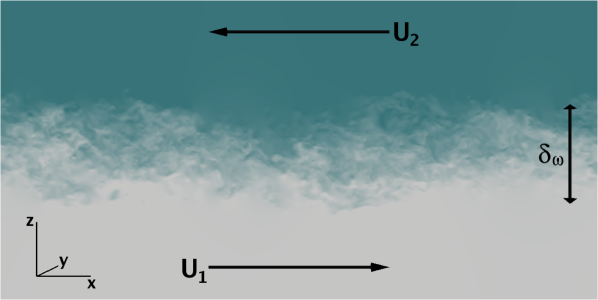
Figure 1: NFA simulation of a turbulent mixing layer. The illustration is an $x-z$ plane of instantaneous streamwise, $x$, velocity. Note the wide range in the scales of motion, which is typical of shear generated turbulence.

The first type of simulation used to validate NFA is a temporally evolving shear layer. An example of this type of flow is shown in Figure 1 to provide a visual reference to the amount of disorder these flows generate, and a reference to the problem setup.

A shear layer develops when two streams of fluid with different velocities are brought together. This type of flow is representative of many engineering and geophysical flows. The analysis of this type of flow is simplified because the statistical description of the flow reduces to a single dimension. It is often considered a canonical flow to study fundamental aspects of turbulence, and has been extensively studied both experimentally (Corcos and Sherman (1976), Bell and Mehta (1990) and Spencer and Jones (1971), amongst others) and numerically (Rogers and Moser (1994), Pantano and Sarkar (2002) and Brucker and Sarkar (2007), again amongst others). These detailed studies provide a rich database to compare with, and these comparisons serve to assess the ability of NFA to simulate highly turbulent flows.

Here, the velocity streams, $U_{1}$ and $U_{2}$, are of equal magnitude and opposite sign, with the velocity difference across the two streams being $\Delta U\equiv U_{1}-U_{2}$. The model flow evolves temporally in a domain that moves with the mean convective velocity $U_{C}=\left(U_{1}+U_{2}\right)/2=0$. The thickness of the mixed region grows in time and can be characterized by the vorticity thickness, $\delta_{\omega}(t)$ and then momentum thickness, $\delta_{\theta}(t)$, respectively defined as:

$$\delta_{\omega}(t)\equiv\frac{\Delta U}{\left(d\left<u\right>/dx_{3}\right)_{max}},$$ (38)

$$\delta_{\theta}(t)=\int^{\infty}_{-\infty}\left(\frac{1}{4}-\left<u_{1}\right>^{2}/\Delta U^{2}\right)dx_{3}.$$ (39)

In the preceding equations the $\left<\cdot\right>$ operator denotes an average over the $x_{1}-x_{2}$ plane, and fluctuations with respect to the mean are obtained by applying a Reynolds decomposition, $u_{i}=\left<u_{i}\right>+u^{\prime}_{i}$.

5.1.1 Initial Conditions

The initial conditions are constructed as a mean component plus a small random disturbance. The adjustment procedure of Dommermuth et al. (2002), in which the mean is held constant until the production reaches a steady value, is used. The adjustment time was $10\delta_{\omega,0}/\Delta U$. Figure 2 shows the $\left<u^{\prime}_{1}u^{\prime}_{3}\right>$ cross-correlation responsible for turbulent production. By $t=8$ the a constant value was reached, and at $t=10$ the mean was allowed to evolve. This type of adjustment procedure removes the arbitrary addition of “turbulent like” fluctuations, and allows for repeatable initial conditions.

The mean initial conditions are:

$$\left<u_{1}\right>=-\frac{\Delta U}{2}{\rm tanh}\left(\frac{2x_{3}}{\delta_{\omega,0}}\right),\\ \left<u_{2}\right>=\left<u_{3}\right>=\left<p\right>=0.$$ (40)

where $\delta_{\omega,0}=1$ and $\Delta U=1$.

The amplitude of the random fluctuations added to the mean velocity was $0.0165\Delta U$.

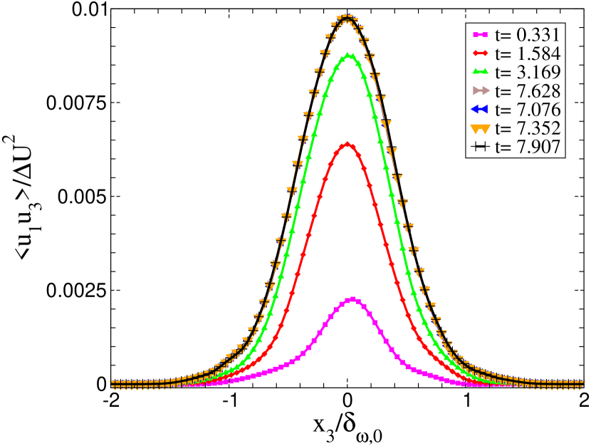
Figure 2: Reynolds shear stress responsible for turbulent production at several times during the adjustment phase.

The computational domain $[L_{1},L_{2},L_{3}]=[36.0,12.0,18.0]\delta_{\omega,0}$ was discritized with $[N_{1},N_{2},N_{3}]=[384,128,192]$ computational nodes. The time step was $\Delta t=0.001\delta_{\omega,0}/\Delta U$. Periodic boundary conditions were used in the stream-wise ($x,x_{1}$) and span-wise ($y,x_{2}$) direction for all variables. In the cross-stream direction ($z,x_{3}$), Dirichlet boundary conditions were used for the vertical velocity and Neumann boundary conditions were used for the other velocity components and pressure.

(a)
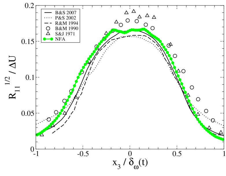
(b)
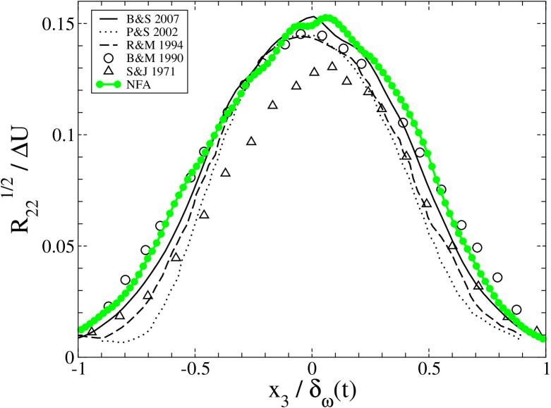
(c)

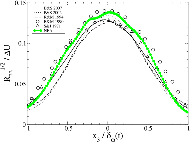
Figure 3: (a) Streamwise, (b) Spanwise, (c) Cross-stream $r.m.s.$ velocities. The abbreviations in the legend are as follows: B&S 2007 refers to the DNS of Brucker and Sarkar (2007), P&S 2002 refers to the DNS of Pantano and Sarkar (2002), R&M 1994 refers to the DNS of Rogers and Moser (1994), B&M 1990 refers to the experiments of Bell and Mehta (1990), and S&J 1971 refers to the experiments of Spencer and Jones (1971).

(a)

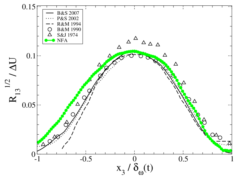
(b)

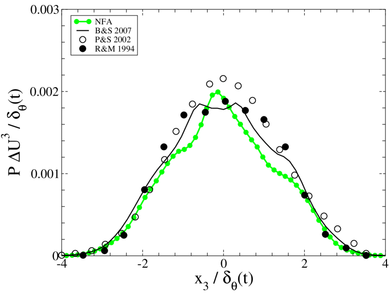
Figure 4: (a) Reynolds shear stress $\left<u^{\prime}_{1}u^{\prime}_{3}\right>$. (b) Turbulent production. References in legend as in Figure (3).

5.2 Shear Layer Turbulence

Figures 3(a)-(c) compare the Reynolds stresses, $R_{ij}=\left<u^{\prime}_{i}u^{\prime}_{j}\right>$ for $i=j$, obtained here with data from previous studies. The Reynolds stresses were evaluated by averaging the self-similar form at the following times: $\delta_{\omega,0}/Ut=$ 110, 120, and 130 $\delta_{\omega,0}/\Delta U$. The peak streamwise, transverse, and spanwise turbulent intensities, shown in Figures 3(a)-(c), $\sqrt{R_{11}}/\Delta U=0.17$, $\sqrt{R_{33}}/\Delta U=0.14$, and $\sqrt{R_{22}}/\Delta U=0.15$ agree well with previous DNS and experimental data. The experimental data shows a scatter of about $10\%$ with respect to the simulation data. The shape of the self-similar profiles also agrees well. Comparisons of the the Reynolds stresses, $R_{ij}=\left<u^{\prime}_{i}u^{\prime}_{j}\right>$ for $i\neq j$, and the production of turbulent kinetic energy defined as:

$$P\equiv-\left<u^{\prime}_{i}u^{\prime}_{j}\right>\frac{\partial\left<u_{i}\right>}{\partial x_{j}}=-\left<u^{\prime}_{1}u^{\prime}_{3}\right>\frac{\partial\left<u_{1}\right>}{\partial x_{3}}\;,$$ (41)

in the current simulations to that from an incompressible DNS (Rogers and Moser (1994),Brucker and Sarkar (2007) and compressible low Mach number DNS (Pantano and Sarkar (2002) are shown in Figure 4(a)-(b), respectively. The results from the current simulations agree well with previous DNS and laboratory data.

In summary, the turbulent shear layer simulations have been successfully bench marked against previous laboratory and DNS data, and show NFA’s ability to correctly capture the energetically important scales of turbulent motion without requiring explicit modeling.

6 Flow over a Sphere

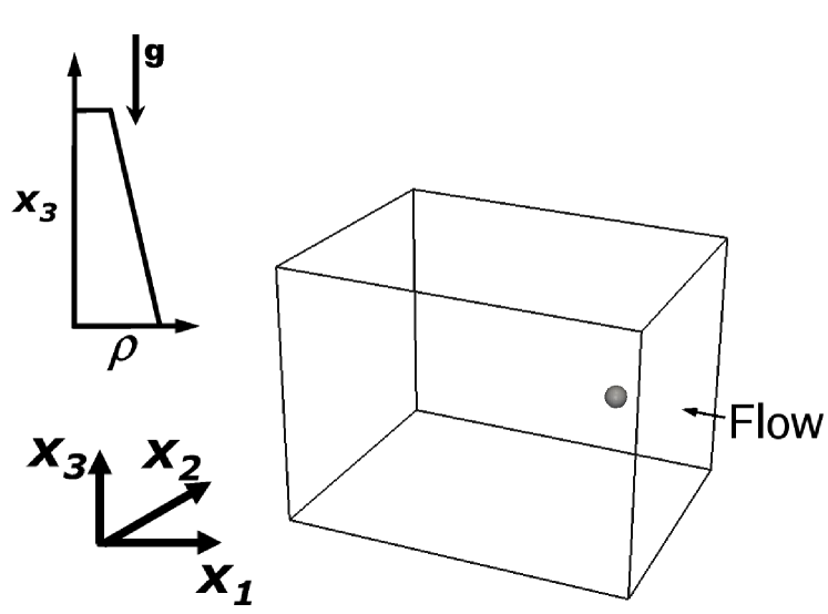
Figure 5: A schematic of the computational domain.

NFA simulations of flow over a sphere in uniform and stratified fluids are respectively discussed. The computational domain is shown schematically in Figure 5. The size of the computational domain $[L_{1},L_{2},L_{3}]$, the number of computational nodes $[N_{1},N_{2},N_{3}]$, the near body grid spacing, $\Delta x_{i}^{NB}$, the time step, $\Delta t$, the internal Froude number, $Fr$, and the near-body parameter $\beta$ are provided in Table 1 for all simulations subsequently discussed.

All of the simulations used In-flow and Out-flow boundary conditions in the stream-wise ($x_{1}$) direction, and Neumann boundary conditions in the span-wise ($x_{2}$) direction. In the cross-stream direction ($x_{3}$), Dirichlet boundary conditions are used for the vertical velocity, $u_{3}$, and Neumann boundary conditions are used for the other velocity components, pressure, and density.

In the NFA simulations the flow is accelerated from rest by multiplying the free-stream current with the following function:

$$f(t)=\left\{1-exp\left[-\left(t/T_{cur}\right)^{2}\right]\right\}.$$ (42)

$T_{cur}=0.5$ was used in all simulations.

Table 1: Parameters for all sphere simulations. Domain size, grid points, grid spacing near the body, time step, near body parameter, $\beta$. All normalized with the body diameter $D$ and free-stream velocity $U$. The internal Froude number, $Fr$, for each case is given by the case name. Cases labeled $FrX$ denote a domain used for runs at different Froude numbers.

Case	$L_{x}$	$L_{y}$	$L_{z}$	$N_{x}$	$N_{y}$	$N_{z}$	$\Delta t$	$\beta$	$\Delta x_{i}^{NB}$
$Fr1_{1}$	19	20	10	512	384	384	0.0025	0.67	0.03
$Fr1_{2}$	19	20	5	512	384	256	0.0020	0.33	0.03
$Fr4_{1}$	19	20	10	1024	768	768	0.00125	1.00	0.01
$Fr4_{2}$	19	20	5	512	384	256	0.002	0.33	0.03
$Fr{\infty}_{1}$	10	8	8	1024	768	768	0.001	1.00	0.008
$Fr{\infty}_{2}$	10	8	8	1024	768	768	0.001	0.00	0.008
$FrX^{C}$	12	6	6	384	256	256	0.005	0.67	0.03
$FrX^{M}$	12	12	12	384	384	384	0.005	0.67	0.03

6.1 Uniform fluid

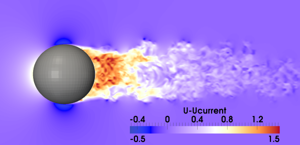
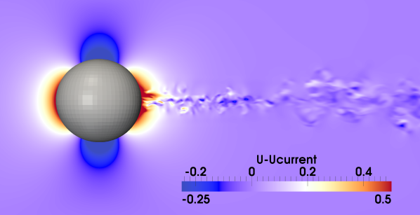
Figure 6: NFA simulations of unstratified flow over a sphere. The illustrations are of the instantaneous stream-wise velocity on the $x-z$ plane located at $y=0$. Top case $Fr\infty_{1}$ with $\beta=1$. Bottom case $Fr\infty_{2}$ with $\beta=0$.

Contours of the instantaneous streamwise velocity on the $x-z$ plane located at $y=0$ are shown in Figure 6 for cases $Fr\infty_{1}$ with $\beta=1$ (top) and $Fr\infty_{2}$ with $\beta=0$ (bottom). When $\beta=0$ the boundary conditions on the body are no-slip and no flow separation occurs. When $\beta=1$ the flow separates just shy $120\deg$, the value reported in Achenbach (1972). Here, a comparison of the drag coefficient to theory and experiments is used to assess the quality of the flow near the body. Since in the unstratified case the drag is determined by the fields in the immediate vicinity of the body it is an excellent metric for determing the quality of those fields.

The drag coefficient, is defined as:

$$C_{D}\equiv\frac{F_{D}}{1/2\rho_{0}U^{2}A_{P}}\;,$$ (43)

where $F_{D}$ is the drag force and $A_{P}$ is the project frontal area of the body.

The drag force on the body is calculated by integrating the normal pressure over the surface. Achenbach (1972) reports that the viscous contribution to the drag is $\sim 2\%$ of the total at $Re=5\times 10^{6}$, and hence the the total drag should be well approximated by the pressure drag at high-Re. The viscous contribution is not calculated.

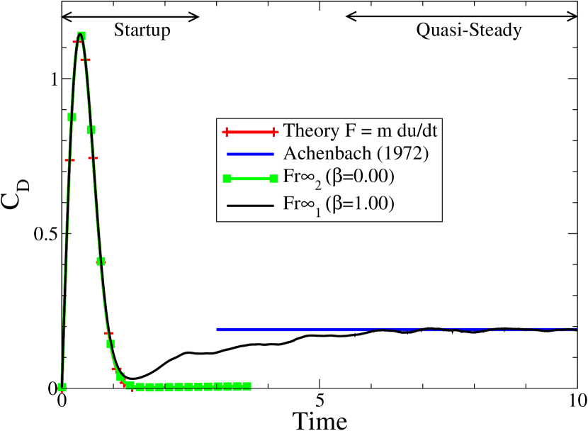
Figure 7: Drag coefficient for flow over a sphere at high-Reynolds number. The references in the legend are: Achenbach (1972) refers to the experiments of Achenbach (1972) while the theoretical prediction refers to equation 44.

The coefficient of drag for cases $Fr\infty_{1}$ with $\beta=1$ and $Fr\infty_{2}$ with $\beta=0$ are shown in Figure 7. As noted in the discussion of Figure 6 the free-slip boundary conditions, used in case $Fr\infty_{2}$, did not allow for flow separation and hence there was almost complete pressure recovery in the lee of the sphere and hence no drag. For case $Fr\infty_{1}$, in which separation occured at the correct location, the drag coefficient was $0.2$ the same value reported in the experiments of Achenbach (1972).

During the startup phase of the simulations, $f(t)$ is non-zero and there is an added mass component of the drag:

$$F_{D}^{AM}=mU\frac{df}{dt}$$ (44)

The drag due to the added mass is also shown in Figure 7, and the agreement between both simulations and the prediction is excellent.

6.2 Flow over a sphere in a stratified fluid

Having validated the drag on a sphere in the case without stratification, attention is now turned to the case with stratification. To proceed comparisons are made between existing theoretical and experimental data sets. The stratification of the fluid can cause body generated waves and significant drag at low Froude numbers ($\leq 1.5$), while at moderate Froude numbers ($1.5\geq Fr\leq 3$) the potential energy gained overcoming the poles of the sphere aids in pressure recovery in the lee and a small drag reduction.

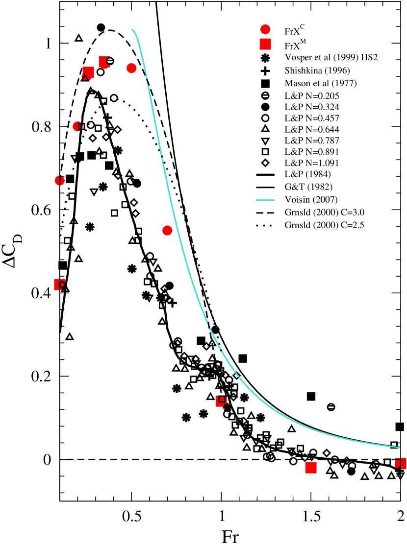
Figure 8: Change in the drag coefficient as a function of internal Froude number. In the legend, $FrX^{C}$ and $FrX^{M}$ denote cases with the coarse and medium resolutions reported in Table 1.

Following, Lofquist and Purtell (1984) the change in drag due to stratification, $\Delta C_{D}$, is defined as:

$$\Delta C_{D}(Fr)=C_{D}(Fr)-C_{D}\left(Fr\infty\right).$$ (45)

Figure 8 shows the change in the drag coefficient, $\Delta C_{D}$, as a function of the internal Froude number, $Fr=U/(2rN)$. NFA simulations at $Fr=0.1,0.2,0.25,0.35,0.5,0.75,1.0,1.5,2.0$ are compared with the theories of Greenslade (2000), Voisin (2007), and Gorodtsov and Teodorovich (1982) along with the experiments of Lofquist and Purtell (1984), Vosper et al. (1999), Shishkina (1996), and Mason (1977).

In summary, Figure 8 shows that NFA is able to predict correctly the change in drag for both low and moderate Froude numbers, and appears to correctly predict the transition from low to high Froude number regimes, which occurs between $Fr\approx 0.7$ and $Fr\approx 1.0$, although this prediction currently is based on only one computed data point.

7 INTERNAL WAVES

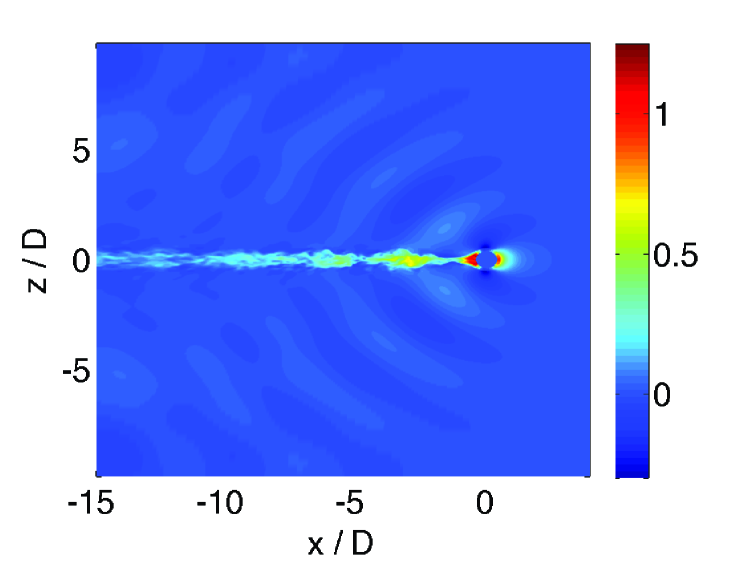
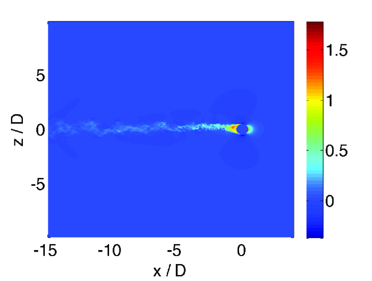
Figure 9: Along track vertical $(x,z)$ plane at $y=0$ of the numerical solutions at the wake center for $Fr=1$ (upper panel) and $Fr=4$ (lower panel). The plotted variable is $u/U$, the $x$-component of the velocity of the wavefield.

We now compare the internal waves computed by NFA for stratified flow over a sphere with the field predicted by linear wave theory, using an oscillating source distribution to parameterize the generation of the waves by the sphere and its wake, as discussed in The Fourier-Ray Model section. As this is a preliminary study, we consider flows for just two moderate Froude numbers, $Fr=1$ and $4$. The sphere is towed in the positive $x$ direction, and each plot shown below is either a horizontal $(x,y)$ cross section at a height of two sphere diameters ($z=2D$) above the centerplane of the sphere or a vertical $(x,z)$ plane through the wake centerline. The plots show the $x$ component $u$ of the wavefield velocity.

For the Fourier-ray calculations, the inverse Fourier transform (2) was approximated discretely on a wavenumber grid of 1024 by 512 in $k,l$, for $Fr=1$ and $Fr=4$. In addition to resolving the flow features, the extent of the wavenumber grid must be chosen to limit periodic wrap-around errors, which result from the discrete approximation of the inverse Fourier transform. For a single depth, the theoretical solution takes only a few seconds to calculate on a standard PC.

Figure 9 shows the horizontal velocity $u/U$ on a vertical plane through the wake centerline ($y=0$) for the two cases $Fr=1$ (top pane) and $Fr=4$ (bottom pane). The lower Froude number case shows a well-defined lee wave field as well as a weakly turbulent wake. The lee wave field is steady with respect to the sphere, but downstream of about $x/D=-5$ internal waves generated by the turbulent wake can be seen. For the higher Froude number, the lee waves are very weak and the turbulent wake is stronger and shows evidence of periodic fluctuations.

Figure 10 show results for the case of $Fr=1$. The numerical simulation result is shown in the top panel, and the linearized theory, with $\sigma=0$, in the lower panel. In this case the upper and lower boundaries of the simulations are sufficiently far away for there to be no reflections that would be seen in the domain shown in these figures. The two results are very close, with some small differences appearing downstream of $x/D=-5$ near $y=0$. At this relatively low Froude number the body-generated waves dominate over the wake-generated waves. It appears from these results that the proposed source representation of the sphere produces an accurate internal wave field, even though the source function we have used, (9), is most accurate for the representation of a solid sphere only in the limit of high Froude number. However, the discrepancies that are seen further downstream are due to weak internal waves generated by the wake turbulence that can be seen in figure 9. This effect is better visualized in figure 11, which is a plot of $u/U$ in the vertical plane located at $y=0$. Only the positive $z$ half of the plane is shown. In these plots the linear theory (lower panel) shows waves emanating only from the sphere, where as the numerical simulations clearly show waves emanating from the sphere and from locations downstream of the sphere.

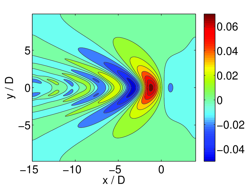
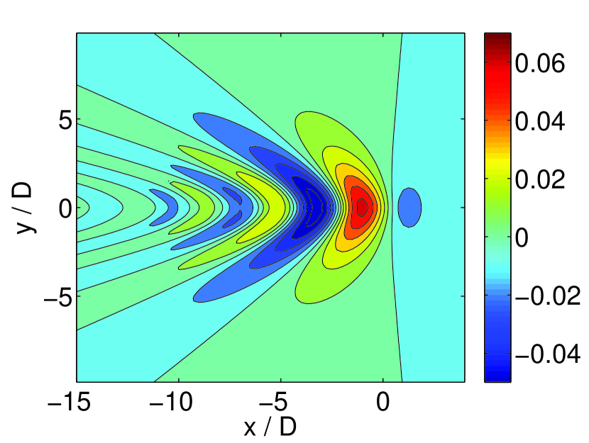
Figure 10: A comparison for $Fr=1$ from the numerical simulations (upper panel) and from linear theory (lower panel), on the $(x,y)$ plane located at $z=2D$. The plotted variable is $u/U$, the $x$-component of the velocity of the wavefield.

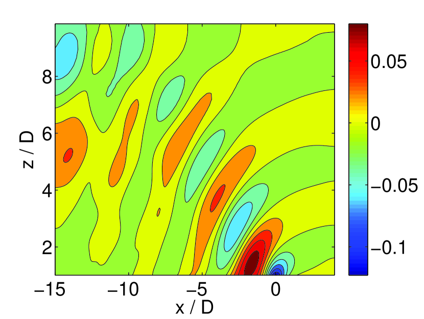
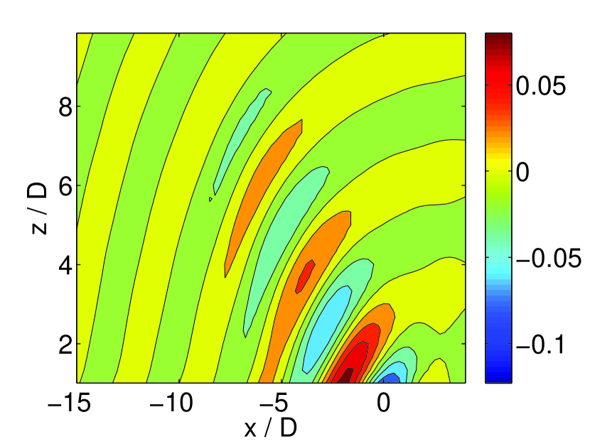
Figure 11: A comparison for $Fr=1$ from the numerical simulations (upper panel) and from linear theory (lower panel), for the positive$-y$ region of $(x,y)$ plane located at $z=2D$. The plotted variable is $u/U$, the $x$-component of the velocity of the wavefield.

Figure 12 show results for the case of $Fr=1$, now with the upper and lower boundaries at $z=\pm 5D$, which are close enough for the reflected waves to affect the observed wavefield. The numerical simulation result is shown in the top panel, and the linearized theory, with $\sigma=0$, in the lower panel. Again, the two results are very close, with some small differences appearing downstream of $x/D=-5$ near $y=0$, although the numerical simulations show some reflections from the sidewall boundaries. The linear theory was computed without sidewall boundaries. The discrepancies seen downstream and near the centerline are attributable to wake-generated waves, which are not accounted for in the linear theory.

Figures 13 and 14 show $u/U$ on a horizontal plane and a vertical plane, respectively, for $Fr=4$. Here the linear theory, with $\sigma=0$, is a poor representation of the solution, though it does give a reasonable prediction for the lateral extent of the wavefield. This is the Froude number regime in which wake-generated internal waves are expected to dominate over the body-generated waves. The wave amplitudes shown are quite small, and apparently significantly affected by the wake-generated waves. These results are very preliminary; we intend to continue the study by extending the numerical simulations farther downstream and comparing these results with the linear theory that includes combinations of nonzero source oscillation frequencies. The hope is that we will be able to determine the correct distribution of oscillation frequencies and oscillation amplitudes so that the linear theory will accurately reproduce the internal wave fields in these simulations.

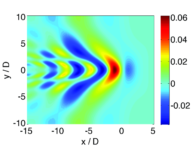
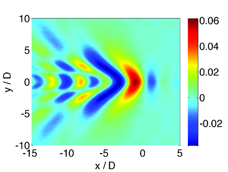
Figure 12: A comparison for $Fr=1$, with upper and lower horizontal boundaries located at $z=\pm 5D$, from the numerical simulations (upper panel) and from linear theory (lower panel). The plotted variable is $u/U$, the $x$-component of the velocity of the wavefield.

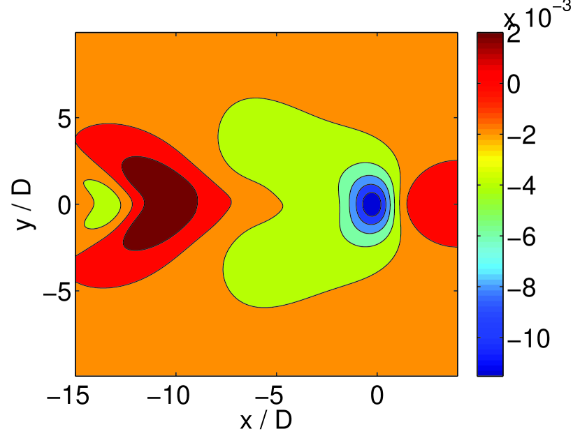
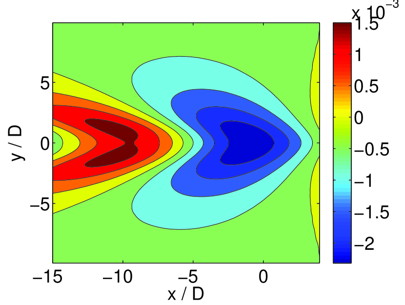
Figure 13: A comparison for $Fr=4$ from the numerical simulations (upper panel) with the linear theory (lower panel), on the $(x,y)$ plane located at $z=2D$. The plotted variable is $u/U$ on a horizontal plane at $z/D=2$.

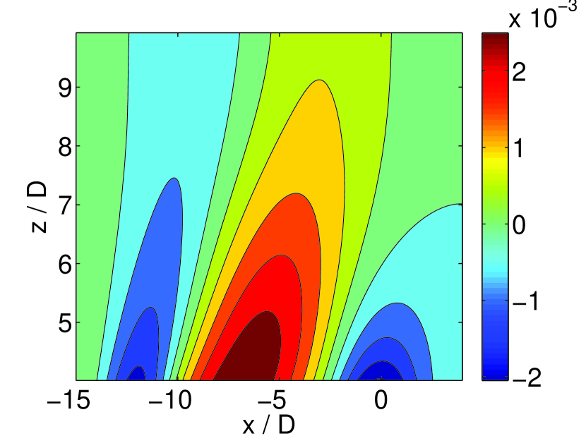
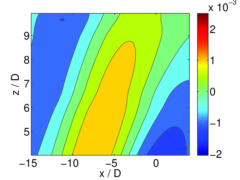
Figure 14: A comparison for $Fr=4$ from the numerical simulations (upper panel) with the linear theory (lower panel), for the positive$-z$ region of the $(x,z)$ plane located at $y=0$. The plotted variable is $u/U$.

8 CONCLUSIONS

In this paper, we have extended the capabilities of the numerical model NFA to high Reynolds number flows around obstacles in a stratified fluid. We have demonstrated that NFA (1) is capable of accurately reproducing the physics associated with highly turbulent flows; (2) is capable of accurately reproducing highly turbulent flows which separate due to the geometry of the body obstructing the flow; and (3) is capable of simulating stratified flows at low and high Froude numbers.

This work is another step in seeing how well ray theory can simulate the internal wavefield generated by stratified flow past an obstacle. In a previous paper, Rottman et al. (2004a) we compared ray theory with laboratory experimental results. In this paper we have begun a comparison of the ray simulation with the numerical model results for uniform background with reflecting upper and lower boundaries. The results show that the source distribution produces a very good representation of the internal wave field for low Froude numbers near unity where we would expect waves generated by the body itself to dominate. At higher Froude numbers, where the dominated wave generation is by the turbulent wake, the comparisons are not as good. This study will be continued in the future, now that NFA is available for these kinds of comparisons, to determine specifically what distribution of oscillating sources best models the wave generation by eddies in the wake.

9 Acknowledgements

This research was sponsored by Dr. Ron Joslin at the Office of Naval Research (contract number N00014-08-C-0508), Dr. Tom C. Fu at the Naval Surface Warfare Center, Carderock Division, and SAIC’s Research and Devlopment program. The numerical simulations were supported in part by a grant from the Department of Defense High Performance Computing Modernization Program (http://www.hpcmo.hpc.mil/). The numerical simulations were performed on the SGI Altix ICE 8200LX at the U.S. Army Engineering Research and Development Center.

Animated versions of the numerical simulations described here as well as many others are available online at: http://www.youtube.com/waveanimations

References

- (1)
- Achenbach (1972) Achenbach, E., “Experiments on the flow past spheres at very high reynolds number,” J. Fluid Mech., Vol. 54, no. 3, 1972, pp. 565–575.
- Bell and Mehta (1990) Bell, J. H. and Mehta, R. D., “Development of a two-stream mixing layer from tripped and untripped boundary layers.” AIAA J., Vol. 28, 1990, pp. 2034–2042.
- Broutman and Rottman (2004) Broutman, D. and Rottman, J., “A simplified fourier method for computing the internal wavefield generated by an oscillating source in a horizontally moving, depth-dependent background,” Phys. Fluids, Vol. 16, 2004, pp. 3682–3689.
- Broutman et al. (2003) Broutman, D., Rottman, J. W., and Eckermann, S. D., “A simplified fourier method nonhydrostatic mountain waves,” J. Atmos. Sci., Vol. 60, 2003, pp. 2686–2696.
- Brucker and Sarkar (2007) Brucker, K. A. and Sarkar, S., “Evolution of an initially turbulent stratified shear flow.” Phys. Fluids, Vol. 19, no. 10, 2007, p. 105,105.
- Corcos and Sherman (1976) Corcos, G. M. and Sherman, F. S., “Vorticity concentration and the dynamics of unstable free shear layers,” J. Fluid Mech., Vol. 73, 1976, pp. 241–264.
- Dommermuth et al. (1998) Dommermuth, D., Innis, G., Luth, T., Novikov, E., Schlageter, E., and Talcott, J., “Numerical simulation of bow waves,” Proceedings of the 22nd Symposium on Naval Hydrodynamics, Washington, D.C., 1998, pp. 508–521.
- Dommermuth et al. (2007) Dommermuth, D. G., O’Shea, T. T., Wyatt, D. C., Ratcliffe, T., Weymouth, G. D., Hendrickson, K. L., Yue, D. K. P., Sussman, M., Adams, P., and Valenciano, M., “An application of cartesian-grid and volume-of-fluid methods to numerical ship hydrodynamics,” Proceedings of the 9th International Symposium on Numerical Ship Hydrodynamics, held 5 – 8 August 2007 in Ann Arbor, Michigan, 2007.
- Dommermuth et al. (2002) Dommermuth, D. G., Rottman, J. W., Innis, G. E., and Novikov, E. A., “Numerical simulation of the wake of a towed sphere in a weakly stratified fluid,” J. Fluid Mech, Vol. 473, 2002, pp. 83–101.
- Dupont and Voisin (1996) Dupont, P. and Voisin, B., “Internal waves generated by a translating and oscillating sphere,” Dyn. Atmos. Oceans, Vol. 23, 1996, pp. 289–298.
- Gill (1982) Gill, A. E., Atmosphere-Ocean Dynamics, Academic Press, 1982.
- Gilreath and Brandt (1985) Gilreath, H. E. and Brandt, A., “Experiments on the generation of internal waves in a stratified fluid,” AIAA J., Vol. 23, 1985, pp. 693–700.
- Gorodtsov and Teodorovich (1982) Gorodtsov, V. A. and Teodorovich, E. V., “Study of internal waves in the case of rapid horizontal motion of cylinders and spheres,” Fluid Dynamics, Vol. 17, 1982, pp. 893–898.
- Gorostov and Teodorovich (1980) Gorostov, V. A. and Teodorovich, E. V., “On the generation of internal waves in the presence of uniform straight-line motion of local and nonlocal sources,” Izv. Atmos. Oceanic Phys., Vol. 16, 1980, pp. 699–704.
- Gorostov and Teodorovich (1981) Gorostov, V. A. and Teodorovich, E. V., “Two-dimensional problem for internal waves generated by moving singular sources,” Fluid Dynamics, Vol. 16, 1981, pp. 219–224.
- Gorostov and Teodorovich (1982) Gorostov, V. A. and Teodorovich, E. V., “Study of internal waves in the case of rapid horizontal motion of cylinders and spheres,” Fluid Dynamics, Vol. 17, 1982, pp. 893–898.
- Gorostov and Teodorovich (1983) Gorostov, V. A. and Teodorovich, E. V., “Radiation of internal waves by periodically moving sources,” Appl. Mech. Tech. Phys., Vol. 24, 1983, pp. 521–526.
- Greenslade (2000) Greenslade, M. D., “Drag on a sphere moving horizontally in a stratified fluid,” J. Fluid Mech., Vol. 418, 2000, pp. 339–350.
- Hardy (1949) Hardy, G. H., Divergent Series, Clarendon, 1949.
- Hoffman (2006a) Hoffman, J., “Adaptive simulation of the subcritical flow past a sphere.” J. Fluid Mech., Vol. 568, 2006a, pp. 77–88.
- Hoffman (2006b) Hoffman, J., “Simulation of turbulent flow past bluff bodies on coarse meshes using general galerkin methods: drag crisis and turbulent euler solutions.” Comput. Mech., Vol. 38, 2006b, pp. 390–402.
- John (2002) John, V., “Slip with friction and penetration with resistance boundary conditions for the navier-stokes equations - numerical tests and aspects of the implementation,” J. Comp. Appl. Math., Vol. 147, 2002, pp. 287–300.
- Knupp and Steinberg (1993) Knupp, P. M. and Steinberg, S., Fundamentals of grid generation, CRC Press, 1993.
- Leonard (1997) Leonard, B., “Bounded higher-order upwind multidimensional finite-volume convection-diffusion algorithms,” W. Minkowycz and E. Sparrow, eds., Advances in Numerical Heat Transfer, Taylor and Francis, Washington, D.C., 1997, pp. 1–57.
- Lighthill (1978) Lighthill, J., Waves in Fluids, Cambridge University Press, 1978.
- Lofquist and Purtell (1984) Lofquist, K. E. B. and Purtell, P., “Drag on a sphere moving horizontally through a stratified liquid,” J. Fluid Mech., Vol. 148, 1984, pp. 271–284.
- Mason (1977) Mason, P. J., “Forces on spheres moving horizontally in rotating stratified fluid,” Astrophys. Fluid Dyn., Vol. 8, 1977, pp. 137–154.
- Meyer et al. (2010a) Meyer, M., Devesa, A., Hickel, S., Hu, X. Y., and Adams, N. A., “A conservative immersed interface method for large-eddy simulation of incompressible flows,” J. Comput. Phys., Vol. in press.
- Meyer et al. (2010b) Meyer, M., Hickel, S., and Adams, N. A., “Assessment of implicit large-eddy simulation with a conservative immersed interface method for turbulent cylinder flow,” Int. J. Heat Fluid Flow, Vol. in press.
- Miles (1971) Miles, J. W., “Internal waves generated by a horizontally moving source,” Geophys. Astrophys. Fluid Dyn., Vol. 2, 1971, pp. 63–87.
- O’Shea et al. (2008) O’Shea, T. T., Brucker, K. A., Dommermuth, D. G., and Wyatt, D. C., “A numerical formulation for simulating free-surface hydrodynamics,” Proceedings of the 27th Symposium on Naval Hydrodynamics, Seoul, Korea, 2008.
- Pantano and Sarkar (2002) Pantano, C. and Sarkar, S., “A study of compressibility effects in the high-speed turbulent shear layer using direct simulation,” J. Fluid Mech., Vol. 451, 2002, pp. 329–371.
- Robey (1997) Robey, H. F., “The generation of internal waves by a towed sphere and its wake in a thermocline,” Phys. Fluids, Vol. 9, 1997, pp. 3353–3367.
- Rogers and Moser (1994) Rogers, M. M. and Moser, R. D., “Direct simulation of a self-similar turbulent mixing layer.” Phys. Fluids, Vol. 6, 1994, pp. 903–923.
- Rottman and Broutman (2008) Rottman, J. W. and Broutman, D., “Practical implementation of two-turning point theory for modeling internal wave propagation in a realistic ocean,” Proceedings of the 27th International Symposium on Naval Hydrodynamics, held 5 – 10 October 2008 in Seoul, Korea, 2008.
- Rottman et al. (2006) Rottman, J. W., Broutman, D., Spedding, G., and Diamessis, P., “A model for the internal wavefield produced by a submarine and its wake in the littoral ocean,” Proceedings of the 26th International Symposium on Naval Hydrodynamics, held 17 – 22 September 2006 in Rome, Italy, 2006.
- Rottman et al. (2004a) Rottman, J. W., Broutman, D., Spedding, G., and Meunier, P., “The internal wave field generated by the body and wake of a horizontally moving sphere in a stratified fluid,” Proceedings of the 15th Australasian Fluid Mechanics Conference, held 13 – 17 December 2004 in Sydney, Australia, 2004a.
- Rottman et al. (2004b) Rottman, J. W., Broutman, D., Spedding, G., and Meunier, P., “Internal wave generation by a horizontally moving sphere at low Froude number,” Proceedings of the 25th International Symposium on Naval Hydrodynamics, held 8 – 13 August 2004 in St. John’s, Newfoundland and Labrador, Canada, 2004b.
- Shishkina (1996) Shishkina, O. D., “Comparisons of the drag coefficients of bodies moving in liquids with various stratification profiles,” Fluid Dynamics, Vol. 31, 1996, pp. 484–489.
- Spencer and Jones (1971) Spencer, B. W. and Jones, B. G., “Statistical investigation of pressure and velocity fields in the turbulent two-stream mixing layer.” AIAA Paper, Vol. 71-613, 1971, pp. 2034–2042.
- Sussman and Dommermuth (2001) Sussman, M. and Dommermuth, D., “The numerical simulation of ship waves using cartesian-grid methods,” Proceedings of the 23rd Symposium on Naval Ship Hydrodynamics, Nantes, France, 2001, pp. 762–779.
- Voisin (1994) Voisin, B., “Internal wave generation in uniformly stratified fluids. part 2. moving point sources,” J. Fluid Mech., Vol. 261, 1994, pp. 333–374.
- Voisin (2007) Voisin, B., “Lee waves from a sphere in a stratified flow,” J. Fluid Mech., Vol. 574, 2007, pp. 273–315.
- Vosper et al. (1999) Vosper, S. B., Castero, I. P., Snyder, W. H., and Mobbs, S. D., “Experimental study of strongly stratified flows past three-dimensional orography,” J. Fluid Mech., Vol. 390, 1999, pp. 223–239.