Application of a Solar Wind Model Driven by Turbulence Dissipation to a 2D Magnetic Field Configuration

Abstract

Although it is widely accepted that photospheric motions provide the energy source and that the magnetic field must play a key role in the process, the detailed mechanisms responsible for heating the Sun’s corona and accelerating the solar wind are still not fully understood. Cranmer et al. (2007) developed a sophisticated, 1D, time-steady model of the solar wind with turbulence dissipation. By varying the coronal magnetic field, they obtain, for a single choice of wave properties, a realistic range of slow and fast wind conditions with a sharp latitudinal transition between the two streams. Using a 1D, time-dependent model of the solar wind of Lionello et al. (2014), which incorporates turbulent dissipation of Alfvén waves to provide heating and acceleration of the plasma, we have explored a similar configuration, obtaining qualitatively equivalent results. However, our calculations suggest that the rapid transition between slow and fast wind suggested by this 1D model may be disrupted in multidimensional MHD simulations by the requirement of transverse force balance.

1 INTRODUCTION

Although the physical processes responsible for heating the solar corona and accelerating the solar wind have not been unambiguously identified, it is thought that the interaction of the magnetic field with random motions on the photospheric surface may play a crucial role. Since measurements of wind speeds in fast streams indicate that the deposition of heat occurs over extended length scales (Withbroe & Noyes, 1977; Holzer & Leer, 1980; Withbroe, 1988), one-dimensional (1D) models of the solar wind in the past have included parametric heating forms involving exponential functions decaying with the distance above the Sun’s surface (Hammer, 1982a, b; Withbroe, 1988; Hansteen & Leer, 1995; Habbal et al., 1995; Hansteen et al., 1997). More sophisticated treatments have derived acceleration and heating rates for the solar wind based on the dissipation of long-period, large-scale, broadband fluctuations (Coleman, 1968; Belcher & Davis, 1971; Hollweg, 1986; Hollweg & Johnson, 1988; Velli, 1994; Matthaeus et al., 1999; Verdini & Velli, 2007; Zank et al., 2012).

In the context of MHD models of the solar coronal and inner heliosphere, because of the very large temporal and spatial ranges that are involved in the dynamics, it is complicated to connect the large-scale heating formulation for the heating of the plasma and the acceleration of the wind with the underlying physical mechanisms. During the past years and with different levels of self-consistency, mechanisms for turbulent dissipation have been integrated into 1D models of the solar wind (Suzuki & Inutsuka, 2005; Cranmer & van Ballegooijen, 2005; Cranmer et al., 2007; Cranmer, 2010; Verdini et al., 2010; Chandran et al., 2011; Lionello et al., 2014). Formulas for turbulence dissipation are also increasingly replacing empirical heating functions in three-dimensional (3D) MHD models such as those of Lionello et al. (2009) or Downs et al. (2010). Since these 3D models would have to resolve both the temporal scales related to dissipation in the solar corona (of the order of milliseconds) and those related to large structures in the solar wind (many days), this integration represents a formidable challenge. Proton heating through Kolmogorov dissipation in regions of open magnetic field, together with Alfvén waves acceleration of the solar wind, was implemented in the model of van der Holst et al. (2010). The large-scale MHD model of the heliosphere of Usmanov et al. (2011) includes, for the region where the solar wind is superalfvénic and supersonic, a formulation for the transport and dissipation of turbulence energy. A phenomenological description of nonlinear interactions, which are ascribed to wave reflection caused by chromospheric and coronal density gradients, is present in the model of Lionello et al. (2013), including the outward propagation Alfvénic turbulence in the solar wind. Sokolov et al. (2013) implemented an Alfvénic turbulent transport and dissipation mechanism, which both heats the coronal plasma and accelerates the solar wind (further details are presented in van der Holst et al., 2014). Finally, Matsumoto & Suzuki (2012, 2014) proposed an integrated, 2.5D model that connects the photosphere and the inner heliosphere. The model inputs only torsional Alfvén waves at the coronal base, allowing coupling with both parallel (sound) and transverse magnetoacoustic modes. Reflection is self-consistently included. Though both polarizations transverse to the radial are included, there is only one transverse direction so that a purely incompressible transverse cascade in the spirit of Reduced Magnetohydrodynamics (RMHD) does not occur. Rather Matsumoto and Suzuki see complex compressive interactions between the average radial wind and the fluctuations, including parametric decay. In the same spirit of the works of Matsumoto and Suzuki are the 2D simulations of Ofman & Davila (1998) and Ofman (2005). On the other hand, it is the features of such a cascade that our simpler 1D models attempt to capture phenomenologically (Lionello et al., 2014).

Notwithstanding the appeal of multidimensional models, 1D simulations still play a crucial role, since they can reach a level of sophistication in the physical model and of resolution in the calculation that are not otherwise achievable. They also constitute fundamental tests to which the results of multidimensional models must be reconciled. However, there is also a risk of extending the validity of results obtained through 1D simulations to more realistic configurations in which they may not necessarily apply.

Cranmer et al. (2007) developed a sophisticated, 1D, time-steady model of the solar wind, from the photosphere to the inner heliosphere. Their model uses sound and Alfvén waves for flow acceleration and turbulence dissipation for plasma heating. By varying the coronal magnetic field (based on the 2D, force-free, analytic model of Banaszkiewicz et al., 1998), they obtain, for a single choice of wave amplitude and correlation length at the base, a realistic latitudinal range of slow and fast wind conditions, as measured by the Ulysses spacecraft (e.g. Bame et al., 1992). Hence, the characteristics of the solar wind solution along each open flux tube are solely determined by the properties of the magnetic field, in agreement with the prescription of empirical models, such WSA (Wang & Sheeley, 1990; Arge et al., 2004), or empirically-driven, such as Riley et al. (2001).

Using the 1D, time-dependent, solar wind model of Lionello et al. (2014), we explore an almost identical magnetic configuration, calculating solar wind solutions along selected field lines, and obtaining results that confirm the results of Cranmer et al. (2007). However, by examining the pressure gradients between neighboring flux tubes, we suggest that observed latitudinally sharp transitions between slow and fast flows, obtained with a single choice of turbulence parameters in the 1D models, may actually be smoothed out in multidimensional calculations.

This paper is organized as follows: in Sec. 2 we present the characteristics of our model, comparing similarities and differences with that of Cranmer et al. (2007). In Sec. 3 we present our solutions and show in what sense they confirm the results of Cranmer et al. (2007) and in what sense they question them. Our conclusions follow.

2 MODEL DESCRIPTION

Our 1D model of the solar wind is based on the treatment of turbulence dissipation and wave pressure acceleration presented in Verdini et al. (2010). As described in more details in Lionello et al. (2014), the model solves along an open magnetic field line the following set of time-dependent, 1D HD equations:

$$\frac{\partial\rho}{\partial t} = -\frac{1}{A}\frac{\partial}{\partial s}\left(AU\rho\right),$$ (1)

$$\rho\frac{\partial U}{\partial t} = -\rho U\frac{\partial U}{\partial s}-\frac{\partial}{\partial s}(p+p_{w})+g_{s}\rho+\mathsf{R}_{s}+\frac{1}{s^{2}}\frac{\partial}{\partial s}\left(s^{2}\nu\rho\frac{\partial U}{\partial s}\right),$$ (2)

$$\frac{\partial T}{\partial t} = -U\frac{\partial T}{\partial s}-(\gamma-1)\left(T{\frac{1}{A}\frac{\partial}{\partial s}A}U-\frac{m_{p}}{2k\rho}\left({\frac{1}{A}\frac{\partial}{\partial s}A}q-n_{e}n_{p}{Q(T)}+{H}\right)\right).$$ (3)

$$\frac{\partial z_{\pm}}{\partial t} = -[U\pm V_{a}]\frac{\partial z_{\pm}}{\partial s}+R_{1}^{\pm}z_{\pm}+R_{2}^{\pm}z_{\mp}-\frac{|z_{\mp}|z_{\pm}}{2\lambda_{\odot}\sqrt{A/A_{\odot}}},$$ (4)

$$R_{1}^{\pm} = -\frac{1}{2}[U\mp V_{a}]\left(\frac{\partial\log V_{a}}{\partial s}+\frac{\partial\log A}{\partial s}\right),$$ (5)

$$R_{2}^{\pm} = \frac{1}{2}[U\mp V_{a}]\frac{\partial\log V_{a}}{\partial s},$$ (6)

$$H = \rho\frac{|z_{-}|z_{+}^{2}+|z_{+}|z_{-}^{2}}{4\lambda_{\odot}\sqrt{A/A_{\odot}}},$$ (7)

$$p = 2nkT$$ (8)

$$p_{w} = \frac{1}{2}\rho\frac{(z_{-}-z_{+})^{2}}{8},$$ (9)

$$\mathsf{R}_{s} = \rho z_{+}z_{-}\frac{\partial\log A}{\partial s}.$$ (10)

With $s\geq R_{\odot}$ we indicate the distance along a magnetic field line, which is generally different from the radial coordinate $r$; $p$, $T$, $U$, and $\rho$, are the plasma pressure, temperature, velocity, and density. The number density, $n$, is assumed to be equal for protons and electrons. $k$ is Boltzmann constant. $g_{s}=g_{0}R_{\sun}^{2}\mathbf{\hat{b}\cdot\hat{r}}/r^{2}$ is the gravitational acceleration parallel to the magnetic field line ($\mathbf{\hat{b}}$). The kinematic viscosity is $\nu$. Along the field line, we call $A(s)=1/B(s)$ the area factor, which corresponds to the inverse of the magnetic field magnitude $B(s)$. The field aligned component of the vector divergence of the MHD Reynolds stress, $\mathbf{R}=(\delta\mathbf{b}\delta\mathbf{b}/4\pi-\rho\delta\mathbf{u}\delta\mathbf{u})$, is $R_{\mathsf{s}}$. $\delta\mathbf{u}$ and $\delta\mathbf{b}$ are respectively the fluctuations of the velocity $\mathbf{u}=U(s)\mathbf{\hat{b}}+\delta\mathbf{u}$ and of the magnetic field, $\mathbf{B}=B(s)\mathbf{\hat{b}}+\delta\mathbf{b}$, with $\mathbf{\hat{b}}\cdot\delta\mathbf{b}=0=\mathbf{\hat{b}}\cdot\delta\mathbf{u}$. $p_{w}={\delta\mathbf{b}^{2}}/{8\pi}$ is the wave pressure. In Eq. (3), the polytropic index is $\gamma=5/3$. The radiation loss function $Q(T)$ is as in Athay (1986). $n_{p}$ and $n_{e}$ are respectively the proton and electron number densities (which are equal for a hydrogen plasma). For the heat flux $q$, according to the radial distance, either a collisional (Spitzer’s law) or collisionless form (Hollweg, 1978) is employed. At a distance of $10R_{\odot}$ from the Sun, a smooth transition between the two forms occurs (Mikić et al., 1999). In Eq. (4), the Elsasser variables $\mathbf{z}_{\pm}=\delta\mathbf{u}\mp\delta\mathbf{b}/\sqrt{4\pi\rho}$ (Dmitruk et al., 2001) are advanced. $\mathbf{z}_{+}$ represents an outward propagating perturbation along a radially outward magnetic field line, while $\mathbf{z}_{-}$ is directed inwardly. The actual direction of $\mathbf{z}_{\pm}$ is assumed to be unimportant, provided that it is in the plane perpendicular to $\mathbf{\hat{b}}$ and that only low-frequency perturbations are relevant for the heating and acceleration of the plasma. Hence, we treat $z_{\pm}$ as scalars. The Alfvén speed along the field line is $V_{a}(s)=B/\sqrt{4\pi\rho}$. With $R_{1}^{\pm}$ and $R_{2}^{\pm}$ respectively, we indicate the WKB and reflection terms, which are related to the large scale gradients. $\lambda_{\odot}$ is the turbulence correlation scale at the solar surface. Thus the heating function $H$ (de Karman & Howarth, 1938; Matthaeus et al., 2004), $p_{w}$ and $\mathrm{R}_{s}$ (Usmanov et al., 2011, 2012) can all be expressed in terms of $z_{\pm}$. At the lower boundary, since the solar wind is subsonic, we are allowed to specify temperature and density, but the velocity must be determined by solving the 1D gas characteristic equations. Since the upper boundary is placed beyond all critical points, the characteristic equations are used for all variables. The amplitude of the outward-propagating (from the Sun) wave is imposed in the $z_{\pm}$ equations.

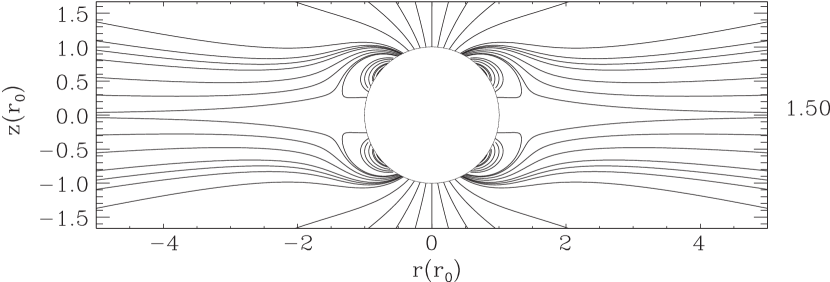
Figure 1: Magnetic field in the analytic model of Banaszkiewicz et al. (1998) for $Q=1.5$: we solve Eqs. (1-4) along selected field lines. Adapted from Fig. 2 of Banaszkiewicz et al. (1998).

For the present investigation, we express the area expansion factor $A(s)$ and the gravitational factor $g(s)$ along selected magnetic field lines calculated using the analytic model of Banaszkiewicz et al. (1998). This reproduces the characteristics of the magnetic field of the solar corona and interplanetary space during solar minimum by combining a dipole, a quadrupole, and a current sheet (Fig. 1). The magnetic field becomes basically radial at large distances from the Sun. We use the choice parameters that makes the last closed field line intersect the Sun at 60 degrees latitude and $B_{r}\sim 3.1~{}\mathrm{nT}$ at 1 AU ($K=1$, $M=1.789$, $a_{1}=1.538$, and $Q=1.5$ in Eqs.(1-2) in Banaszkiewicz et al., 1998).

The model of Cranmer et al. (2007) solves a set of equations equivalent to Eqs. (1-4) for mass, momentum, and energy conservation. However, it incorporates a more sophisticated treatment of the physics, which includes a number of features absent in our model, such as a photosphere, treatment of neutral hydrogen, and heating of the chromosphere through dissipation of a spectrum of sound waves. Moreover, the heating and acceleration of the solar wind through turbulence dissipation of Alfvén waves, which is also present in our model in the low-frequency limit, includes a broad series of frequencies. The solution methods employed in the two models are also different: while we use a time-dependent scheme, Cranmer et al. (2007) rely on an iteration and relaxation method. Since Cranmer et al. set the lower boundary in the photosphere, at low heights they modify the coronal magnetic field solution of Banaszkiewicz et al. (1998) according to the model of Cranmer & van Ballegooijen (2005).

3 RESULTS

Figure 2: Latitudinal dependence at 1AU of 1D solutions that were calculated along field lines of the magnetic field model of Banaszkiewicz et al. (1998) traced inward from 1AU: (a) wind speed; (b) number density; (c) temperature; (d) gas pressure. Each solution is marked with a cross.

We solve Eqs. (1-4) to obtain steady-state solar wind solutions along selected field lines of the force-free field of Banaszkiewicz et al. (1998). In all the solutions we use the same boundary conditions at the base of the domain, namely $n_{0}=2\times 10^{12}~{}\mathrm{cm^{-3}}$ and $T_{0}=20{,}000~{}\mathrm{K}$, to include the transition region and upper chromosphere in the calculation. A description of these boundary conditions at the base of the chromosphere is found in Mok et al. (2005) and Mikić et al. (2013). We likewise employ a technique to broaden artificially the transition region, while maintaining accuracy in the corona (Lionello et al., 2009). We have used a single combination of values $z_{+}^{\odot}=54~{}\mathrm{km/s}$ and $\lambda_{\odot}=0.02~{}R_{\odot}$ for Eq. (4), which, according to Lionello et al. (2014), is consistent with a fast stream solution. These values can be compared with those found in the model of Cranmer & van Ballegooijen (2005). Since the magnitude of the magnetic field of Banaszkiewicz et al. (1998) varies at the footpoints of open field lines between 11.8 and 7.7 G from pole to streamer, then, according to Eq. (51) of Cranmer & van Ballegooijen (2005), our correlation length $\lambda_{\odot}$ would be of the order of a network flux bundle. Furthermore, if we compare Figs. 3 and 11 of Cranmer & van Ballegooijen (2005), we find a that, at a height for which their magnetic field strength is the same as in our model, their magnitude of the Elsasser variables roughly agrees with ours, being between 50 and 60 km/s. A nonuniform mesh is employed with 631 points and $\Delta s$ ranging from $2.7\times 10^{-4}~{}R_{\odot}$ at the solar surface to $7.6~{}R_{\odot}$ at 1 AU. To damp unresolved scales below grid resolution, we add a small kinematic viscosity, such that the ratio of the associated dissipation time with the propagation time of Alfvén waves is $\tau_{\nu}/\tau_{A}=5000$ (Lionello et al., 2009).

3.1 Presentation

We have first explored the behavior of our model to see whether the observed dichotomy at 1 AU between the fast, rarefied polar and the slow, denser equatorial streams (e.g., Bame et al., 1992) could be reproduced with a single choice of turbulence parameters. Figure 2 shows the latitudinal dependence at 1AU of wind speed (2a), number density (2b), temperature (2c), and pressure (2d). Each point, marked with a cross, represents a value obtained with a 1D solution calculated along magnetic field lines traced inward from 1AU. We notice that the wind speed transitions from a fast polar stream to a slow equatorial as we move towards the current sheet. On the other hand, the number density of the plasma increases almost one order of magnitude close to the current sheet. Although the temperature decreases at lower latitudes, behaving similarly to the wind speed, the gas pressure turns out almost $80\%$ higher at $\pm 15^{\circ}$ around the current sheet. This result may be compared with Fig. 12 of Cranmer et al. (2007).

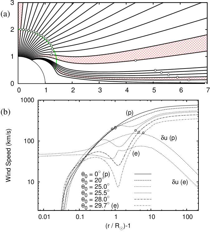
Figure 3: (a) Magnetic field lines from the model of Banaszkiewicz et al. (1998). The position of the critical points for sound waves for the 1D wind solutions calculated along them is indicated with circles. The green curve is drawn at a distance of 1 $R_{\sun}$ along of the field lines: the plasma pressure along the curve is plotted in Fig. 4a. The red filling between pairs of field lines indicates that the acceleration perpendicular to $\mathbf{\hat{b}}$ is plotted in Fig. 4b. (b) Wind speed calculated along several flux tubes prescribed with the same model. The speed is given as a function of the distance along the field line. The field lines originate from the solar surface at colatitudes varying between 0, polar field line, indicated with (p), and 29.7, field line that goes close to the equator, indicated with (e). The circles show where the wind becomes supersonic. The speeds of the perturbation, $\delta u$, for the (e) and (p) solutions are also shown.

Then we have considered how the solar wind speed varies along open magnetic flux tubes corresponding to the fast and the slow streams. Figure 3, which can be compared with Fig. 11 of Cranmer et al. (2007), shows the position of the sonic points and the speed of the solar wind calculated along several magnetic field lines. For each field line, the colatitude of the foot-point at the solar surface is indicated. The polar field line (p) originates from the pole; the equatorial field line (e) is the last open field line, since field lines with higher colatitude are closed. We also show the value of the turbulent velocity perturbation for the polar and equatorial field lines. The wind calculated along the polar field line as well as neighboring lines becomes rapidly supersonic at a length of less than $1~{}R_{\odot}$. Then there is a rapid transition between 25^∘ and $25.5^{\circ}$ colatitude, with the sonic point moving outwards and a deceleration zone appearing in its place. This zone becomes increasingly more pronounced as the foot-point is set at higher colatitudes. In agreement with what is shown in Fig. 2a, the final speed for solutions computed on magnetic field lines closer to the equator is considerably smaller.

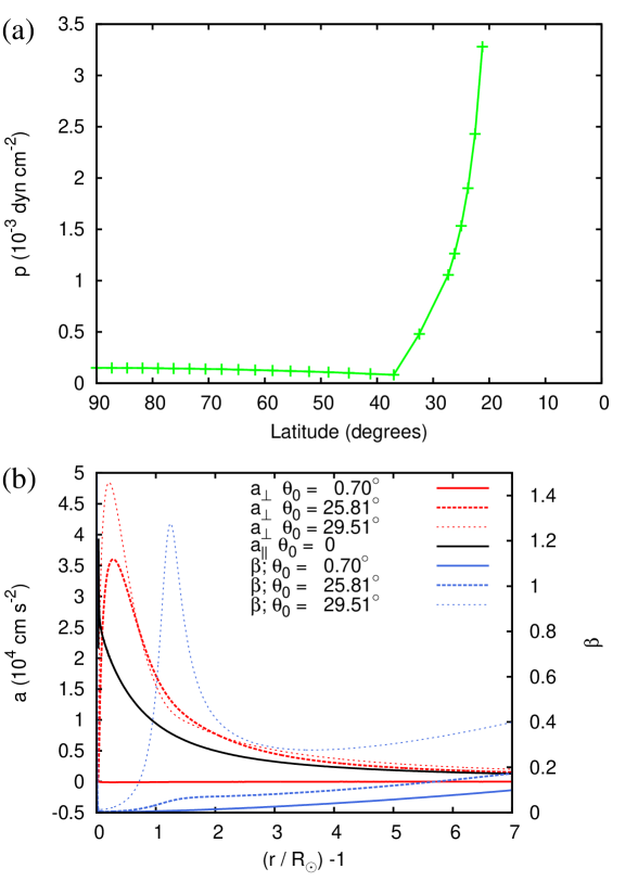
Figure 4: (a) The plasma pressure obtained from the 1D solar wind solutions and evaluated along the green curve shown in Fig. 3a. Each solution is marked with a cross. (b) In red: acceleration mainly due to pressure gradients perpendicular to $\mathbf{\hat{b}}$, obtained by differencing the pressure between two 1D solar wind solutions, calculated along magnetic field lines with colatitudes around $0.70^{\circ}$, $25.81^{\circ}$, and $29.51^{\circ}$ respectively. The pairs of magnetic field lines are shown in red in Fig. 3a. The contribution due to the centrifugal force, although it is included, is minimal. The acceleration is directed towards higher latitudes. In blue: the corresponding plasma $\beta$ at the same positions. In black: acceleration due to the pressure gradient along the magnetic field for the polar solution.

Figure 4a shows the pressure obtained with the 1D solutions and evaluated along the green curve of Fig. 3a, which is drawn at a distance of 1 $R_{\sun}$ along the field lines. Comparing with Fig. 3b, we notice that the pressure increases considerably as we move towards the equator, where, as predicted by Bernoulli’s principle (Bernoulli 1738, p. 231, or, for a more recent formulation, Lamb 1975, p. 20), a velocity stagnation point is present.

Since both Fig. 2 and Fig. 3 indicate a rapid latitudinal transition between the fast and the slow wind, we have calculated the acceleration perpendicular to the magnetic field, to determine whether the force-free magnetic field of Banaszkiewicz et al. (1998) would be capable of accommodating such gradients without considerable deviation from the analytic form. We selected three pairs of magnetic field lines, indicated with a red pattern in Fig. 3a, and for each calculated the quantity

$$a_{\perp}=\frac{1}{\rho}\frac{\Delta p}{\Delta l}+\frac{U^{2}}{R_{c}},$$ (11)

where $\Delta l$ is the distance perpendicular to the magnetic field and $R_{c}$ is the local radius of curvature. In the present cases, the first term on the right hand side of Eq. (11) dominates everywhere over the second. For the three pairs of magnetic field lines, we plot $a_{\perp}$ in red in Fig. 4b. The acceleration is directed from the current sheet towards the North Pole. The magnitudes of the perpendicular acceleration are not negligible, since they are comparable with the values of the acceleration $a_{\parallel}$ due to the parallel pressure gradient computed along the polar field line, which is shown in black in Fig. 4b. For the three examples, we also show in blue the plasma $\beta=4\pi p/B^{2}$. While $\beta$ is very small at high latitudes, it increases considerably as we move towards the current sheet, close to which it becomes larger than one. It follows that for field lines with footpoints at larger colatitudes a strong pressure gradient is expected to build. There is evidence in the literature that this would cause a restructuring of the magnetic field. For example, in the pioneering work of Pneuman & Kopp (1971), an isothermal model of the corona is calculated by imposing the equilibrium of forces normal to the magnetic field. More recently, Vásquez et al. (2003) used an iterative, 2D model of the solar corona with anisotropic gas pressure and found that the build up of perpendicular pressure gradients causes a reconfiguration of the magnetic field. Moreover, the presence of a stagnation point near the streamer cusp, in combination with the effects of plasma $\beta$ being of order 1 at the cusp, was studied by Suess & Nerney (2002) and Nerney & Suess (2005). Hence, in order to balance these normal gradients in a self-consistent MHD calculation, the equilibrium magnetic field must change. Since large variations of the equilibrium field are necessary to balance the pressure gradients, the solar wind solutions are also expected to change.

3.2 Discussion

Our results and those of Cranmer et al. (2007), in spite of quantitative differences, are in general qualitative agreement. The fact that our choice of turbulent parameters is different should not be surprising. For Cranmer et al. (2007) include the photosphere in their model and specify their boundary values at a lower height than we do. If we compare Fig. 2 with Fig. 12 of Cranmer et al. (2007), we notice that our curves for wind speed and temperature are roughly in between the two sets of models calculated by Cranmer et al.. However, our density appears to be larger in the equatorial region than the density in either sets. For this reason, although the dependence of pressure on latitude is not provided in Cranmer et al. (2007), the pressure jump as one moves closer to the current sheet has the opposite sign than in our calculations. Nevertheless, as one moves closer to the current sheet, rough estimates yield for the “Durham” set a pressure jump $\Delta p\approx 1.5\times 10^{-10}~{}\mathrm{dyn~{}cm}^{-2}$, and $\Delta p\approx 10^{-10}~{}\mathrm{dyn~{}cm}^{-}2$ for the standard set. Considering the high beta ($4\pi p/B^{2}\gtrapprox 30$) of the plasma in that region, these pressure gradients are not likely to appear in a steady self-consistent multidimensional MHD model, since the magnetic field would not be able to balance them.

From a comparison of Fig. 3 with Fig. 11 of Cranmer et al. (2007), we notice that the transition between solutions with sonic points in the lower corona and those with sonic points in the higher corona is at close but not identical latitudes. Considering the differences between the models, we do not find this discrepancy surprising. The two figures are also clearly different close to the solar surface, where Cranmer et al. (2007) are able to resolve the photosphere, which is not included in our model. However, the main, qualitative characteristics of the solutions appear to be the same: namely, a faster, high-latitude stream vs. a slower stream at low latitudes. Moreover, the slow-wind solutions present a stagnation point in either model.

Since the pressure differences between neighboring field lines is not investigated in Cranmer et al. (2007), it is difficult to ascertain the formation of strong gradients. However, considering that their solutions exhibit so many characteristics similar to ours, we surmise that non-negligible perpendicular pressure gradients are probably present also in the model of Cranmer et al.. In a self-consistent 2D MHD model with turbulence dissipation, the magnetic field structure would adjust to counterbalance these pressure gradients. As a consequence of that, changes in the magnetic field would also modify the speed, density, and temperature of the solar wind. The position of the sonic points and the latitudinal bifurcation of slow and fast streams would also necessarily be modified.

4 Conclusions

We have revisited the results of Cranmer et al. (2007) using our 1D, time-dependent model of the solar wind of, which incorporates turbulent dissipation of Alfvén waves to provide heating and acceleration of the plasma. We have obtained solar wind solutions along selected magnetic field lines of the 2D, analytic model of Banaszkiewicz et al. (1998). In spite of the unequal level of sophistication of the models, we can confirm the main conclusions of Cranmer et al. (2007), namely that a single choice of turbulent parameters specified on the solar surface is sufficient to provide solutions reproducing the fast and slow streams of the solar wind and the rapid latitudinal transition between the two regimes, as in situ measurements show us. Thus the characteristics of solution along each flux tube appear to be dictated simply by the properties of the magnetic field line, namely expansion factor, magnitude of $B$, and inclination from the radial direction. However, it is not surprising that our choice of turbulent parameters at the base of the computational domain is not the same as that of Cranmer et al. (2007), since we do not include the photosphere in our calculation as they do.

Then we have investigated the presence of perpendicular pressure gradients between neighboring field lines. We have found evidence for such gradients in our solutions and we have argued that they likely appear also in the results of Cranmer et al. (2007). Therefore, we believe that the configuration with strong latitudinal gradients separating the heliosphere in slow wind and fast wind sectors, if used as initial condition in a self-consistent 2D MHD simulation, will be out of equilibrium and rapidly evolve into something different. It is likely that the latitudinal discontinuities both in the distance of sonic points and in the properties of the winds will be smoothed. That being the case, a different choice of turbulence parameters (e.g., as a function of the latitude of the foot points of the magnetic field lines) will be necessary to reproduce the Ulysses measurements or the predictions of (semi)-empirical models. It is therefore paramount to perform multi-dimensional MHD simulations to verify whether we are right on this point. We plan to perform such simulation with our multi-dimensional MHD model, in which turbulent dissipation will be implemented according to the present, relatively simple yet accurate, formulation.

Needless to say, our conclusions do not imply that 1D models should be cast away. On the contrary, the usefulness of 1D models remains strong: it will always be easier to incorporate and study new physical effects at least initially in 1D wind models; also, they remain invaluable tools for explorative parameter studies; finally, they represent the benchmark on which multi-dimensional models must be tested on. However, the constraints underlying 1D models, and in particular the assigned geometry of the flow, means that development of multi-dimensional models remains fundamental and should be carried out synergistically with more sophisticated 1D models.

References

- Arge et al. (2004) Arge, C. N., Luhmann, J. G., Odstrcil, D., Schrijver, C. J., & Li, Y. 2004, Journal of Atmospheric and Solar-Terrestrial Physics, 66, 1295
- Athay (1986) Athay, R. G. 1986, ApJ, 308, 975
- Bame et al. (1992) Bame, S. J., McComas, D. J., Barraclough, B. L., Phillips, J. L., Sofaly, K. J., Chavez, J. C., Goldstein, B. E., & Sakurai, R. K. 1992, A&AS, 92, 237
- Banaszkiewicz et al. (1998) Banaszkiewicz, M., Axford, W. I., & McKenzie, J. F. 1998, A&A, 337, 940
- Belcher & Davis (1971) Belcher, J. W., & Davis, Jr., L. 1971, J. Geophys. Res., 76, 3534
- Bernoulli (1738) Bernoulli, D. 1738, Hydrodynamica, sive de viribus et motibus fluidorum commentarii. Opus academicum ab auctore, dum Petropoli ageret, congestum (Dulsecker, Strasbourg, France)
- Chandran et al. (2011) Chandran, B. D. G., Dennis, T. J., Quataert, E., & Bale, S. D. 2011, ApJ, 743, 197
- Coleman (1968) Coleman, Jr., P. J. 1968, ApJ, 153, 371
- Cranmer (2010) Cranmer, S. R. 2010, ApJ, 710, 676
- Cranmer & van Ballegooijen (2005) Cranmer, S. R., & van Ballegooijen, A. A. 2005, ApJS, 156, 265
- Cranmer et al. (2007) Cranmer, S. R., van Ballegooijen, A. A., & Edgar, R. J. 2007, ApJS, 171, 520
- de Karman & Howarth (1938) de Karman, T., & Howarth, L. 1938, Royal Society of London Proceedings Series A, 164, 192
- Dmitruk et al. (2001) Dmitruk, P., Milano, L. J., & Matthaeus, W. H. 2001, ApJ, 548, 482
- Downs et al. (2010) Downs, C., Roussev, I. I., van der Holst, B., Lugaz, N., Sokolov, I. V., & Gombosi, T. I. 2010, ApJ, 712, 1219
- Habbal et al. (1995) Habbal, S. R., Esser, R., Guhathakurta, M., & Fisher, R. R. 1995, Geophys. Res. Lett., 22, 1465
- Hammer (1982a) Hammer, R. 1982a, ApJ, 259, 779
- Hammer (1982b) —. 1982b, ApJ, 259, 767
- Hansteen & Leer (1995) Hansteen, V. H., & Leer, E. 1995, J. Geophys. Res., 100, 21577
- Hansteen et al. (1997) Hansteen, V. H., Leer, E., & Holzer, T. E. 1997, ApJ, 482, 498
- Hollweg (1978) Hollweg, J. V. 1978, Reviews of Geophysics and Space Physics, 16, 689
- Hollweg (1986) —. 1986, J. Geophys. Res., 91, 4111
- Hollweg & Johnson (1988) Hollweg, J. V., & Johnson, W. 1988, J. Geophys. Res., 93, 9547
- Holzer & Leer (1980) Holzer, T. E., & Leer, E. 1980, J. Geophys. Res., 85, 4665
- Lamb (1975) Lamb, H. 1975, Hydrodynamics (Cambridge: Cambridge University Press, 6th ed.)
- Lionello et al. (2009) Lionello, R., Linker, J. A., & Mikić, Z. 2009, ApJ, 690, 902
- Lionello et al. (2014) Lionello, R., Velli, M., Downs, C., Linker, J. A., Mikić, Z., & Verdini, A. 2014, ApJ, 784, 120
- Lionello et al. (2013) Lionello, R., Velli, M., Linker, J. A., & Mikić, Z. 2013, in American Institute of Physics Conference Series, Vol. 1539, American Institute of Physics Conference Series, ed. G. P. Zank, J. Borovsky, R. Bruno, J. Cirtain, S. Cranmer, H. Elliott, J. Giacalone, W. Gonzalez, G. Li, E. Marsch, E. Moebius, N. Pogorelov, J. Spann, & O. Verkhoglyadova, 30–33
- Matsumoto & Suzuki (2012) Matsumoto, T., & Suzuki, T. K. 2012, ApJ, 749, 8
- Matsumoto & Suzuki (2014) —. 2014, MNRAS, 440, 971
- Matthaeus et al. (2004) Matthaeus, W. H., Minnie, J., Breech, B., Parhi, S., Bieber, J. W., & Oughton, S. 2004, Geophys. Res. Lett., 31, 12803
- Matthaeus et al. (1999) Matthaeus, W. H., Zank, G. P., Oughton, S., Mullan, D. J., & Dmitruk, P. 1999, ApJ, 523, L93
- Mikić et al. (1999) Mikić, Z., Linker, J. A., Schnack, D. D., Lionello, R., & Tarditi, A. 1999, Phys. of Plasmas, 6, 2217
- Mikić et al. (2013) Mikić, Z., Lionello, R., Mok, Y., Linker, J. A., & Winebarger, A. R. 2013, ApJ, 773, 94
- Mok et al. (2005) Mok, Y., Mikić, Z., Lionello, R., & Linker, J. A. 2005, ApJ, 621, 1098
- Nerney & Suess (2005) Nerney, S., & Suess, S. T. 2005, ApJ, 624, 378
- Ofman (2005) Ofman, L. 2005, Space Sci. Rev., 120, 67
- Ofman & Davila (1998) Ofman, L., & Davila, J. M. 1998, J. Geophys. Res., 103, 23677
- Pneuman & Kopp (1971) Pneuman, G. W., & Kopp, R. A. 1971, Sol. Phys., 18, 258
- Riley et al. (2001) Riley, P., Linker, J. A., & Mikić, Z. 2001, J. Geophys. Res., 106, 15889
- Sokolov et al. (2013) Sokolov, I. V., van der Holst, B., Oran, R., Downs, C., Roussev, I. I., Jin, M., Manchester, IV, W. B., Evans, R. M., & Gombosi, T. I. 2013, ApJ, 764, 23
- Suess & Nerney (2002) Suess, S. T., & Nerney, S. F. 2002, ApJ, 565, 1275
- Suzuki & Inutsuka (2005) Suzuki, T. K., & Inutsuka, S.-i. 2005, ApJ, 632, L49
- Usmanov et al. (2012) Usmanov, A. V., Goldstein, M. L., & Matthaeus, W. H. 2012, ApJ, 754, 40
- Usmanov et al. (2011) Usmanov, A. V., Matthaeus, W. H., Breech, B. A., & Goldstein, M. L. 2011, ApJ, 727, 84
- van der Holst et al. (2010) van der Holst, B., Manchester, W. B., Frazin, R. A., Vásquez, A. M., Tóth, G., & Gombosi, T. I. 2010, ApJ, 725, 1373
- van der Holst et al. (2014) van der Holst, B., Sokolov, I. V., Meng, X., Jin, M., Manchester, IV, W. B., Tóth, G., & Gombosi, T. I. 2014, ApJ, 782, 81
- Vásquez et al. (2003) Vásquez, A. M., van Ballegooijen, A. A., & Raymond, J. C. 2003, ApJ, 598, 1361
- Velli (1994) Velli, M. 1994, Advances in Space Research, 14, 123
- Verdini & Velli (2007) Verdini, A., & Velli, M. 2007, ApJ, 662, 669
- Verdini et al. (2010) Verdini, A., Velli, M., Matthaeus, W. H., Oughton, S., & Dmitruk, P. 2010, ApJ, 708, L116
- Wang & Sheeley (1990) Wang, Y.-M., & Sheeley, N. R. 1990, ApJ, 355, 726
- Withbroe (1988) Withbroe, G. L. 1988, ApJ, 325, 442
- Withbroe & Noyes (1977) Withbroe, G. L., & Noyes, R. W. 1977, ARA&A, 15, 363
- Zank et al. (2012) Zank, G. P., Dosch, A., Hunana, P., Florinski, V., Matthaeus, W. H., & Webb, G. M. 2012, ApJ, 745, 35