Modelling the Extreme X-ray Spectrum of IRAS 13224-3809

Abstract

The extreme NLS1 galaxy IRAS 13224-3809 shows significant variability, frequency depended time lags, and strong Fe K line and Fe L features in the long 2011 XMM-Newton observation. In this work we study the spectral properties of IRAS 13224-3809 in detail, and carry out a series of analyses to probe the nature of the source, focusing in particular on the spectral variability exhibited. The RGS spectrum shows no obvious signatures of absorption by partially ionised material (‘warm’ absorbers). We fit the 0.3-10.0 keV spectra with a model that includes relativistic reflection from the inner accretion disc, a standard powerlaw AGN continuum, and a low-temperature ($\sim$0.1 keV) blackbody, which may originate in the accretion disc, either as direct or reprocessed thermal emission. We find that the reflection model explains the time-averaged spectrum well, and we also undertake flux-resolved and time-resolved spectral analyses, which provide evidence of gravitational light-bending effects. Additionally, the temperature and flux of the blackbody component are found to follow the $L\propto T^{4}$ relation expected for simple thermal blackbody emission from a constant emitting area, indicating a physical origin for this component.

1 Introduction

Some narrow-line Seyfert 1 (NLS1) galaxies display the most extreme active galactic nucleus (AGN) properties in both spectral and timing aspects. NLS1s are believed to harbour small black holes with high mass accretion rates (Pounds et al., 1995), and are thus frequently observed to display significant variability. Strong soft excesses below  2 keV (Boller et al., 1997) and high-energy spectral curvature are also often seen (Gallo, 2006). While the soft excess can generally be modelled phenomenologically with a blackbody component, it is likely to have an atomic origin as the required temperature is too high for direct disc emission, and remains relatively constant over a large range of black hole masses (Gierliński & Done, 2004). Although Gierliński & Done (2004, 2006) initially proposed that the soft excess could potentially be produced by smeared ionised absorption, truly extreme outflows are required to produce the smooth spectra observed, and currently this scenario does not seem viable (Schurch & Done, 2007). Instead, the most likely atomic origin is that the soft excess is produced by a series of blurred emission lines from light elements reflected from the accretion disc (e.g. Crummy et al. 2006; Nardini et al. 2011; Walton et al. 2013a). An alternative explanation associates the soft excess with the Wien tail of a thermal Comptonization component produced by the scattered disc photons (Done et al., 2012). This model can explain the spectra of a number of unobscured Type 1 AGN (Jin et al., 2012), but requires an electron population with a relatively low, fairly constant temperature throughout the AGN population. Meanwhile, the high-energy curvature in the spectrum can be interpreted as partial-covering absorption or as relativistically broadened reflection from the inner disc (e.g. Gallo et al. 2004; Fabian et al. 2004), similar to that recently confirmed in the Seyfert galaxy NGC 1365 (Risaliti et al. 2013; Walton et al. 2014).

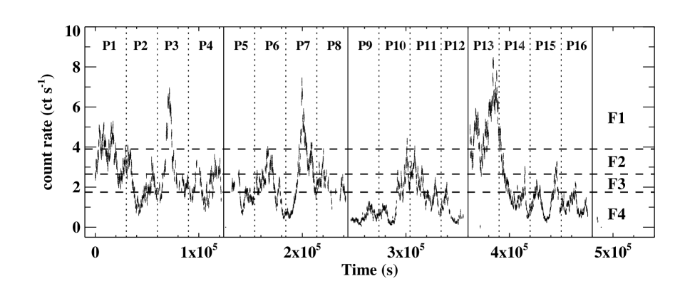
Figure 1: The figure shows the 0.3-10 keV EPIC PN light curves with a time bin of 200s. The dash lines in the figures show the count rate that we used to define different flux levels (see section 3.2 for details). The four orbits (divided by solid vertical lines) of entire observation were separated into 16 periods, each spanning an exposure of 30 ks. Note that time intervals between each orbit were discarded.

Reverberation of the soft excess was first detected in the extreme NLS1 1H 0707-495 (Fabian et al., 2009; Zoghbi et al., 2010). The soft X-rays lag behind the hard X-rays by 30 seconds, providing strong support for a disc reflection origin. In the standard reflection scenario, the hot corona above the accretion disc produces the primary powerlaw continuum, which irradiates the accretion disc and leads to the production of the reflection component. The soft lags can be understood as the time delay between the powerlaw (hard X-rays) and reflection (soft X-rays) components. Reverberation lags have since been observed in a number of AGN (Emmanoulopoulos et al., 2011; Zoghbi et al., 2012), and also present in stellar-mass black holes (Uttley et al., 2011). Although Legg et al. (2012) claimed that the reverberation lag is a consequence of scattering from distant (a few tens to hundreds of gravitational radii, $R_{\rm g}=GM/c^{2}$) material, more recent work suggests this process cannot be driving the complex lag phenomenology observed (Kara et al. 2013b; Walton et al. 2013b). The work of De Marco et al. (2013) showed that the characteristic time-scales of the reverberation lag are highly correlated with the black hole mass, indicating that soft lags originate from the innermost regions of the accretion flow. In addition, studies of X-ray microlensing have shown that the X-ray emitting region of quasars are compact (Morgan et al., 2012; Chartas et al., 2012; Chen et al., 2012), which is consistent with the sizes typically inferred in the reflection scenario. Furthermore, signatures of relativistic disc reflection have now been observed from the lensed quasar RX J1131-1231 (Reis et al. 2014), for which microlensing has independently constrained the size of the X-ray emitting region to be $R_{\rm X}\lesssim 10~{}R_{\rm g}$ (Dai et al. 2010). The relativistic reflection model offers a natural and self-consistent physical interpretation of both the timing and spectral properties of NLS1s.

IRAS13224-3809 (z=0.066, D $\sim 2.8\times 10^{8}$ pc) is a radio-quiet, extreme NLS1 which shows many similarities with 1H0707-495, including rapid variability. The $H\beta$ line properties (FWHM $\sim$ 650 km s^-1, flux$\sim 3.5\times 10^{-14}$ erg cm^-2 s^-1) obtained from optical observations (Boller et al., 1993) imply a black hole mass of $\sim 1.5\times 10^{7}M_{\odot}$ (Kaspi et al., 2000). The source was first observed with XMM-Newton in 2002, revealing both a large soft excess, and a sharp spectral curvature around 7-8 keV (Boller et al., 2003), similar to other extreme NLS1. In particular, strong, broad iron L emission was observed below $\sim$1 keV (Ponti et al., 2010), implying a strong overabundance of iron, again similar to 1H0707-495 (Fabian et al., 2009). In 2011, IRAS 13224-3809 was observed with XMM-Newton for 500 ks. The soft excess lags behind the harder continuum by $\sim$ 90 s (Fabian et al., 2013), again providing strong support for a relativistic reflection origin. Furthermore, a similar reverberation lag has now been detected from the broad Fe K emission, and the lag-frequency spectrum of IRAS 13224-3809 also displays remarkable similarity to that of 1H0707-495 (Kara et al., 2013a). The lag analysis also implies the mass of central black hole to be $\sim 10^{7}M_{\odot}$ (see also section 4.3). In this work, we use the latest 500 ks XMM-Newton observation and present detailed spectral analyses in order to further probe the behaviour of this remarkable source. Calculations in this paper were assumed a flat cold dark matter cosmology with $H_{\rm 0}$ = 71 km s^-1 Mpc^-1.

2 Data Reduction

IRAS 13224-3809 was observed with XMM-Newton during 2011 July 19-29 (Obs. IDs 0673580101, 0673580201, 0673580301, 0673580401) for $\sim$ 500 ks. Fig. 1 shows the 0.3-10.0 keV light curves of the European Photon Imaging Camara (EPIC) PN. The source is highly variable, varying by a factor of $\sim$ 8 during the observation. All data have been reduced using the Science Analysis Software (SAS) version 12.0.1 with latest calibration files. The EPIC was operated in full window imaging mode during the first observation, and in large window imaging mode in the following three observations. We extracted source spectra of EPIC MOS and PN using a circular region with a radius of 35 arcsec. Background spectra were extracted using a region with the same size from a source-free region. Some regions of the EPIC PN CCD are affected by the Cu-K lines from the electric circuits behind that cause contamination on the background at 8.0 and 8.9 keV, and these regions were avoided during background selection.

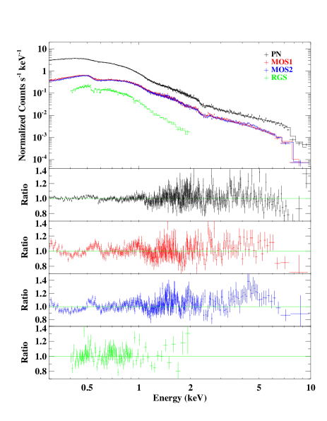
Figure 2: The figure shows the time-averaged EPIC and RGS spectra fitted with the best-fitting relativistic reflection model. These spectra have been re-binned for clarity. The PN, MOS1, MOS2, RGS data are presented using black, red, blue, and green points, respectively.

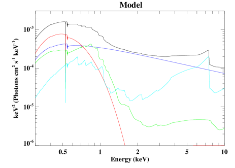
Figure 3: The figure shows the decomposed model used for fitting. The top black line stands for the combined model.

The spectrum of IRAS 13224-3809 is steep and background is important at high energies. Periods of high background were removed following the method outlined by Piconcelli et al. (2004), which determines the background threshold that maximises the signal-to-noise (S/N) in a chosen band; here we maximise the S/N for the full 0.3–10.0 keV EPIC bandpass. We obtained total of $\sim$ 350 ks, $\sim$ 401 ks, $\sim$ 407 ks of good exposure time for PN, MOS1, and MOS2, respectively. The redistribution matrix file (RMF) and the ancillary response file (ARF) were created using the RMFGEN and ARFGEN tools. We examined all the observations using the EPATPLOT task in SAS and found that they are not piled up. When necessary, spectra extracted from different orbits have been reduced separately, and then combined using ADDASCASPEC, part of the HEASOFT distribution. Only spectra of from same detector were combined. We rebinned the spectra to have a minimum of 30 counts in each energy bin using the GRPPHA tool. In this work, we use EPIC data over the full 0.3-10.0 keV bandpass, but note that there are few data points above $\sim$ 8 keV due to the high relative contribution of the background in this band, a consequence of the steep source spectrum (see Fabian et al. 2013).

We also reduced the Reflection Grating Spectrometer (RGS) data following the standard procedures. Both the first order spectra of RGS1 and RGS2 data were extracted. In order to analyse the data more efficiently, we used the RGSCOMBINE tool to combine RGS1 and RGS2 spectra into a single spectrum. We analyse the RGS spectrum over the 0.4-2.0 keV bandpass, which is broadly well-calibrated with the EPIC spectra.

3 Data Analysis and Comparison

3.1 Time-averaged Spectra

The initial analysis of time-averaged EPIC PN spectrum can be found in Fabian et al. (2013), and we begin by extending this time-averaged analysis to include the MOS and RGS data. Based on that used in Fabian et al. (2013), we construct a model to fit the EPIC and RGS spectra composed of a powerlaw continuum, two blurred reflection components, and a very soft blackbody component (BBODY), which contributes at the lowest energies probed. The double reflection components primarily account for the soft excess, and explain the $\sim$ 0.8 keV Fe L feature significantly better than the smooth curvature produced by Comptonization. Galactic absorption was modeled using the TBNEW neutral absorption code (Wilms et al., in preparation), with the solar abundances presented in Wilms et al. (2000). We used the EXTENDX grid, which is an extended version of the REFLIONX grid (Ross & Fabian, 2005) that allows for a wider range of iron abundance (0.1-20 times solar abundance), to model reflected emission. The RELCONV (Dauser et al., 2010) kernel acts on the reflected emission to account for relativistic effects. We assumed the inner edge of the accretion disc to extend down to the innermost stable circular orbit (ISCO), and the outer radius to be 400 $R_{g}$. Limb-darkening effects have been considered. The model is expressed as TBNEW*(POWERLAW + BBODY + RELCONV*(EXTENDX₁ + EXTENDX₂)), and fits the data well (see Fig. 3 and Table 1). The parameters obtained are generally consistent with those presented in Fabian et al. (2013), though the Galactic absorption column and iron abundance are slightly higher. These parameters are sensitive in the soft energy bands and cross-calibration differences between PN, MOS and RGS, the latter two now being included, may lead to mildly different best-fitting values.

Table 1: The table lists parameters of the best-fitting reflection model of EPIC and RGS spectra, in which $N_{\mbox{\scriptsize H}}$ is given in $10^{20}$ cm^-2, and $\xi$ in erg cm s^-1. The normalisation of the powerlaw component is expressed in photons keV^-1 cm^-2 s^-1, and that of the blackbody component in $10^{37}$ erg s^-1 kpc^-2. $F_{\rm BB}$ were calculated over the 0.01-10.0 keV band, while flux of other components were measured between 0.1 and 100 keV. The hard upper limit of $q_{1}$ is 10, and that of $A_{\rm Fe}$ is 20. The reflection fraction $\mathcal{R}$ is defined as (flux of reflector)/($F_{\rm RDC}$+$F_{\rm PLC}$).

Component	Parameter	powerlaw emissivity	broken powerlaw emissivity
TBNEW	Absorption column, $N_{\rm H}$	$6.3\pm 0.1$	$6.1^{+0.3}_{-0.1}$
BBODY	Temperature, $kT$ ($10^{-2}$ keV)	$9.4\pm 0.1$	$9.3^{+0.1}_{-0.2}$
	Norm	$(4.0\pm 0.1)\times 10^{-5}$	$3.6^{+0.3}_{-0.2}\times 10^{-5}$
	$F_{\rm BB}$ ($10^{-13}$ erg cm-2 s-1)	$33.4\pm 0.4$	$29.9^{+2.4}_{-1.2}$
POWERLAW	Photon index, $\Gamma$	$2.67^{+0.03}_{-0.01}$	$2.71\pm 0.02$
	Norm	$(3.7\pm 0.1)\times 10^{-4}$	$(3.8\pm 0.1)\times 10^{-4}$
	$F_{\rm PLC}$ ($10^{-13}$ erg cm-2 s-1)	$41.7\pm 0.3$	$43.3^{+1.2}_{-1.1}$
RELCONV	Inner emissivity index, $q_{1}$	$4.3^{+0.3}_{-0.1}$	$>9$
	Outer emissivity index, $q_{2}$	-	$3.4^{+0.3}_{-0.2}$
	Spin parameter, $a^{*}$	$>0.989$	$0.990^{+0.001}_{-0.003}$
	$R_{\rm break}$ ($R_{\rm g}$)	-	$2.1\pm 0.1$
	Inclination, $i$ (deg)	$64.9\pm 0.3$	$64.6^{+0.6}_{-0.7}$
EXTENDX	Iron abundance /solar, $A_{\rm Fe}$	$18.1\pm 0.7$	$>18.1$
	Ionization parameter, $\xi_{1}$	$499^{+3}_{-12}$	$498^{+4}_{-38}$
	${\rm Norm}_{1}$	$(1.7\pm 0.1)\times 10^{-8}$	$2.2^{+0.1}_{-0.3}\times 10^{-8}$
	$\mathcal{R}_{1}$	$\sim 0.32$	$\sim 0.33$
	Ionization parameter, $\xi_{2}$	$20.0^{+0.2}_{-0.6}$	$20.5^{+0.3}_{-1.1}$
	${\rm Norm}_{2}$	$4.6^{+0.8}_{-0.2}\times 10^{-6}$	$5.9^{+0.3}_{-0.9}\times 10^{-6}$
	$\mathcal{R}_{2}$	$\sim 0.14$	$\sim 0.15$
	$F_{\rm RDC}$ ($10^{-13}$ erg cm-2 s-1)	$36.5^{+0.5}_{-0.8}$	$41.0^{+1.3}_{-3.7}$
$\chi^{2}/d.o.f.$		3790/2890	3633/2892

The best-fitting parameters again show that IRAS 13224-3809 harbours a rapidly-spinning central black hole. The emissivity profile, i.e. the radial illumination of the accretion disc, is first assumed to have a powerlaw form, following $\epsilon(r)\propto r^{-q}$. We then tested a more sophisticated model with a broken powerlaw emissivity profile, which follows $\epsilon(r)\propto r^{-q_{1}}$ within some break radius $R_{\rm break}$, and $\epsilon(r)\propto r^{-q_{2}}$ outside that radius. We list results obtained from both models in Table 1 for comparison. The emissivity indices are similar to those presented in Fabian et al. (2013) as well. The steep inner emissivity index $q_{1}$ implies strong gravitational light-bending effects near the central black hole. There are some residuals around $\sim$ 0.5 keV and $\sim$ 1.4 keV in the EPIC spectra, which might be hints of absorption. However, these features are not present in the RGS spectrum, and no additional absorption components are required to model the data. The RGS spectrum does not show any distinct feature, and we conclude that the spectra of IRAS 13224-3809 are not modified by warm absorbers.

Analysis of the time-averaged spectra reveals the general spectral properties of IRAS 13224-3809. However, during the $\sim$ 500 ks observation, the source flux varies substantially. In order to investigate any spectral variability associated with this flux variability, we proceed to carry out a flux-resolved spectral analysis.

3.2 Flux-resolved Spectra

We divided the EPIC PN 0.3-10 keV light curves into four flux intervals, and extracted a spectrum from each. The dashed lines in Fig. 1 show the counts that have been chosen to develop the flux intervals. Each flux bin has a similar number of total counts ($\sim 1.9\times 10^{5}$). The same technique has been also used to investigate the spectral variability in MCG–6-30-15 (Vaughan & Fabian, 2004; Chiang & Fabian, 2011). We first examined the difference spectrum between the two highest flux states and the two lowest, i.e. the result of subtracting the low-flux (F3+F4) spectrum from the high-flux (F1+F2) spectrum. We modeled the difference spectrum with an absorbed powerlaw and found a clear soft excess below $\sim$ 1.5 keV (Fig. 4). The soft blackbody component of IRAS 13224-3809 may vary and cause the difference in the soft band between high and low-flux states. Alternatively, changes in the ionisation state of the blurred reflection component may also result in difference in the low-energy band. We found that the soft excess in the difference spectrum can be fitted either by including a blackbody component of $kT\sim 0.12$ keV or a reflection component, and further analysis is required to probe the real origin of this feature.

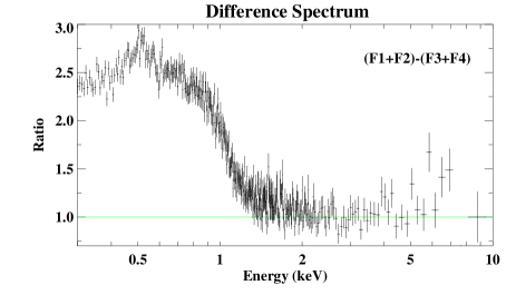
Figure 4: The figure shows the EPIC PN difference spectrum fitted with an absorbed powerlaw. A soft excess can be seen below $\sim$ 1 keV

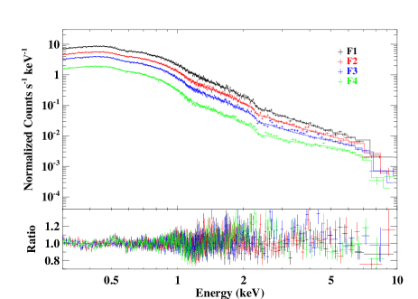
Figure 5: The figure shows the EPIC PN flux-resolved spectra fitted with the relativistic reflection model. Spectra of different flux states are shown using data points of different colours. These spectra have been re-binned for clarity.

Table 2: The table lists parameters of the best-fitting model of the flux-resolved spectra, where $N_{\mbox{\scriptsize H}}$ is also given in $10^{20}$ cm^-2, and $\xi$ in erg cm s^-1. Fluxes are again given in $10^{-13}$ erg cm^-2 s^-1, and $\xi$ in erg cm s^-1. If parameters are bound over the spectra, only values of F1 are listed. Since $\Gamma$ was restricted in a narrow range and easily to hit the hard limit when calculating uncertainties, we only list the best-fitting values.

Component	Parameter	Value
		F1	F2	F3	F4
TBNEW	$N_{\rm H}$	$6.9^{+0.4}_{-0.2}$	-	-	-
BBODY	$kT$ ($10^{-2}$ keV)	$9.6^{+0.2}_{-0.3}$	$9.3^{+0.3}_{-0.5}$	$8.8^{+0.2}_{-0.3}$	$8.3\pm 0.2$
	Norm	$7.4^{+0.6}_{-0.4}\times 10^{-5}$	$5.8^{+0.7}_{-0.5}\times 10^{-5}$	$(5.6\pm 0.3)\times 10^{-5}$	$(3.1\pm 0.2)\times 10^{-5}$
	$F_{\rm BB}$	$62.0$	$48.9$	$46.6$	$25.8$
POWERLAW	$\Gamma$	2.80	2.76	2.63	2.63
	Norm	$(1.2\pm 0.1)\times 10^{-3}$	$7.0^{+0.2}_{-0.3}\times 10^{-4}$	$(3.6\pm 0.1)\times 10^{-4}$	$(1.2\pm 0.1)\times 10^{-4}$
	$F_{\rm PLC}$	$151.5$	$84.3$	$38.7$	$13.1$
RELCONV	$q$	$3.2^{+0.6}_{-0.5}$	$3.8^{+0.4}_{-0.6}$	$4.1\pm 0.4$	$5.3^{+0.3}_{-0.4}$
EXTENDX	$A_{\rm Fe}$	$16.9^{+2.0}_{-1.1}$	-	-	-
	$\xi_{1}$	$990^{+70}_{-210}$	$500^{+90}_{-160}$	$260^{+300}_{-40}$	$220^{+80}_{-40}$
	${\rm Norm}_{1}$	$2.0^{+1.1}_{-0.3}\times 10^{-8}$	$3.2^{+2.9}_{-0.6}\times 10^{-8}$	$4.3^{+1.2}_{-2.3}\times 10^{-8}$	$3.5^{+2.2}_{-1.9}\times 10^{-8}$
	$\mathcal{R}_{1}$	$\sim 0.32$	$\sim 0.33$	$\sim 0.36$	$\sim 0.40$
	$\xi_{2}$	$20^{+1}_{-2}$	-	-	-
	${\rm Norm}_{2}$	$6.9^{+1.4}_{-1.7}\times 10^{-6}$	$6.4^{+2.7}_{-2.1}\times 10^{-6}$	$3.8^{+1.1}_{-0.4}\times 10^{-6}$	$3.6^{+0.4}_{-0.3}\times 10^{-6}$
	$\mathcal{R}_{2}$	$\sim 0.07$	$\sim 0.10$	$\sim 0.14$	$\sim 0.27$
	$F_{\rm RDC}$	$97.8$	$63.0$	$39.3$	$22.6$
$\chi^{2}/d.o.f.$		2214/2085

We simultaneously modeled the four flux-resolved spectra with the same model used for the time-averaged spectra in section 3.1. Since the exposure of each flux-resolved spectra is obviously substantially shorter than the time-averaged spectra, we use a simpler emissivity profile consisting of a single powerlaw to improve the efficiency of fitting and better constrain the parameters. Parameters which should remain constant on observational timescales, i.e. the black hole spin $a^{*}$ and the disc inclination angle $i$, have been fixed to the same values obtained in time-averaged analysis (Table 1). Since for this analysis we focus on the PN data only, the Galactic absorption column $N_{\rm H}$ and iron abundance $A_{\rm Fe}$ might be mildly different from those obtained from the combined fit to the PN, MOS and RGS time-averaged spectra. These parameters were allowed to vary overall, but were linked across each of the flux bins. We also linked the the ionisation parameter of the second reflection component ($\xi_{2}$, the lower one) as it showed no distinct evolution between different flux states.

The photon index of the powerlaw component $\Gamma$ has been found to vary by a few per cent with flux states in some NLS1s. In Fig. 5 it can be seen that the shape of each spectrum is fairly similar, which implies that photon index does not vary substantially between the different flux states. To confirm this, we fit the flux-resolved spectra between 1-2 keV, which is an energy band free of absorption and dominated by the powerlaw continuum, with a single powerlaw and find that $\Gamma$ varies in a small range ($\sim$ 3 per cent). We therefore restrict the photon index to be in the range of 2.63-2.8 (the best-fitting value $\Gamma=2.71$ from the time-averaged analysis $\pm$3%). Previous analyses of 1H0707-495 also found that the photon index varies within a small range (2.95-3.05) across different states.

The rest of the parameters in the model are allowed to vary between the different flux states, and the results are presented in Table 2. As shown in Fig. 5, the model works well on the flux-resolved spectra. It can clearly be seen that the photon index tends to be softer during high-flux states, and the normalisation of the powerlaw component decreases from high-flux states to low-flux states. The flux of reflection components seems to follow the same trend of the powerlaw component. The ionisation parameter of the first reflection component appears to be proportional to the flux of the powerlaw component. The changing ionisation parameter might be the cause of the soft excess present in the difference spectrum (Fig. 4). However, the blackbody component also appears to vary between different flux states and also contributes to the difference spectrum. The emissivity index appears to be steeper when fluxes are lower, implying more emission comes from the inner disc when the source is fainter.

3.3 Time-resolved Spectra

3.3.1 30 ks slices

In order to further probe the general trends of the source, we extracted a series of time-resolved spectra from each of the EPIC detectors, similar to recent analyses by Reis et al. (2012); Marinucci et al. (2014); Walton et al. (2014). Each interval spans a duration of 30 ks (see Fig. 1), giving 16 intervals in total. Note that the actual good time varies depending on the behaviour of the background. For each interval, we independently applied the model used previously in sections 3.1 and 3.2. Similar to our flux-resolved spectal analysis, parameters that should not vary on observational timescales were fixed to the best-fitting values from our time-averaged analysis (including now the iron abundance and the neutral absorption column, given the consistent set of detectors used for these analyses; see Table 1), and the photon index was again restricted to lie between $\Gamma=2.63-2.8$. These 16 periods cover a wide variety of flux states, providing additional data over a broad dynamic range with which to further examine the parameter trends obtained with our flux-resolved spectra. In Table 3 we list the best-fitting parameters obtained, along with the absorption-corrected 0.1-100.0 keV fluxes of the powerlaw continuum and the total reflected emission ($F_{\rm PLC}$ and $F_{\rm RDC}$ respectively), and the 0.01-10.0 keV absorption-corrected fluxes of the blackbody component ($F_{\rm BB}$). All fluxes were calculated using the CFLUX model in XSPEC.

Fig. 6 shows a series of plots examining the observed evolution for several of the key model parameters. It can been seen in Fig. 6a that the reflected flux correlates strongly with the powerlaw flux, although we note that the powerlaw flux varies over a larger range than the reflected flux does. Panels b-d show that the source becomes progressively reflection-dominated when it is fainter, and that the emissivity index also rises as the observed flux drops and the source becomes more reflection-dominated, consistent with the conclusions from the flux-resolved analysis.

In panels e and f we examine the behaviour of the blackbody component. First, we investigate the evolution of the temperature and luminosity of this component, and find that these parameters seem to broadly follow the $L\propto T^{4}$ relation expected for blackbody emission from a constant emitting area (black dash line in Fig. 6e). We first statistically confirm the correlation between these quantities by conducting a simple Spearman’s rank correlation test and found a Pearson correlation coefficient of $\sim$ 0.58, corresponding to a false-alarm probability of $\sim$ 0.0093. We then used the IDL routine MPFITEXY, an which relies in turn on the MPFIT package (Markwardt, 2009), to fit the data accounting for the uncertainties in both the luminosity and the temperature, and found a slope of $0.18\pm 0.04$ (red dot dash line in Fig. 6e), which is close to the expected value 0.25. The good agreement with the basic expectation for thermal emission supports a physical origin for the blackbody component. This may originate through heating of the inner accretion disc by the powerlaw continuum and/or the reflected emission; a more detailed discussion is given in section 4.2. We stress that although the blackbody component dominates in the observed bandpass of the soft excess, the broad iron L feature (see Fabian et al. 2013), is accounted for by the reflected emission. In Fig. 6f we plot fluxes of the powerlaw continuum and the reflected emission against the blackbody flux. It seems that $F_{\rm BB}$ is correlated with both $F_{\rm PLC}$ and $F_{\rm RDC}$. The Pearson correlation coefficients are $\sim$ 0.51 for $F_{\rm PLC}$ and $F_{\rm BB}$, and $\sim$ 0.69 for $F_{\rm RDC}$ and $F_{\rm BB}$.

Finally, while the results presented in Table 3 suggest the ionisation parameter of the first (higher ionisation) reflection component may correlate with the powerlaw flux, ultimately the ionisation of this component is not well constrained in our time-resolved analysis. Otherwise, these results help to confirm the trends found in the flux-resolved analysis, shedding further light on the extreme nature of this source.

Table 3: The table lists parameters of different periods (see Fig. 1) of data. The absorbed (absorption-corrected) fluxes of the blackbody $F_{\rm BB}$, powerlaw $F_{\rm PLC}$ and reflection components $F_{\rm RDC}$ are given in $10^{-13}$ erg cm^-2. $F_{\rm BB}$ were calculated over the 0.01-10.0 keV band, while $F_{\rm PLC}$ and $F_{\rm RDC}$ were measured between 0.1 and 100 keV. Temperatures of the blackbody component are given in 10^-2 keV, and $q$ states the emissivity index. Again we only list the best-fitting values of $\Gamma$ here.

Period	$\Gamma$	$kT_{\rm BB}$	$q$	$\xi_{\rm 1}$	$F_{\rm BB}$	$F_{\rm PLC}$	$F_{\rm RDC}$	$\mathcal{R}_{1}$	$\mathcal{R}_{2}$	$\chi^{2}_{\mu}$
		10-2 keV		erg cm s-1	10-13 erg cm-2 s-1					($\chi^{2}$/d.o.f.)
P1	$2.80$	$10.4\pm 0.3$	$4.5^{+0.5}_{-1.3}$	$970^{+120}_{-440}$	$33.2^{+4.2}_{-2.7}$	$105.2^{+2.2}_{-11.2}$	$58.3^{+7.6}_{-17.4}$	0.27	0.09	992/973
P2	$2.63$	$9.0\pm 0.3$	$4.6^{+0.6}_{-0.8}$	$320^{+210}_{-110}$	$35.3^{+2.4}_{-7.6}$	$33.9^{+0.8}_{-1.1}$	$33.0^{+4.6}_{-4.3}$	0.31	0.18	844/719
P3	$2.69$	$10.0^{+0.3}_{-0.4}$	$3.1^{+0.7}_{-0.5}$	$610^{+400}_{-140}$	$34.8^{+3.2}_{-4.8}$	$74.1^{+10.4}_{-7.8}$	$36.0^{+6.0}_{-6.1}$	0.25	0.08	720/719
P4	$2.63$	$9.5\pm 0.3$	$3.1^{+0.8}_{-0.5}$	$500^{+210}_{-220}$	$34.1^{+7.3}_{-4.2}$	$37.7^{+6.7}_{-1.3}$	$25.9^{+7.6}_{-3.1}$	0.29	0.12	627/592
P5	$2.80$	$7.8^{+0.9}_{-0.5}$	$5.2^{+0.5}_{-1.3}$	$970^{+120}_{-680}$	$22.1^{+7.2}_{-2.0}$	$45.6^{+1.6}_{-8.5}$	$35.6^{+11.4}_{-9.2}$	0.21	0.23	682/683
P6	$2.63$	$9.5^{+0.3}_{-0.4}$	$3.6\pm 1.0$	$520^{+220}_{-30}$	$24.5^{+1.3}_{-4.7}$	$37.8^{+6.9}_{-1.3}$	$22.9^{+8.9}_{-3.5}$	0.24	0.14	722/767
P7	$2.71$	$9.9\pm 0.2$	$3.2\pm 0.3$	$510^{+80}_{-90}$	$49.8^{+4.1}_{-5.6}$	$60.2^{+8.4}_{-6.3}$	$46.9^{+11.2}_{-9.0}$	0.32	0.12	921/859
P8	$2.63$	$9.2^{+0.4}_{-0.5}$	$3.6^{+1.7}_{-0.4}$	$220^{+100}_{-110}$	$41.0^{+3.6}_{-1.3}$	$20.8^{+3.5}_{-1.7}$	$29.6^{+13.2}_{-5.3}$	0.34	0.25	382/346
P9	$2.63$	$7.6^{+0.9}_{-1.0}$	$8.6^{+0.9}_{-0.4}$	$500^{+210}_{-310}$	$11.4\pm 1.4$	$5.6^{+0.4}_{-0.5}$	$16.8^{+5.5}_{-3.6}$	0.48	0.27	386/337
P10	$2.63$	$8.3\pm 0.4$	$7.0^{+0.5}_{-0.7}$	$500^{+130}_{-270}$	$32.1^{+1.3}_{-0.8}$	$17.2^{+0.6}_{-0.8}$	$36.7^{+5.5}_{-5.2}$	0.51	0.17	702/588
P11	$2.63$	$8.6^{+0.3}_{-0.2}$	$4.8^{+0.5}_{-0.4}$	$200^{+30}_{-60}$	$42.9^{+1.4}_{-2.3}$	$18.0\pm 0.9$	$37.4^{+5.2}_{-3.0}$	0.38	0.3	811/631
P12	$2.63$	$7.5^{+0.8}_{-0.7}$	$5.7^{+1.8}_{-1.0}$	$110^{+80}_{-50}$	$24.3\pm 5.1$	$6.2^{+1.0}_{-1.5}$	$24.2^{+8.3}_{-4.4}$	0.42	0.38	210/205
P13	$2.80$	$10.0\pm 0.2$	$3.6^{+0.5}_{-0.6}$	$1000^{+50}_{-340}$	$53.5^{+4.0}_{-2.5}$	$138.2^{+2.2}_{-6.1}$	$84.9^{+7.9}_{-4.9}$	0.28	0.1	1241/1087
P14	$2.63$	$9.2\pm 0.2$	$5.1^{+0.6}_{-0.7}$	$490^{+20}_{-280}$	$31.0^{+2.5}_{-2.1}$	$25.9^{+0.7}_{-0.9}$	$31.0^{+2.8}_{-4.2}$	0.31	0.23	815/704
P15	$2.63$	$8.9\pm 0.3$	$5.4^{+0.5}_{-0.3}$	$500^{+240}_{-230}$	$28.9^{+1.2}_{-0.6}$	$14.8^{+0.6}_{-0.7}$	$27.1^{+2.8}_{-3.0}$	0.32	0.33	649/577
P16	$2.63$	$8.6^{+0.4}_{-0.5}$	$6.0\pm 0.7$	$500^{+110}_{-290}$	$21.9\pm 1.9$	$12.6^{+0.6}_{-0.8}$	$25.6^{+2.2}_{-3.1}$	0.30	0.37	477/471

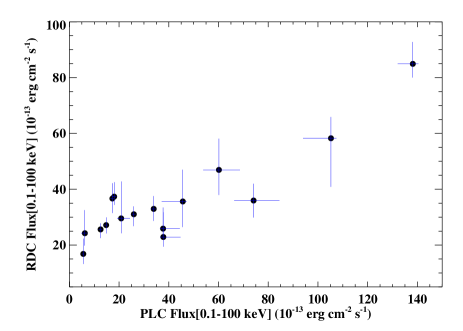
(a)

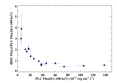
(b)

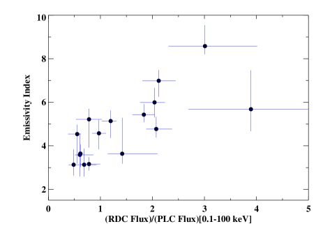
(c)

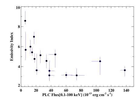
(d)

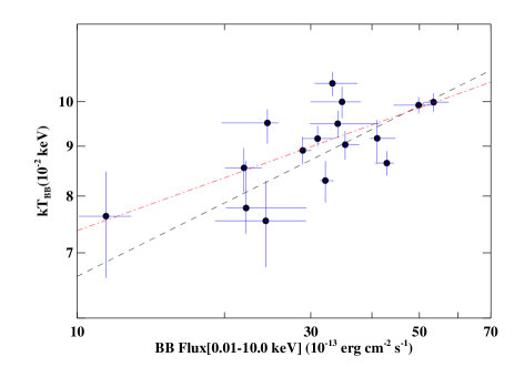
(e)

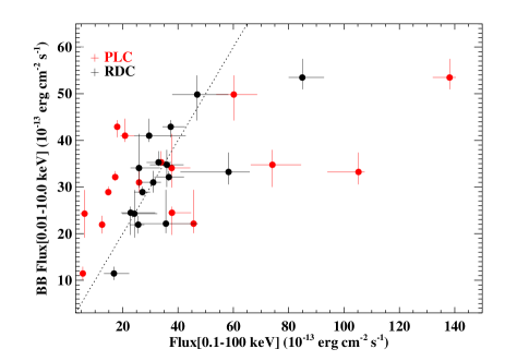
(f)

Figure 6: These figures show general trends of IRAS 13224-3809. PLC and RDC state for powerlaw component and reflection-dominated component, respectively. Fluxes were calculated over the 0.01-10.0 keV energy band for $F_{\rm BB}$, and over the 0.1-100 keV energy band for $F_{\rm PLC}$ and $F_{\rm RDC}$. The black dash line in figure (e) stands the $L\propto T^{4}$ relation and red dot dash line is drawn using the best-fitting slope ($0.18\pm 0.04$) of the data. The black dot line in figure (f) shows the expected relation when either $F_{\rm PLC}\propto F_{\rm BB}$ or $F_{\rm RDC}\propto F_{\rm BB}$ follows.

3.3.2 Normalized Light Curves

Our previous analyses examine how the source behaves between different flux states. We now extract the 0.3-1.0 keV (soft) and 1.2-5.0 keV (hard) PN light curves with 10-ks time bins to see how the hardness ratio (hard/soft) evolves during the observation. However, the count rates of the soft light curve are much larger than those of the hard light curve, so the hardness ratio remains small (slightly above 0; see upper panel in Fig. 7). In order to clearly visualise the evolution of hardness ratio, we normalised (subtracted the mean and divided by the standard deviation of the data) the soft (blue) and hard (red) light curves in Fig. 7. As some values of the soft light curve are also quite close to 0, the hardness ratio obtained from original light curves hits infinity even after normalisation. We instead calculated the colour (soft/hard) light curve and normalised it (lower panel in Fig. 7). The gaps between the four observations have been discarded.

Based on the behaviour of the normalised hardness ratio, it can be seen that the observation can be roughly separated into four different periods. We defined period 1 (N1) to be 0-175 ks, period 2 (N2) to be 175-330 ks, period 3 (N3) to be 330-405 ks, and period 4 (N4) to be 405-500 ks. In N1 and N3, the averages of soft/hard ratios (orange dash line in lower panel of Fig. 7) fall below 0, implying the source is generally harder during these periods, and softer during N2 and N4 (see also the orange dash lines in Fig. 7). These periods are roughly commensurate with those used in the time-dependent reverberation analysis presented by Kara et al. (2013a), allowing for direct comparison of the results obtained. For each of these periods, we extracted spectra from each of the EPIC detectors, and applied the model used previously. As before, parameters that are not expected to be time variable, e.g., $N_{\rm H}$, $a^{*}$, $i$, and $A_{\rm Fe}$, etc., are fixed at the best fit values from our time-averaged analysis, and we again use a simpler powerlaw form for the emissivity profile. The best-fit values for the remaining variable parameters are listed in Table 4 for each period.

As expected based on our previous analysis, the flux of the powerlaw increases and $\Gamma$ steepens during N1 and N3 (the higher flux periods). It is again clear that $F_{\rm RDC}$ shows less variability than $F_{\rm PLC}$, and is actually higher than $F_{\rm PLC}$ during N2 and N4. The inner emissivity profile appears to be steeper during N2 and N4, which is consistent with results of the flux-resolved and 30-ks time-resolved analyses. Again there is a hint that the ionisation parameter of the higher ionisation reflection component ($\xi_{1}$) correlates with the flux of the powerlaw component, but the values of N1, N2 and N4 are comparable and consistent within the 90 per cent confidence. In principle both the emissivity profile and disc ionisation parameter can give information of the position and size of the corona, and we will discuss this in detail in section 4.4.

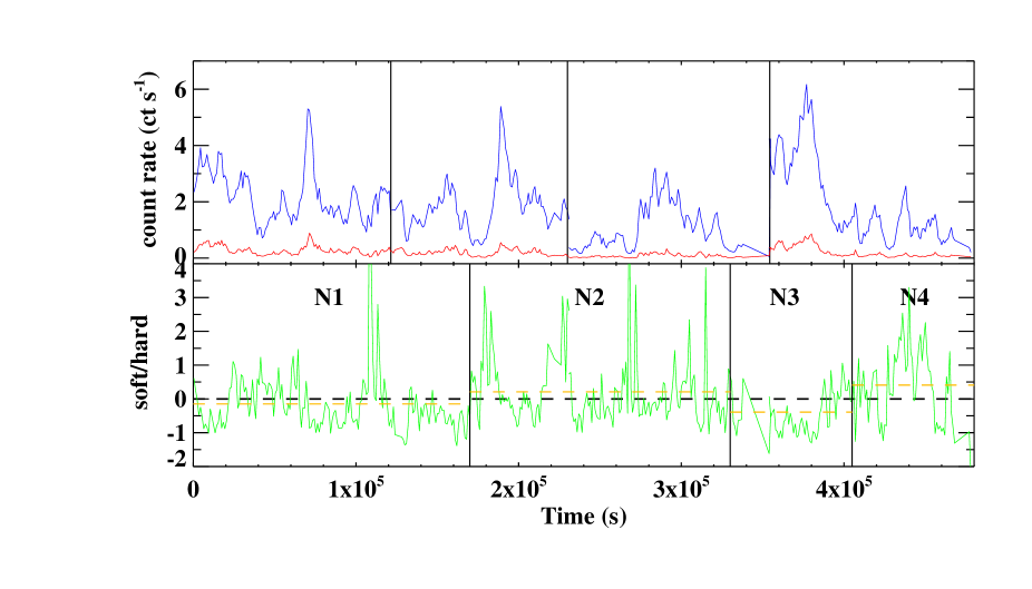
Figure 7: The figure shows normalized soft (0.3-1.0 keV; blue), hard (1.2-5.0 keV; red) and colour(soft/hard; green) light curves. The orange dash line represents the averaged value of the colour light curve in each segment. The time bin used in this plot is 1 ks.

Table 4: The table lists parameters of the best-fitting model of different periods which were selected using the normalised light curves (see Fig. 7). Fluxes are again given in $10^{-13}$ erg cm^-2 s^-1, and $\xi$ in erg cm s^-1. Parameters that are fixed at the same values with Table 1 are not listed here (see text).

Component	Parameter	Value
		N1	N2	N3	N4
BBODY	$kT$ (10-2 keV)	$9.6\pm 0.2$	$9.2^{+0.1}_{-0.2}$	$9.6\pm 0.2$	$8.8\pm 0.2$
	Norm	$3.9^{+0.3}_{-0.4}\times 10^{-5}$	$(4.0\pm 0.1)\times 10^{-5}$	$4.9^{+0.6}_{-0.2}\times 10^{-5}$	$(3.0\pm 0.1)\times 10^{-5}$
	$F_{\rm BB}$	$32.4^{+2.2}_{-2.7}$	$33.4^{+0.9}_{-0.4}$	$41.3^{+3.2}_{-2.1}$	$25.2^{+0.8}_{-0.4}$
POWERLAW	$\Gamma$	$2.69$	$2.63$	$2.80$	$2.63$
	Norm	$(5.3\pm 0.1)\times 10^{-4}$	$(2.2\pm 0.1)\times 10^{-4}$	$7.4^{+0.2}_{-0.1}\times 10^{-4}$	$(1.4\pm 0.1)\times 10^{-4}$
	$F_{\rm PLC}$	$59.3^{+2.0}_{-3.4}$	$23.4\pm 0.4$	$93.7^{+1.6}_{-7.3}$	$14.5^{+0.3}_{-0.5}$
RELCONV	$q$	$3.8^{+0.4}_{-0.5}$	$4.9\pm 0.2$	$4.1^{+0.4}_{-0.6}$	$5.8^{+0.3}_{-0.4}$
EXTENDX	$\xi_{1}$	$530\pm 70$	$500^{+10}_{-210}$	$830^{+190}_{-250}$	$500^{+100}_{-220}$
	${\rm Norm}_{1}$	$1.4^{+0.3}_{-0.2}\times 10^{-8}$	$1.5^{+1.1}_{-0.2}\times 10^{-8}$	$1.5^{+0.7}_{-0.3}\times 10^{-8}$	$1.0^{+0.7}_{-0.1}\times 10^{-8}$
	$\mathcal{R}_{1}$	$\sim 0.27$	$\sim 0.43$	$\sim 0.30$	$\sim 0.32$
	${\rm Norm}_{2}$	$4.6^{+1.5}_{-1.1}\times 10^{-6}$	$3.7^{+0.2}_{-0.3}\times 10^{-6}$	$9.9^{+1.0}_{-3.0}\times 10^{-6}$	$5.6^{+0.2}_{-0.4}\times 10^{-6}$
	$\mathcal{R}_{2}$	$\sim 0.11$	$\sim 0.13$	$\sim 0.13$	$\sim 0.33$
	$F_{\rm RDC}$	$36.5^{+5.8}_{-5.0}$	$29.8^{+0.6}_{-2.0}$	$69.9^{+6.2}_{-12.2}$	$27.2^{+2.8}_{-2.0}$
$\chi^{2}/d.o.f.$		1646/1475	1570/1225	1426/1194	1027/863

4 Discussion

We have presented various analyses of the spectral properties and in particular the strong spectral variability exhibited by IRAS13224-3809 during the long 500 ks XMM-Newton observation performed in 2011. The results obtained are well-explained by the relativistic reflection model initially presented in Ponti et al. (2010) and Fabian et al. (2013), and we confirm that IRAS13224-3809 hosts an almost maximally-rotating black hole. The reflected emission shows less variability than the powerlaw continuum, which is expected if gravitational light-bending effects are important. The model also includes a low temperature blackbody, which we find roughly follows the $L\propto T^{4}$ relation expected for stable thermal emission, suggesting this has a physical origin and is not just a phenomenological component included in the model to obtain good fits. We will further discuss the possible origin of this component in section 4.2. Our time-resolved analysis allows us to investigate how the spectral properties evolve between different flux levels, and we also discuss below how the source geometry may change by comparing results obtained from our spectral analyses and previous timing analyses (Kara et al. 2013a).

4.1 General Trends

In both the flux-resolved and time-resolved analyses we presented above, it is clear that the reflected emission shows less variability than the powerlaw continuum. $F_{\rm PLC}$ can vary by a factor of more than 10 during the entire observation (Table 3), while $F_{\rm RDC}$ only changes by a factor of $\sim$5. This agrees with the prediction of the gravitational light-bending model for a dynamic/geometrically evolving corona located in the region of strong gravity close to the black hole. Miniutti & Fabian (2004) showed that, for a simple lamppost disc–corona geometry, if the variability observed from the intrinsic X-ray source is related to changes in its proximity to the black hole, the reflection component should remain relatively constant due to gravitational light bending effects, as with a greater proximity, more of the X-ray emission is bent towards the black hole and lost over the event horizon rather than ‘seen’ by the disc. The same phenomena has been observed in a number of other Type 1 AGN (e.g. Vaughan & Fabian 2004; Fabian et al. 2012), and also in the Galactic black hole binary XTE J1650-500 (e.g. Rossi et al. 2005; Reis et al. 2013). In this scenario, since the reflection component should show less variability than the powerlaw continuum, when the observed flux from the source decreases it should progressively become more reflection-dominated, consistent with our spectral decomposition.

Assuming a compact, isotropic source above the accretion disc, the emissivity of the reflected emission from the disc would naturally decrease with increasing radius. In the simplest case without considering any relativistic effects, an emissivity index of $\sim$3 is expected (Reynolds & Begelman, 1997). However, in general relativity, if the X-ray source is close to the black hole, photons from the X-ray source are bent towards the central black hole and inner disc. As a result, the closer the source is to the black hole, the more the inner disc is preferentially illuminated, resulting in steeper emissivity profiles. More details of how relativistic effects modify the emissivity profile around AGN can be found in Wilkins & Fabian (2012), but the basic expectation is that increasingly reflection-dominated states should be accompanied by increasingly steep emissivity indices. Again, our spectral decomposition returns exactly this result; as shown in Fig. 6 (panels c and d), the emissivity index becomes steeper as $F_{\rm RDC}/F_{\rm PLC}$ increases and as the observed flux of the powerlaw continuum decreases.

4.2 The Blackbody Component

A blackbody component is sometimes used to fit the spectrum of AGN phenomenologically to explain the soft excess, but this component is not necessarily generated by the accretion disc. It is common to see the blackbody emission from the accretion disc in the X-ray spectrum of stellar-mass black holes (e.g. Remillard & McClintock 2006; Done et al. 2007). However in AGN, due to a much larger black hole mass, the accretion disc is cool and the blackbody component usually peaks in the EUV band with a temperature of a few eV. For AGN with a very massive central black hole, the inclusion of a blackbody component when fitting an X-ray spectrum is a way to model a soft excess of unknown origin. However, for AGN with relatively small central black holes and high accretion rates (e.g. NLS1s), the disc blackbody component can extend into the soft X-ray band. As an extreme NLS1, it is possible that the soft X-ray blackbody component of IRAS13224-3809 originates from the accretion disc.

Another possibility is that the inner part of the accretion disc is irradiated by a combination of direct coronal emission and returning radiation, heating it sufficiently to cause a blackbody component to appear in the soft X-ray band. Strong gravitational light-bending effects take place when the spin $a^{*}$ $>$ 0.9 causing some of the radiation from the accretion disc (thermal photons, reflection, etc.) to return to the disc, resulting in modifications in the spectrum (Cunningham 1976). Since IRAS 13224-3809 has a high spin, effects caused by returning radiation may be important. If the accretion disc is heated by either coronal photons or reflected photons then the blackbody component should be driven by the powerlaw or reflection component. In Fig. 6f, it appears that $F_{\rm BB}$ is correlated to both $F_{\rm PLC}$ and $F_{\rm RDC}$, though stronger with the latter.

Returning radiation causes multiple X-ray reflection (Ross et al. 2002) which creates additional spectral components in the final X-ray spectrum. The soft X-ray spectrum is steeper and featureless and the K-shell emission/absorption features of iron strengthen. Ross et al. (2002) demonstrated that multiple reflection could enhance the flux in the soft X-ray band, producing results similar to those caused by a blackbody component.

4.3 The Black Hole Mass

With knowledge of the distance and inclination of IRAS13224-3809, we can attempt to deduce the mass of the central black hole from the blackbody emission, given this appears to follow $L\propto T^{4}$ relation, implying a constant emitting area. Since the emission comes from the region affected by strong gravity, relativistic effects should be considered. The BBODY model gives the colour temperature of the blackbody component. A spectral hardening factor $f_{\rm col}$ should be included to obtain the effective temperature ($T_{\rm eff}\times f_{\rm col}=T_{\rm col}$). A typical $f_{\rm col}$ of 1.7 has been commonly used (Shimura & Takahara, 1995) and works well on stellar-mass black holes in the disc dominated state. In the case of NLS1s, however, the colour temperature correction could be as large as $\sim$2.4 (Ross et al., 1992; Done et al., 2012). The energy flux released from the accretion disc is related to the central black hole mass $M_{\rm BH}$. By measuring the disc flux, with the appropriate relativistic corrections, $M_{\rm BH}$ can be obtained. Li et al. (2005) introduced the KERRBB model, which calculates the emission from a multi-temperature, steady state, general relativistic accretion disc around a Kerr black hole. We replaced the BBODY component with KERRBB model and re-fit the time-averaged spectrum to estimate the black hole mass. The inclination, spin parameter and distance have been fixed to the best-fitting values of the time-averaged analysis (Table 1, broken powerlaw emissivity) for consistency. Assuming $f_{\rm col}$ = 2.4, we obtained a mass of $M_{\rm BH}=3.5^{+5.5}_{-0.6}\times 10^{6}M_{\odot}$ and an effective mass accretion rate of $2.74^{+0.14}_{-0.38}\times 10^{23}$g s^-1, which imply the $L/L_{\rm Edd}$ to be $\sim$0.23. The KERRBB gives a flux of $\sim 2.6\times 10^{-17}$ erg cm^-2 s^-1 Å^-1 at 2310Å, which significantly under-predicts the OM UVM2 flux $3.07\times 10^{-15}$ erg cm^-2 s^-1 Å^-1. The best-fitting black hole mass is smaller than the expected value $\sim 10^{7}M_{\odot}$ obtained from the reverberation analysis (Kara et al. 2013a), though the upper limit is close. The $\sim$90 s soft lag detected in IRAS13224-3809 implies that the source should be roughly three times more massive than 1H0707-495, which harbours a black hole of $M_{\rm BH}\sim 7\times 10^{6}M_{\odot}$.

The discrepancy in the black hole mass between spectral and timing analyses may indicate the origin of the blackbody component. Note that the KERRBB model uses the Novikov-Thorne profile for calculation. If the blackbody component is not induced by emission coming directly from the accretion disc, the black hole mass obtained from KERRBB is not valid and other method should be used for mass estimation. It is possible that the blackbody component is produced by irradiation or returning radiation mentioned in section 4.2. Although these alternatives cannot be examined by current models, the much smaller black hole mass obtained from spectral analysis and the underestimation of optical flux, may be hints of irradiation or returning radiation.

4.4 The Size of the Corona

Kara et al. (2013a) discovered that the reverberation lag from the soft excess has a larger amplitude (by a factor of $\sim$3) during high-flux states, and occurs on slightly longer timescales. This can be explained if the corona becomes more extended during high-flux states. Furthermore, in the case of the Galactic binary XTE J1650-500, Reis et al. (2013) also argue the characteristic size of the corona that is changing, through study of the simultaneous evolution of the reflected emission and the quasi-periodic oscillations exhibited by the coronal emission. Since the reverberation lag is relatively insensitive for a corona expanding radially with a constant vertical extent (Wilkins & Fabian, 2013), the result implied that the corona is more vertically-extended when brighter. The high-flux states in Kara et al. (2013a) are comparable with the periods N1 and N3 defined in section 3.3.2, and the low-flux states similar with N2 and N4, although we note that N1 has a much longer exposure than the low flux period examined by Kara et al. (2013a).

In principle, it may also be possible to determine the scale height of the corona from the ionisation of the accretion disc, which is defined as $\xi=L_{\rm ion}/nR^{2}$, where $L_{\rm ion}$ is the ionising luminosity, $n$ is the hydrogen number density of the disc, and $R$ is the distance between the source and the disc. Under the assumption that $n$ does not vary substantially within a short period of time, changes in $\xi$ imply either changes in the height of the corona, or changes in the intrinsic ionising luminosity from the corona. If the corona is more vertically-extended during high-flux states, and $L_{\rm ion}$ remains constant (i.e. the observed variability is driven by changes in source geometry rather than intrinsic luminosity, as suggested above), one might naively expect that $\xi$ should be lower for N1 and N3, and higher for N2 and N4, given the change in the characteristic distance between the inner disc and the corona. Instead, the ionisation parameter of the first (higher ionisation) reflection component seems to be positively correlated with the observed powerlaw flux (although $\xi_{1}$ for N1 is not significantly higher than that of N2 and N4, a positive correlation is also implied by the analysis presented in section 3.2, which covers a broader range of flux states).

However, this expectation does not fully account for the effects of gravitational lightbending, as it does not take into account the accitional continuum flux lost to the black hole. The ionisation parameter can be re-written as $\xi=F_{\rm incident}/n$, where $F_{\rm incident}$ is the incident flux as seen by the inner disc. If the albedo of the disc remains constant, changes in $F_{\rm incident}$ are actually best probed by changes in the reflected flux $F_{\rm RDC}$. Thus, based on the predictions of the gravitational lightbending model, one should in fact expect that even if the intrinsic ionising luminosity from the corona is constant, the ionisation of the disc should be higher when the flux is higher, as in the regime of strong gravitational lightbending the reflected flux and the observed powerlaw flux should be positively correlated (zone 1 in Figure 2 of Miniutti & Fabian 2004). Given the positive correlation between $F_{\rm PLC}$ and $F_{\rm RDC}$ observed, and the apparent positive correlation between $\xi_{1}$ and $F_{\rm PLC}$, these results would seem to be consistent with the corona being more extended when the flux is brighter.

Additionally, the evolution of the emissivity index can also help to constrain the evolution of the corona. As discussed previously, the emissivity index is steeper when the source is fainter and more reflection-dominated (see Figure 6). This also indicates the corona is likely becoming more compact in the lower flux periods, resulting in stronger lightbending. Focusing again on the periods highlighted in section 3.3.2 for direct comparison with Kara et al. (2013a), we again see evidence for the same trend (Table 4), albeit over a smaller dynamic range than probed with the analyses presented in sections 3.2 and 3.3.1. We also tried replacing the RELCONV convolution kernel with the RELCONV_LP version (Dauser et al. 2013), which assumes a lamp-post geometry for the corona, i.e. a point source located at some height $H$ above the spin axis of the black hole. Rather than fit the emissivity profile with a simple parameterisation, this model allows the height of the point source to be fit directly, and self-consistently computes the emissivity profile for that geometry.

As expected, applying this to the hardness-selected spectra (N1-4; section 3.3.2) we find that the height obtained for the corona is larger in the higher flux states (N2, N4) than in the lower flux states (N1, N3), evolving from $\sim$2 $R_{\rm g}$ to $\sim$3 $R_{\rm g}$. Making the same replacement for the flux-resolved spectra (F1-4; section 3.2), we see the same trend, with the corona height systematically evolving from $\sim$2 $R_{\rm g}$ in the lowest flux state to $\sim$4 $R_{\rm g}$ in the highest. Although the trend is exactly as expected for a corona that is larger in higher flux states, the range inferred for $H$ from RELCONV_LP is slightly smaller than inferred from the reverberation analysis (Kara et al. 2013a). However, the point source geometry assumed by RELCONV_LP is an obvious over-simplification, particularly for the scenario suggested in Kara et al. (2013a), in which the corona has some extent and its characteristic size evolves with flux. Therefore, even though there is some tension between the exact quantitative evolution of the corona between the spectral results obtained with RELCONV_LP and the reverberation analysis, the fact that both imply the same general evolution is very encouraging for this interpretation.

5 Conclusions

We have presented a detailed analysis of the spectral properties, and in particular the spectral variability exhibited by the extremely variable NLS1 IRAS13224-3809 during the long XMM-Newton observation obtained in 2011. For the latter, we investigate how the spectrum evolves by examining different states selected on both flux and a spectral hardness, as well as undertaking a systematic time-resolved spectral analysis. These spectra are interpreted in the context of the well established relativistic disc reflection model, based on recent works by Ponti et al. (2010) and Fabian et al. (2013). We find that the reflected emission from the disc is much less variable than the powerlaw continuum, and as the source flux drops, the spectrum becomes progressively more reflection-dominated. Furthermore, as the source becomes more reflection-dominated, the emissivity index simultaneously steepens. These trends are exactly as expected if the variability is dominated by a compact, centrally located X-ray corona which contracts as the source flux drops, resulting in increased gravitational lightbending which in turn produces more reflection-dominated states, and increases the preferential illumination of the innermost accretion disc. This is also broadly consistent with the observed evolution of the X-ray reverberation properties (Kara et al. 2013a), which strongly supports this interpretation.

Finally, the best-fit model also includes a contribution from a very soft blackbody. We find this appears to follow the expected $L\propto T^{4}$ relation for thermal emission from a stable emitting region, supporting a physical (rather than phenomenological) origin for this emission component. Given the high spin obtained for IRAS13224-3809 and the clear influence of gravitational lightbending, this may be related to heating of the inner disc by both radiation from the corona, and from ‘returning’ radiation originating emitted/reflected by the disc which is bent back towards the disc surface.

References

- Boller et al. (1997) Boller T., Brandt W. N., Fabian A. C., Fink H. H., 1997, MNRAS, 289, 393
- Boller et al. (2003) Boller T., Tanaka Y., Fabian A., Brandt W. N., Gallo L., Anabuki N., Haba Y., Vaughan S., 2003, MNRAS, 343, L89
- Boller et al. (1993) Boller T., Truemper J., Molendi S., Fink H., Schaeidt S., Caulet A., Dennefeld M., 1993, A&A, 279, 53
- Chartas et al. (2012) Chartas G., Kochanek C. S., Dai X., Moore D., Mosquera A. M., Blackburne J. A., 2012, ApJ, 757, 137
- Chen et al. (2012) Chen B., Dai X., Kochanek C. S., Chartas G., Blackburne J. A., Morgan C. W., 2012, ApJ, 755, 24
- Chiang & Fabian (2011) Chiang C.-Y., Fabian A. C., 2011, MNRAS, 414, 2345
- Crummy et al. (2006) Crummy J., Fabian A. C., Gallo L., Ross R. R., 2006, MNRAS, 365, 1067
- Cunningham (1976) Cunningham C., 1976, ApJ, 208, 534
- Dai et al. (2010) Dai X., Kochanek C. S., Chartas G., Kozłowski S., Morgan C. W., Garmire G., Agol E., 2010, ApJ, 709, 278
- Dauser et al. (2013) Dauser T., Garcia J., Wilms J., Böck M., Brenneman L. W., Falanga M., Fukumura K., Reynolds C. S., 2013, MNRAS, 430, 1694
- Dauser et al. (2010) Dauser T., Wilms J., Reynolds C. S., Brenneman L. W., 2010, MNRAS, 409, 1534
- De Marco et al. (2013) De Marco B., Ponti G., Cappi M., Dadina M., Uttley P., Cackett E. M., Fabian A. C., Miniutti G., 2013, MNRAS, 431, 2441
- Done et al. (2012) Done C., Davis S. W., Jin C., Blaes O., Ward M., 2012, MNRAS, 420, 1848
- Done et al. (2007) Done C., Gierliński M., Kubota A., 2007, A&A Rev., 15, 1
- Emmanoulopoulos et al. (2011) Emmanoulopoulos D., McHardy I. M., Papadakis I. E., 2011, MNRAS, 416, L94
- Fabian et al. (2013) Fabian A. C., Kara E., Walton D. J., Wilkins D. R., Ross R. R., Lozanov K., Uttley P., Gallo L. C., Zoghbi A., Miniutti G., Boller T., Brandt W. N., Cackett E. M., Chiang C.-Y., Dwelly T., Malzac J., Miller J. M., Nardini E., Ponti G., Reis R. C., Reynolds C. S., Steiner J. F., Tanaka Y., Young A. J., 2013, MNRAS, 429, 2917
- Fabian et al. (2004) Fabian A. C., Miniutti G., Gallo L., Boller T., Tanaka Y., Vaughan S., Ross R. R., 2004, MNRAS, 353, 1071
- Fabian et al. (2009) Fabian A. C., Zoghbi A., Ross R. R., Uttley P., Gallo L. C., Brandt W. N., Blustin A. J., Boller T., Caballero-Garcia M. D., Larsson J., Miller J. M., Miniutti G., Ponti G., Reis R. C., Reynolds C. S., Tanaka Y., Young A. J., 2009, Nature, 459, 540
- Fabian et al. (2012) Fabian A. C., Zoghbi A., Wilkins D., Dwelly T., Uttley P., Schartel N., Miniutti G., Gallo L., Grupe D., Komossa S., Santos-Lleó M., 2012, MNRAS, 419, 116
- Gallo (2006) Gallo L. C., 2006, MNRAS, 368, 479
- Gallo et al. (2004) Gallo L. C., Tanaka Y., Boller T., Fabian A. C., Vaughan S., Brandt W. N., 2004, MNRAS, 353, 1064
- Gierliński & Done (2004) Gierliński M., Done C., 2004, MNRAS, 349, L7
- Gierliński & Done (2006) —, 2006, MNRAS, 371, L16
- Jin et al. (2012) Jin C., Ward M., Done C., Gelbord J., 2012, MNRAS, 420, 1825
- Kara et al. (2013a) Kara E., Fabian A. C., Cackett E. M., Miniutti G., Uttley P., 2013a, MNRAS, 430, 1408
- Kara et al. (2013b) Kara E., Fabian A. C., Cackett E. M., Uttley P., Wilkins D. R., Zoghbi A., 2013b, MNRAS, 434, 1129
- Kaspi et al. (2000) Kaspi S., Smith P. S., Netzer H., Maoz D., Jannuzi B. T., Giveon U., 2000, ApJ, 533, 631
- Legg et al. (2012) Legg E., Miller L., Turner T. J., Giustini M., Reeves J. N., Kraemer S. B., 2012, ApJ, 760, 73
- Li et al. (2005) Li L.-X., Zimmerman E. R., Narayan R., McClintock J. E., 2005, ApJS, 157, 335
- Marinucci et al. (2014) Marinucci A., Matt G., Miniutti G., Guainazzi M., Parker M. L., Brenneman L., Fabian A. C., Kara E., Arevalo P., Ballantyne D. R., Boggs S. E., Cappi M., Christensen F. E., Craig W. W., Elvis M., Hailey C. J., Harrison F. A., Reynolds C. S., Risaliti G., Stern D. K., Walton D. J., Zhang W., 2014, ApJ, 787, 83
- Markwardt (2009) Markwardt C. B., 2009, in Astronomical Society of the Pacific Conference Series, Vol. 411, Astronomical Data Analysis Software and Systems XVIII, Bohlender D. A., Durand D., Dowler P., eds., p. 251
- Miniutti & Fabian (2004) Miniutti G., Fabian A. C., 2004, MNRAS, 349, 1435
- Morgan et al. (2012) Morgan C. W., Hainline L. J., Chen B., Tewes M., Kochanek C. S., Dai X., Kozlowski S., Blackburne J. A., Mosquera A. M., Chartas G., Courbin F., Meylan G., 2012, ApJ, 756, 52
- Nardini et al. (2011) Nardini E., Fabian A. C., Reis R. C., Walton D. J., 2011, MNRAS, 410, 1251
- Piconcelli et al. (2004) Piconcelli E., Jimenez-Bailón E., Guainazzi M., Schartel N., Rodríguez-Pascual P. M., Santos-Lleó M., 2004, MNRAS, 351, 161
- Ponti et al. (2010) Ponti G., Gallo L. C., Fabian A. C., Miniutti G., Zoghbi A., Uttley P., Ross R. R., Vasudevan R. V., Tanaka Y., Brandt W. N., 2010, MNRAS, 406, 2591
- Pounds et al. (1995) Pounds K. A., Done C., Osborne J. P., 1995, MNRAS, 277, L5
- Reis et al. (2012) Reis R. C., Fabian A. C., Reynolds C. S., Brenneman L. W., Walton D. J., Trippe M., Miller J. M., Mushotzky R. F., Nowak M. A., 2012, ApJ, 745, 93
- Reis et al. (2013) Reis R. C., Miller J. M., Reynolds M. T., Fabian A. C., Walton D. J., Cackett E., Steiner J. F., 2013, ApJ, 763, 48
- Reis et al. (2014) Reis R. C., Reynolds M. T., Miller J. M., Walton D. J., 2014, Nature, 507, 207
- Remillard & McClintock (2006) Remillard R. A., McClintock J. E., 2006, ARA&A, 44, 49
- Reynolds & Begelman (1997) Reynolds C. S., Begelman M. C., 1997, ApJ, 488, 109
- Risaliti et al. (2013) Risaliti G., Harrison F. A., Madsen K. K., Walton D. J., Boggs S. E., Christensen F. E., Craig W. W., Grefenstette B. W., Hailey C. J., Nardini E., Stern D., Zhang W. W., 2013, Nature, 494, 449
- Ross & Fabian (2005) Ross R. R., Fabian A. C., 2005, MNRAS, 358, 211
- Ross et al. (2002) Ross R. R., Fabian A. C., Ballantyne D. R., 2002, MNRAS, 336, 315
- Ross et al. (1992) Ross R. R., Fabian A. C., Mineshige S., 1992, MNRAS, 258, 189
- Rossi et al. (2005) Rossi S., Homan J., Miller J. M., Belloni T., 2005, MNRAS, 360, 763
- Schurch & Done (2007) Schurch N. J., Done C., 2007, MNRAS, 381, 1413
- Shimura & Takahara (1995) Shimura T., Takahara F., 1995, ApJ, 445, 780
- Uttley et al. (2011) Uttley P., Wilkinson T., Cassatella P., Wilms J., Pottschmidt K., Hanke M., Böck M., 2011, MNRAS, 414, L60
- Vaughan & Fabian (2004) Vaughan S., Fabian A. C., 2004, MNRAS, 348, 1415
- Walton et al. (2013a) Walton D. J., Nardini E., Fabian A. C., Gallo L. C., Reis R. C., 2013a, MNRAS, 428, 2901
- Walton et al. (2014) Walton D. J., Risaliti G., Harrison F. A., Fabian A. C., Miller J. M., Arevalo P., Ballantyne D. R., Boggs S. E., Brenneman L. W., Christensen F. E., Craig W. W., Elvis M., Fuerst F., Gandhi P., Grefenstette B. W., Hailey C. J., Kara E., Luo B., Madsen K. K., Marinucci A., Matt G., Parker M. L., Reynolds C. S., Rivers E., Ross R. R., Stern D., Zhang W. W., 2014, ArXiv e-prints
- Walton et al. (2013b) Walton D. J., Zoghbi A., Cackett E. M., Uttley P., Harrison F. A., Fabian A. C., Kara E., Miller J. M., Reis R. C., Reynolds C. S., 2013b, ApJ, 777, L23
- Wilkins & Fabian (2012) Wilkins D. R., Fabian A. C., 2012, MNRAS, 424, 1284
- Wilkins & Fabian (2013) —, 2013, MNRAS, 430, 247
- Wilms et al. (2000) Wilms J., Allen A., McCray R., 2000, ApJ, 542, 914
- Zoghbi et al. (2012) Zoghbi A., Fabian A. C., Reynolds C. S., Cackett E. M., 2012, MNRAS, 422, 129
- Zoghbi et al. (2010) Zoghbi A., Fabian A. C., Uttley P., Miniutti G., Gallo L. C., Reynolds C. S., Miller J. M., Ponti G., 2010, MNRAS, 401, 2419