Prescription for choosing an interpolating function

Abstract:

Interpolating functional method is a powerful tool for studying the behavior of a quantity in the intermediate region of the parameter space of interest by using its perturbative expansions at both ends. Recently several interpolating functional methods have been proposed, in addition to the well-known Padé approximant, namely the “Fractional Power of Polynomial” (FPP) and the “Fractional Power of Rational functions” (FPR) methods. Since combinations of these methods also give interpolating functions, we may end up with multitudes of the possible approaches. So a criterion for choosing an appropriate interpolating function is very much needed. In this paper, we propose reference quantities which can be used for choosing a good interpolating function. In order to validate the prescription based on these quantities, we study the degree of correlation between “the reference quantities” and the “actual degree of deviation between the interpolating function and the true function” in examples where the true functions are known.

1 Introduction

In theoretical physics, perturbative expansions are very often used to analyze the behavior of physical quantities with respect to the parameter of interest. But such perturbative expansions are insufficient for understanding the behavior of the physical quantities in the entire region of the parameter space. Although numerical simulations are often applied for computing such quantities in a wide range of parameter region, they are not always very easy to work out. In some situations, the expansions of the quantities in both ends (small end and large end, where the small end corresponds to small value of parameter and the large end corresponds to large value of parameter) are known, then interpolating functional methods can be used to provide an interpolating function which can approximate behavior of the quantities over the entire region of the parameter space. The Padé approximant is a well-known example for such an interpolating method, which can be used to find an appropriate interpolating function. Recently other interpolating methods also have been proposed. Namely, the “Fractional Power of Polynomial” (FPP) method [5] and the “Fractional Power of Rational function” (FPR) [1]. Since combinations of these methods also give interpolating functions, we may end up with multitudes of the possible approaches. This multitude of interpolating functions causes so-called the “landscape problem” such that we easily get lost which among multitudes of the interpolating functions. So a criterion for choosing an appropriate interpolating function is inevitable. Proposing an efficient criterion is the aim of this paper.

In this paper, we will propose several quantities as the reference quantities for selecting a good interpolating function. Because the interpolating functions will be applied when the information of the actual function of physical quantities are absent, these reference quantities should be constructed only by using the perturbative expansions and the interpolating functions. To check whether these quantities work as good references, we need to check the correlation between the set of these quantities and the “actual deviation between the true function $F(g)$ and its interpolating function $G(g)$”, where $g$ is a parameter of interest. To see the correlation, we will calculate the correlation coefficients between them. Though also [1] has suggested a criterion, we will argue that their criterion was insufficient. Because as explained in Appendix A, they did not analyze the above mentioned correlations properly.

This paper is organized as follows: In section 2, we introduce the interpolating functions, the landscape problem and need of criteria for selecting a good interpolating function. In subsection 2.3, we introduce the correlation coefficients. In section 3, we will suggest the reference quantities for selecting a good interpolating function. In section 4, we examine the reference quantities by computing the correlation coefficients in examples where the actual functions are known. Section 5 is conclusion and summary.

2 Preliminary

2.1 Interpolating functions

Let us consider a function $F(g)$ defined in $g\in[0,\infty)$, which has $N_{s}$ order small-$g$ expansion $F_{s}^{(N_{s})}(g)$ around $g=0$ and $N_{l}$ order large-$g$ expansion $F_{l}^{(N_{l})}(g)$ around $g=\infty$. The forms of the expansions are

$$F_{s}^{(N_{s})}(g)=g^{a}\sum_{k=0}^{N_{s}}s_{k}g^{k},\quad F_{l}^{(N_{l})}(g)=g^{b}\sum_{k=0}^{N_{l}}l_{k}g^{-k}.$$ (2.1)

We expect that

$$F(g)-F_{s}^{(N_{s})}(g) ={\cal O}(g^{a+N_{s}+1}),\mbox{$$}$$

$$F(g)-F_{l}^{(N_{l})}(g) =\mathcal{O}(g^{b-N_{l}-1}),$$ (2.2)

around $g=0$ and $g=\infty$ respectively. Based on these expansions, we construct smooth interpolating functions whose small-$g$ and large-$g$ expansions coincide to the expansions (2.1) up to some orders.

2.1.1 Padé approximant

Here, we will introduce the Padé approximant $\mathcal{P}_{m,n}(g)$ with $0\leq m\leq N_{s},0\leq n\leq N_{l}$, whose small-$g$ and large-$g$ expansions coincide to $F^{(N_{s})}_{s}(g)$ and $F_{l}^{(N_{l})}(g)$ up to ${\cal O}(g^{a+m+1})$ and ${\cal O}(g^{b-n-1})$ respectively. If $b-a\in\mathbb{Z}$ in (2.1), $\mathcal{P}_{m,n}(g)$ can be given by

$$\mathcal{P}_{m,n}(g)=s_{0}g^{a}\frac{1+\sum_{k=1}^{p}c_{k}g^{k}}{1+\sum_{k=1}^{q}d_{k}g^{k}},$$ (2.3)

where

$$p=\frac{m+n+1+(b-a)}{2},\quad q=\frac{m+n+1-(b-a)}{2}.$$ (2.4)

$c_{k}$ and $d_{k}$ in (2.3) are determined such that series expansions around $g=0$ and $g=\infty$ of (2.3) become consistent with the small-$g$ and large-$g$ expansions (2.1) up to $\mathcal{O}(g^{a+m+1})$ and $\mathcal{O}(g^{b-n-1})$, respectively. This construction requires

$$\frac{m+n-1+b-a}{2}\in\mathbb{Z},\quad b-a\in\mathbb{Z},\quad m+n+1\geq|b-a|.$$ (2.5)

The Padé approximant is reliable only when there is no pole or singularity in (2.3), namely the denominator in (2.3) should not have any zero point in the region of interest.

2.1.2 Fractional Power of Polynomial method (FPP)

In [5], another type of interpolating function, which we call the “Fractional Power of Polynomial” (FPP), is given by

$$F_{m,n}(g)=s_{0}g^{a}\Biggl{[}1+\sum_{k=1}^{m}c_{k}g^{k}+\sum_{k=0}^{n}d_{k}g^{m+n+1-k}\Biggr{]}^{\frac{b-a}{m+n+1}}.$$ (2.6)

As in the Padé approximant case, the coefficients $c_{k}$ and $d_{k}$ are determined by consistency between the Taylor expansions of (2.6) and the expansions (2.1). Unlike the Padé approximant, the FPP does not have any constraints with respect to $m,n,a,b$ like (2.5). We can trust the FPP only when the inside of parenthesis in (2.6) is always positive in the region under consideration.

2.1.3 Fractional Power of Rational function method (FPR)

There is also a class of interpolating functions so-called “Fractional Power of Rational functions” (FPR) proposed in [1]. With following values of $\alpha$,

$$\alpha=\left\{\begin{matrix}\frac{a-b}{2\ell+1}&{\rm for}&m+n:{\rm even}\cr\frac{a-b}{2\ell}&{\rm for}&m+n:{\rm odd}\end{matrix}\right.,\quad\left|\frac{a-b}{\alpha}\right|\leq m+n+1,\quad{\rm with}\ \ell\in\mathbb{Z},$$ (2.7)

the FPR can be defined as

$$F_{m,n}^{(\alpha)}(g)=s_{0}g^{a}\Biggl{[}\frac{1+\sum_{k=1}^{p}c_{k}g^{k}}{1+\sum_{k=1}^{q}d_{k}g^{k}}\Biggr{]}^{\alpha},$$ (2.8)

where

$$p=\frac{1}{2}\left(m+n+1-\frac{a-b}{\alpha}\right),\quad q=\frac{1}{2}\left(m+n+1+\frac{a-b}{\alpha}\right).$$ (2.9)

As in the Padé and the FPP cases, we determine $c_{k}$ and $d_{k}$ in (2.8) by the consistency between its Taylor expansions and the expansions (2.1). This approach requires

$$p,q\in\mathbb{Z}_{\geq 0}$$ (2.10)

which leads to the condition of $\alpha$ in (2.7).

The Padé approximant and the FPP can be regarded as the special cases of the FPR. The FPR with $|\alpha|=1$ becomes the standard Padé approximant. On the other hand, by taking the upper limit of $\left|\frac{a-b}{\alpha}\right|$ in (2.7), namely by taking $\alpha=\frac{b-a}{m+n+1}$, the FPR becomes the FPP. When the function inside the parenthesis has singularities or takes negative values for fractional $\alpha$, the FPR will not be a trustable scheme.

2.2 Landscape problem

We should note that a linear combination of different interpolating functions gives a new interpolating function. For example, a linear combination of the FPP approximating a function $F(g)$,

$$a_{1}F_{2,2}(g)+a_{2}F_{2,3}(g)+a_{3}F_{3,3}(g),\quad a_{1}+a_{2}+a_{3}=1,\quad a_{1,2,3}\geq 0,$$ (2.11)

is also an interpolating function which matches with $F(g)$ up to ${\cal O}(g^{a+3})$ near $g=0$ and up to ${\cal O}(g^{b-3})$ near $\frac{1}{g}=0$. Since we can take $a_{1,2,3}\in\mathbb{R}$, there are uncountably infinite number of interpolating functions.

The presence of huge number of interpolating functions naturally causes following problem: How should we choose an interpolating function from this multitudes. This problem is called as the “landscape problem”. To choose an interpolating function efficiently, we need to establish a criterion for selecting a good interpolating function which has very small deviation from the true function.

2.3 Correlation coefficient

If the “deviation between the interpolating function $G(g)$ and the true function $F(g)$” (we denote it by $De$) is smaller, $G(g)$ is regarded as a better interpolating function. So for choosing a better interpolating function, we only have to see the $De$. However when we apply the interpolating functional method, there is no information of $De$ because we do not know the true function $F(g)$. Hence, we have to find alternative quantities for measuring the above mentioned deviations without knowing $F(g)$. We will name such quantities as the reference quantities and we denote them by $Cr$. So the problem of finding a good criterion has boiled down to finding a suitable set of reference quantities. If the proposed $Cr$ is reliable, then we should be able to guess the actual deviation $De$ upto some extent. In other words , the reliable reference quantities $Cr$ must have strong correlation with $De$. It is a well-known fact that the degree of correlation between two data sets can be computed just by calculating the correlation coefficients between them. So the efficiency of the proposed reference quantities can be checked by computing the correlation coefficients between the reference quantities $Cr$ and the actual deviation $De$.

Let us briefly introduce the concept of the correlation coefficient, which is a statistical notion. Assume that we have a set up where we not only know $Cr$ but also $De$. Say we have many interpolating functions, and calculated $(Cr,De)$. Then we will call the sets of $(Cr,De)$ as samples. Using these samples, we can compute the correlation coefficients between $Cr$ and $De$ as follows

$$\rho_{CrDe}\equiv\frac{\langle(De-\langle De\rangle)(Cr-\langle Cr\rangle)\rangle}{\sigma_{De}\sigma_{Cr}},$$ (2.12)

where $\langle De\rangle$ and $\langle Cr\rangle$ are sample means of $De$ and $Cr$ respectively, and $\sigma_{De}^{2}$ and $\sigma_{Cr}^{2}$ are the sample variances of $De$ and $Cr$ respectively. This quantity is bounded within $-1\leq\rho_{CrDe}\leq 1$. If the correlation coefficient is very close to 1, then there is a very strong correlation between $Cr$ and $De$, which implies that $De$ becomes bigger and bigger if $Cr$ is bigger and bigger. Generally if the correlation coefficient is stronger than 0.7, the correlation is called strong. If the prescription based on the reference quantities is reliable, there should be a very strong correlation between $Cr$ and $De$.

In Appendix A, we explain that the criterion proposed in [1] is insufficient. Underlying reason for the insufficiency comes from the fact that they did not analyze the correlation between their reference quantities $I_{s}+I_{l}$ and actual degree of deviation.

2.3.1 Random Sampling

Because the number of the interpolating functions is uncountably infinite, it is impossible to consider all the interpolating functions. In such cases, we randomly extract a finite number of the interpolating functions as samples, by employing the random sampling.

The way of random sampling in this paper is as follows: First we prepare several interpolating functions $G_{1}(g),G_{2}(g),\ldots,G_{\tilde{N}}(g)$, which are already known. Here the number of the interpolating functions is $\tilde{N}$. By using these functions, we consider linear combinations

$$\hat{G}(g)=\sum_{i=1}^{\tilde{N}}c_{i}G_{i}(g),\qquad\sum_{i=1}^{\tilde{N}}c_{i}=1.$$ (2.13)

Here we generate sets of the numbers $c_{i}$ by using the random number generator in the Mathematica. We should note that the linear combination becomes an interpolating function again. Each set of randomly generated numbers $c_{i},(i=1\sim\tilde{N})$ has each corresponding interpolating function through (2.13). Hence through (2.13), we can extract sets of interpolating functions randomly by using the randomly generated numbers $c_{i}$.

In following sections, in each of the explicit examples where both the $Cr$ and $De$ can be known, we calculate the correlation coefficient five times. We use 10 samples for the 1st calculation, 20 samples for the 2nd one, 30 samples for the 3rd one, 50 samples for the 4th one and 100 samples for the 5th calculation.

For validating the calculated correlation coefficients, we have to take care of the statistical significance also. In this paper, we will employ the $0.01$ as the significance level. If the correlation coefficient in each of calculations (1st, 2nd, 3rd, 4th and 5th) exceeds 0.765, 0.561, 0.463, 0.361 and 0.256 respectively, each correlation coefficient is regarded as statistically significant. For the reference quantities $Cr$ to be reliable enough, very strong correlation coefficients are required (at least more than 0.7). So the number of the samples in these calculations should be enough to check the reliability of $Cr$.

3 Proposal of reference quantities

In this section, we give explicit forms of $De$ and $Cr$. First, we will give definitions of $De$ which are the actual degree of deviation between the true function $F(g)$ and the interpolating function $\hat{G}(g)$. In this paper, we consider following quantities as $De$:

$$De_{1}(\hat{G};F)={\rm Max}\left\{\left|F(g)-\hat{G}(g)\right|;g\geq 0\right\},$$ (3.1)

$$De_{2}(\hat{G};F)=\frac{1}{\Lambda}\int^{\Lambda}_{0}dg\left|\frac{F(g)-\hat{G}(g)}{F(g)}\right|,$$ (3.2)

$$De_{o}(\hat{G};F)=\frac{1}{\Lambda}\int^{\Lambda}_{0}dg\left|F(g)-\hat{G}(g)\right|.$$ (3.3)

Here the parameter $\Lambda$ is a cutoff of the integration domain to make the integration well-defined. It is set as $\Lambda=1000$ throughout this paper. For each $De_{1},De_{2}$ and $De_{o}$, we will suggest corresponding reference quantities $Cr_{1},Cr_{2}$ and $Cr_{o}$ respectively. We should remember that the reference quantities must be constructed only by using the perturbative expansions and interpolating functions. We should also note that the $Cr_{1},Cr_{2}$ and $Cr_{o}$ should have the strong correlation with $De_{1},De_{2}$ and $De_{o}$ respectively. So for each reference quantities to have a strong correlation with each corresponding actual degree of deviation, each $Cr_{1},Cr_{2}$ and $Cr_{o}$ should be a quantity very similar to $De_{1},De_{2}$ and $De_{o}$ respectively. Then in this paper, we will suggest following quantities as $Cr_{1},Cr_{2}$ and $Cr_{o}$,

$$Cr_{1}={\rm Max}\left[\left\{\left|\hat{G}(g)-F^{(N_{s}^{\ast})}_{s}(g)\right|;0\leq g\leq g_{s}^{\ast}\right\}\cup\left\{\left|\hat{G}(g)-F^{(N_{l}^{\ast})}_{l}(g)\right|;g\geq g_{l}^{\ast}\right\}\right],$$ (3.4)

$$Cr_{2}=\int_{0}^{g_{s}^{\ast}}dg\left|\frac{\hat{G}(g)-F_{s}^{(N_{s}^{\ast})}(g)}{F_{s}^{(N_{s}^{\ast})}(g)}\right|+\int^{\Lambda}_{g_{l}^{\ast}}dg\left|\frac{\hat{G}(g)-F_{l}^{(N_{l}^{\ast})}(g)}{F_{l}^{(N_{l}^{\ast})}(g)}\right|,$$ (3.5)

$$Cr_{o}=\int_{0}^{g_{s}^{\ast}}dg\left|\hat{G}(g)-F_{s}^{(N_{s}^{\ast})}(g)\right|+\int^{\Lambda}_{g_{l}^{\ast}}dg\left|\hat{G}(g)-F_{l}^{(N_{l}^{\ast})}(g)\right|.$$ (3.6)

Here $F_{s}^{(N_{s}^{\ast})}$ and $F_{l}^{(N_{l}^{\ast})}$ are the optimally truncated expansions of original expansions $F_{s}^{(N_{s})}$ and $F_{l}^{(N_{l})}$ respectively. Here $N_{s}^{\ast}\leq N_{s}$ and $N_{l}^{\ast}\leq N_{l}$. The detailed explanations on the orders $N_{s}^{\ast},N_{l}^{\ast}$ and the optimal truncation are put in Appendix B. The domain

$$0\leq g\leq g_{s}^{\ast},\quad g_{l}^{\ast}\leq g,\quad$$ (3.7)

is called as the reliable domain. Inside the domain $0\leq g\leq g_{s}^{\ast}$, $F_{s}^{(N_{s}^{\ast})}(g)$ is sufficiently close to the true function, while $F_{l}^{(N_{l}^{\ast})}(g)$ is sufficiently close to the true function in the domain $g_{l}^{\ast}\leq g$. The detailed explanations of the reliable domain are also put in Appendix B.

4 Examination of reference quantities by the correlation functions

In this section, we will check the reliability of reference quantities given by (3.4), (3.5) and (3.6) in the explicit examples where both $Cr_{1,2,o}$ and $De_{1,2,o}$ can be computed. For checking the reliability, we calculate the correlation coefficients between $Cr_{j}$ and $De_{j}$ for $j\in\{1,2,o\}$. In first three subsections of this section, we use following three kinds of true functions $F(g)$ as explicit examples at which we calculate the correlation coefficients:

1. Functions where both the small-$g$ and large-$g$ expansions are convergent.

2. Functions where one of the small-$g$ or large-$g$ expansions is convergent while the other is asymptotic.

3. Functions where both the expansions are asymptotic.

After these, we also discuss in the following true functions,

1. Functions having sharp peak outside the reliable domain.

4.1 Functions with convergent expansions in both ends.

4.1.1 $(1-\frac{g}{5}+g^{2})^{\frac{1}{2}}$

Let us discuss by using the following function

$$F(g)=\left(1-\frac{g}{5}+g^{2}\right)^{\frac{1}{2}}$$ (4.1)

as the true function. We can easily see that its small-$g$ and large-$g$ expansions are convergent. Convergent radius for the small-$g$ expansion is $\tilde{g}_{s}\sim 1.10499$, and the one for the large-$g$ expansion is obtained as $\tilde{g}_{l}\sim 0.904988$.

Because we do not know $F(g)$ when we apply the interpolating functional method, to consider the reference quantities, we should make an assumption that we know only its expansions upto finite order in both ends. Suppose that we know the small-$g$ and large-$g$ expansions only up to 100-th order, where the small-$g$ expansion $F_{s}^{(100)}(g)$ and large-$g$ expansion $F_{l}^{(100)}(g)$ are given by

$$F_{s}^{(100)}(g)=\sum_{n=0}^{100}f_{s}^{(n)}g^{n},\qquad F_{l}^{(100)}(g)=\sum_{n=0}^{100}f_{l}^{(n)}g^{-n+1}.$$ (4.6)

Because the reference quantities should be constructed by the perturbative expansions and the interpolating functions only, the values $g_{s}^{\ast},g_{l}^{\ast},N_{s}^{\ast}$ and $N_{l}^{\ast}$ should be determined based on the expansions (4.6) only. (Also interpolating functions are made by the expansions only.) In case that large order expansions are known, we can employ the fitting method to obtain these values [1]. See also Appendix B.

Let us determine $g_{s}^{\ast},g_{l}^{\ast},N_{s}^{\ast}$ and $N_{l}^{\ast}$ by the fitting. In Figure 1, we plot how the coefficients $f^{(n)}_{s},f^{(n)}_{l}$ in (4.6) behave with respect to $n$. We can see that these behave as $\sim n^{c}$ at large $n$ with some constant $c$. So we can expect that $g_{l}^{\ast}=g_{s}^{\ast}=1$, and both the expansions will be convergent. In case of the convergent expansion, we should also take care of the blow-up point of the curvature. Fig. 2 plots the absolute value of the curvature of $F^{(100)}_{s}(g)$ and $F^{(100)}_{l}(g)$ to $g$, where the peak of the curvature of $F_{s}^{(100)}(g)$ starts from $g=0.95$ while the one of $F_{l}^{(100)}(g)$ starts from $g=1.07$. So from these observations in Figs. 1 and 2, we set

$$g_{s}^{\ast}=0.9,\qquad g_{l}^{\ast}=1.1.$$ (4.7)

Because both the small-$g$ and large-$g$ expansions are convergent, we will set $N_{s}^{\ast}=N_{s}=100$ and $N_{l}^{\ast}=N_{l}=100$.

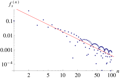
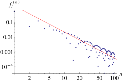
Figure 1: [Left] Small-$g$ expansion coefficients $|f_{s}^{(n)}|$ are plotted to $n$ in log-log scale. [Right] Large-$g$ expansion coefficients $|f_{l}^{(n)}|$ are plotted to $n$ in log-log scale.

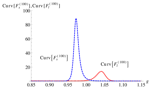
Figure 2: Absolute value of curvature of $F^{(100)}_{s}(g)$ and $F^{(100)}_{l}(g)$ with respect to $g$.

Based on the expansions (4.6), we can construct the interpolating functions in the ways explained in subsection 2.1. We have constructed the several interpolating functions which are listed in (D.1) in Appendix D.1.

We consider the following linear combinations of the interpolating functions by using the functions in (D.1)

$$\hat{G}^{[r,s]}(g)= c_{1}^{[r,s]}F^{(-1)}_{1,1}(g)+c_{2}^{[r,s]}F^{(-1/3)}_{1,1}(g)+c_{3}^{[r,s]}F^{(-1)}_{2,2}(g)+c_{4}^{[r,s]}F^{(-1/3)}_{2,2}(g)\mbox{$$}$$

$$+c_{5}^{[r,s]}F^{(-1/5)}_{2,2}(g)+c_{6}^{[r,s]}F^{(-1)}_{3,3}(g)+c_{7}^{[r,s]}F^{(-1/3)}_{3,3}(g)+c_{8}^{[r,s]}F^{(-1/5)}_{3,3}(g)\mbox{$$}$$

$$+c_{9}^{[r,s]}F^{(-1/7)}_{3,3}(g)+c_{10}^{[r,s]}F^{(-1)}_{4,4}(g)+c_{11}^{[r,s]}F^{(-1/3)}_{4,4}(g)+c_{12}^{[r,s]}F^{(-1/5)}_{4,4}(g)\mbox{$$}$$

$$+c_{13}^{[r,s]}F^{(-1/7)}_{4,4}(g)+c_{14}^{[r,s]}F^{(-1/9)}_{4,4}(g),$$ (4.8)

where

$$\sum_{i=1}^{14}c_{i}^{[r,s]}=1,\qquad c_{i}^{[r,s]}\geq 0.$$ (4.9)

Here $c_{i}^{[r,s]}$ are randomly chosen by using the random number generator in the Mathematica. The superscript $[r,s]$ indicates the $r$-th sample for the $s$-th calculation of correlation coefficients. (We use 10 samples for 1st calculation, 20 samples for 2nd one, 30 samples for 3rd one, 50 samples for 4th one and 100 samples for 5th calculation.) At least these functions match with the small-$g$ and large-$g$ expansions up to

$$F^{(100)}_{s}(g)-\hat{G}^{[r,s]}(g)={\cal O}(g^{2}),\qquad F^{(100)}_{l}(g)-\hat{G}^{[r,s]}(g)={\cal O}(1/g).$$ (4.10)

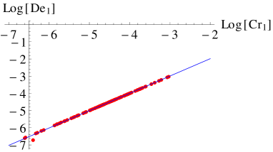
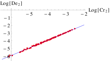
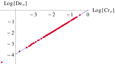
Figure 3: Plots of the $(Cr_{1},De_{1})$, $(Cr_{2},De_{2})$ and $(Cr_{o},De_{o})$ during the fifth computation of the correlation coefficients in case of the true function $F(g)=(1-\frac{g}{5}+g^{2})^{\frac{1}{2}}$. Here the blue line is the regression line.

We check the reliability of the reference quantity $Cr_{1}$ by computing the correlation coefficients between $Cr_{1}$ and $De_{1}$. We compute it five times and the results are

$$\rho^{[1]}_{Cr_{1}De_{1}}=1,\quad\rho^{[2]}_{Cr_{1}De_{1}}=0.999998,\quad\rho^{[3]}_{Cr_{1}De_{1}}=0.999998,\mbox{$$}$$

$$\rho^{[4]}_{Cr_{1}De_{1}}=0.999999,\quad\rho^{[5]}_{Cr_{1}De_{1}}=0.999988,$$ (4.11)

where $\rho^{[i]}_{Cr_{1}De_{1}}$ is the correlation coefficient computed by the $i$-th calculation. The plots of $(Cr_{1},De_{1})$ during the fifth computation are shown in Figure 3. Because these are very close to 1, these are so strong that we can rely on $Cr_{1}$ as a very good reference quantity for selecting a good interpolating function. Of course the results in (4.11) are statistically significant since they are larger than $0.765$.

The correlation coefficients between $Cr_{2}$ and $De_{2}$ are

$$\rho^{[1]}_{Cr_{2}De_{2}}=0.99962083,\quad\rho^{[2]}_{Cr_{2}De_{2}}=0.99949903,\quad\rho^{[3]}_{Cr_{2}De_{2}}=0.99890653,\mbox{$$}$$

$$\rho^{[4]}_{Cr_{2}De_{2}}=0.99916978,\quad\rho^{[5]}_{Cr_{2}De_{2}}=0.999553356,$$ (4.12)

and the ones between $Cr_{o}$ and $De_{o}$ are

$$\rho^{[1]}_{Cr_{o}De_{o}}=0.99995961,\quad\rho^{[2]}_{Cr_{o}De_{o}}=0.99996129,\quad\rho^{[3]}_{Cr_{o}De_{o}}=0.99996000,\mbox{$$}$$

$$\rho^{[4]}_{Cr_{o}De_{o}}=0.99996445,\quad\rho^{[5]}_{Cr_{o}De_{o}}=0.99995738.$$ (4.13)

These quantities are calculated by using the same samples as (4.11). The plots of the $(Cr_{2},De_{2})$ and $(Cr_{o},De_{o})$ during the fifth computation are listed in Figure 3. Since these are also very close to 1, $Cr_{2}$ and $Cr_{o}$ are also good reference quantities.

4.2 Functions where one of small-$g$ or large-$g$ expansions is convergent while the other is asymptotic

4.2.1 $\varphi^{4}$ theory

Let us consider the partition function of the zero-dimensional $\varphi^{4}$ theory,

$$F(g)=\int^{\infty}_{-\infty}d\varphi\,e^{-\frac{\varphi^{2}}{2}-g^{2}\varphi^{4}}.$$ (4.14)

It is well known that the small-$g$ expansion is asymptotic while the large-$g$ expansion is convergent. Interpolating functions for this example have been studied also in section 4.1 of [1].

We assume that we do not know the true function $F(g)$. Suppose that we know only its large-$g$ and small-$g$ expansions up to only 100-th order. The expansions are given by

$$\tilde{F}^{(100)}_{s}(g)=\sum_{k=0}^{100}s_{k}g^{k},\qquad\tilde{F}^{(100)}_{l}(g)=\frac{1}{\sqrt{g}}\sum_{k=0}^{100}l_{k}g^{-k},$$ (4.15)

where the coefficients $s_{k}$ and $l_{k}$ are already known.

We will show $g_{s}^{\ast},g_{l}^{\ast},N_{s}^{\ast}$ and $N_{l}^{\ast}$ which were already given in [1]. According to [1], the small-$g$ expansion was clarified to be an asymptotic expansion, and its related values are

$$g_{s}^{\ast}=0.0680628,\qquad N_{s}^{\ast}=28,$$ (4.16)

where the error is $\epsilon=10^{-7}$. The large-$g$ expansion was estimated to be convergent, and the related quantities are

$$g_{l}^{\ast}=0.1,\qquad N_{l}^{\ast}=100.$$ (4.17)

By taking into account $N_{s}^{\ast}=28$ in the small-$g$ expansion, we need to redefine the expansions by performing the optimal truncation as follows

$$F^{(28)}_{s}(g)=\sum_{k=0}^{28}s_{k}g^{k},\qquad F^{(100)}_{l}(g)=\frac{1}{\sqrt{g}}\sum_{k=0}^{100}l_{k}g^{-k}.$$ (4.18)

We will construct the interpolating functions based on these expansions (4.18). Several interpolating functions are given by eq. (B.1) of [1]. As in (2.13) and (4.8), we consider the interpolating functions, which are linear combinations of the functions in eq. (B.1) of [1] with the randomly generated coefficients, as the samples.

We calculate the correlation coefficients by using the samples. The correlation coefficients between $Cr_{1}$ and $De_{1}$ are

$$\rho^{[1]}_{Cr_{1}De_{1}}=1,\quad\rho^{[2]}_{Cr_{1}De_{1}}=0.999823,\quad\rho^{[3]}_{Cr_{1}De_{1}}=1,\mbox{$$}$$

$$\rho^{[4]}_{Cr_{1}De_{1}}=1,\quad\rho^{[5]}_{Cr_{1}De_{1}}=1.$$ (4.19)

The ones between $Cr_{2}$ and $De_{2}$ are

$$\rho^{[1]}_{Cr_{2}De_{2}}=0.999999,\quad\rho^{[2]}_{Cr_{2}De_{2}}=0.999997,\quad\rho^{[3]}_{Cr_{2}De_{2}}=0.999997,\mbox{$$}$$

$$\rho^{[4]}_{Cr_{2}De_{2}}=0.999997,\quad\rho^{[5]}_{Cr_{2}De_{2}}=0.999998,$$ (4.20)

and the ones between $Cr_{o}$ and $De_{o}$ are

$$\rho^{[1]}_{Cr_{o}De_{o}}=0.999997,\quad\rho^{[2]}_{Cr_{o}De_{o}}=0.999991,\quad\rho^{[3]}_{Cr_{o}De_{o}}=0.999992,\mbox{$$}$$

$$\rho^{[4]}_{Cr_{o}De_{o}}=0.999993,\quad\rho^{[5]}_{Cr_{o}De_{o}}=0.999994.$$ (4.21)

Here (4.20) and (4.21) are computed by using the same samples as (4.19). Because these correlation coefficients are almost 1, all the $Cr_{1}$, $Cr_{2}$ and $Cr_{o}$ work very well as good reference quantities for choosing a good interpolating function.

4.2.2 Average plaquette in the four-dimensional $SU(3)$ pure Yang-Mills theory on the lattice

As a next example, we consider the average plaquette

$$P(\beta)=\Bigl{\langle}1-\frac{1}{3}{\rm Tr}U_{\mathbf{x},\mu}U_{\mathbf{x}+\hat{\mu},\nu}U_{\mathbf{x}+\hat{\nu},\mu}^{\dagger}U_{\mathbf{x},\nu}^{\dagger}\Bigr{\rangle}$$ (4.22)

in the four dimensional $SU(3)$ pure Yang-Mills theory on the lattice. The action of the theory is given by

$$S=\beta\sum_{\mu<\nu}\sum_{\mathbf{x}}\Bigl{[}1-\frac{1}{3}{\rm ReTr}U_{\mathbf{x},\mu}U_{\mathbf{x}+\hat{\mu},\nu}U_{\mathbf{x}+\hat{\nu},\mu}^{\dagger}U_{\mathbf{x},\nu}^{\dagger}\Bigr{]},$$ (4.23)

where $U_{\mathbf{x},\mu}$ is the link variable along the $\mu$-direction at the position $\mathbf{x}$. Here $\hat{\mu}$ denotes the unit vector along the $\mu$-direction. Here the true function for the average plaquette $P(\beta_{i})$ has been obtained by the Monte Carlo simulation in [1]. The interpolating functions for $P(\beta)$ were also studied in [1].

Ref. [9] has given the strong coupling expansion around $\beta=0$,

$$P_{s}^{(15)}(\beta)=\sum_{k=0}^{15}s_{k}\beta^{k},$$ (4.24)

where the coefficients are explicitly described in (4.30) of [1]. The weak coupling expansion around $\beta=\infty$ is given by [10] (see also [11, 12, 13, 14])

$$P_{l}^{(34)}(\beta)=\frac{1}{\beta}\sum_{k=0}^{34}l_{k}\beta^{-k},$$ (4.25)

where the coefficients are listed in (4.32) of [1].

According to the study in [1], the small-$\beta$ expansion is convergent and its related quantities are given by

$$\beta_{s}^{\ast}=3.9,\quad N_{s}^{\ast}=15.$$ (4.26)

On the other hand, the large-$\beta$ expansion turned out to be asymptotic, and the related values were given by

$$\beta_{l}^{\ast}=6.13706,\quad N_{l}^{\ast}=34.$$ (4.27)

Several interpolating functions were already given by eq. (B.6) of [1]. As in (2.13) and (4.8), we consider interpolating functions $\hat{P}^{[r,s]}$, which are the linear combinations of the functions in eq. (B.6) of [1] with randomly generated coefficients, as samples of interpolating functions.

In terms of the true function $P(\beta_{i})$, the sets $(Cr_{1},De_{1})$ $(Cr_{2},De_{2})$ and $(Cr_{o},De_{o})$ are given by

$$De_{1}={\rm Max}\left\{\left|P(\beta_{i})-\hat{P}^{[r,s]}(\beta_{i})\right|;i=1\sim 29\right\},$$ (4.28)

$$De_{2}=\frac{1}{29}\sum_{i=1}^{29}\left|\frac{P(\beta_{i})-\hat{P}^{[r,s]}(\beta_{i})}{P(\beta_{i})}\right|,$$ (4.29)

$$De_{o}=\frac{1}{29}\sum_{i=1}^{29}\left|P(\beta_{i})-\hat{P}^{[r,s]}(\beta_{i})\right|,$$ (4.30)

and

$$Cr_{1}={\rm Max}\left[\left\{\left|\hat{P}^{[r,s]}(\beta)-P_{s}^{(15)}(\beta)\right|;0\leq\beta\leq\beta_{s}^{\ast}\right\}\cup\left\{\left|\hat{P}^{[r,s]}(\beta)-P_{l}^{(34)}(\beta)\right|;\beta_{l}^{\ast}\leq\beta\right\}\right],$$ (4.31)

$$Cr_{2}=\int^{\beta_{s}^{\ast}}_{0}d\beta\left|\frac{\hat{P}^{[r,s]}(\beta)-P_{s}^{(15)}(\beta)}{P_{s}^{(15)}(\beta)}\right|+\int_{\beta_{l}^{\ast}}^{\infty}d\beta\left|\frac{\hat{P}^{[r,s]}(\beta)-P_{l}^{(34)}(\beta)}{P_{l}^{(34)}(\beta)}\right|,$$ (4.32)

$$Cr_{o}=\int^{\beta_{s}^{\ast}}_{0}d\beta\left|\hat{P}^{[r,s]}(\beta)-P_{s}^{(15)}(\beta)\right|+\int_{\beta_{l}^{\ast}}^{\infty}d\beta\left|\hat{P}^{[r,s]}(\beta)-P_{l}^{(34)}(\beta)\right|.$$ (4.33)

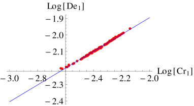
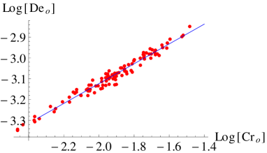
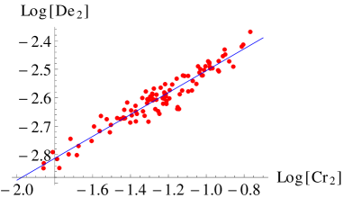
Figure 4: Plots of $(Cr_{1},De_{1})$, $(Cr_{o},De_{o})$ and $(Cr_{2},De_{2})$ during the 5-th calculation of the correlation coefficients in case of the average plaquette in the 4-dimensional $SU(3)$ pure Yang-Mills theory on the lattice. We can see that the correlation between $Cr_{1}$ and $De_{1}$ is the strongest.

Let us check whether $Cr_{1,2,o}$ work well as reference quantities or not by computing the correlation coefficients between $Cr_{j}$ and $De_{j}$ for $j\in\{1,2,o\}$. The correlation coefficients between $Cr_{1}$ and $De_{1}$ are

$$\rho^{[1]}_{Cr_{1}De_{1}}=0.998887,\quad\rho^{[2]}_{Cr_{1}De_{1}}=0.998455,\quad\rho^{[3]}_{Cr_{1}De_{1}}=0.998134,\mbox{$$}$$

$$\rho^{[4]}_{Cr_{1}De_{1}}=0.999318,\quad\rho^{[5]}_{Cr_{1}De_{1}}=0.998927.$$ (4.34)

The ones between $Cr_{o}$ and $De_{o}$ are

$$\rho^{[1]}_{Cr_{o}De_{o}}=0.990178,\quad\rho^{[2]}_{Cr_{o}De_{o}}=0.987834,\quad\rho^{[3]}_{Cr_{o}De_{o}}=0.975302,\mbox{$$}$$

$$\rho^{[4]}_{Cr_{o}De_{o}}=0.982322,\quad\rho^{[5]}_{Cr_{o}De_{o}}=0.982845,$$ (4.35)

and the correlation coefficients between $Cr_{2}$ and $De_{2}$ are

$$\rho^{[1]}_{Cr_{2}De_{2}}=0.98446,\quad\rho^{[2]}_{Cr_{2}De_{2}}=0.968163,\quad\rho^{[3]}_{Cr_{2}De_{2}}=0.938417,\mbox{$$}$$

$$\rho^{[4]}_{Cr_{2}De_{2}}=0.959227,\quad\rho^{[5]}_{Cr_{2}De_{2}}=0.956638,$$ (4.36)

where (4.35) and (4.36) are computed by using the same samples as (4.34). These are of course statistically significant, and these are very close to 1. So $Cr_{1,2,o}$ are sufficiently good reference quantities for selecting a good interpolating function. By comparing (4.34) with (4.35) and (4.36), $Cr_{1}$ turns out to be the best reference quantity because of the strongest correlation to the actual degree of deviation. (We can also see it by comparing the plots in Figs. 4)

4.3 Functions where the both expansions are asymptotic

4.3.1 $F(g)=e^{\frac{1}{g^{4}}}e^{g^{4}}K_{\frac{1}{4}}\left(\frac{1}{g^{4}}\right)K_{\frac{1}{4}}(g^{4})$

We will consider the example with following true function

$$F(g)=e^{\frac{1}{g^{4}}}e^{g^{4}}K_{\frac{1}{4}}\left(\frac{1}{g^{4}}\right)K_{\frac{1}{4}}(g^{4}),$$ (4.37)

where $K_{\frac{1}{4}}(x)$ is the modified Bessel function of the second kind with order $\frac{1}{4}$. The small-$g$ and large-$g$ expansions of the function take following forms

$$F^{(N_{s})}_{s}(g)= g\sum_{k=0}^{{\rm floor}(\frac{N_{s}}{2})}s_{2k}g^{2k}=g\sum_{k=0}^{{\rm floor}(\frac{N_{s}}{4})}s_{4k}g^{4k}+g\sum_{k=0}^{{\rm floor}(\frac{N_{s}}{4})}s_{4k+2}g^{4k+2},$$ (4.38)

$$F^{(N_{l})}_{l}(g)= \frac{1}{g}\sum_{k=0}^{{\rm floor}(\frac{N_{l}}{2})}l_{2k}g^{-2k}=\frac{1}{g}\sum_{k=0}^{{\rm floor}(\frac{N_{l}}{4})}l_{4k}g^{-4k}+\frac{1}{g}\sum_{k=0}^{{\rm floor}(\frac{N_{l}}{4})}l_{4k+2}g^{-4k-2}.$$ (4.39)

Here ${\rm floor}(x)=\max\{n\in{\mathbb{Z}};n\leq x\}$ which is called as the floor function. The $F(g)$ is a symmetric function under the exchange of $g$ and $1/g$. By extrapolating the data of $\left|\frac{s_{2k+2}}{s_{2k}}\right|$ in [Top Left] of Figs. 5, the small-$g$ expansion turns out to be asymptotic since the ratio diverges in large $k$. Analogously we can see that the large-$g$ expansion is also asymptotic.

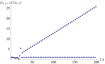
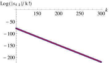
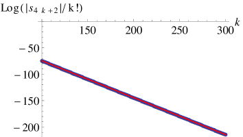
Figure 5: [Top Left] $|s_{2k+2}|/|s_{2k}|$ v.s $k$ [Top Right] $\log(|s_{4k}/k!|)$ v.s $k$ [Bottom] $\log(|s_{4k+2}/k!|)$ v.s $k$.

We observe that $\left|\frac{s_{4k+4}}{s_{4k}}\right|$, $\left|\frac{s_{4k+6}}{s_{4k+2}}\right|$, $\left|\frac{l_{4k+4}}{l_{4k}}\right|$ and $\left|\frac{l_{4k+6}}{l_{4k+2}}\right|$ behave as linear in $k$, so we put ansatz

$$s_{4k}\sim c_{1}A_{1}^{k}k!,\qquad s_{4k+2}\sim c_{2}A_{2}^{k}k!,\qquad l_{4k}\sim d_{1}B_{1}^{k}k!,\qquad l_{4k+2}\sim d_{2}B_{2}^{k}k!,$$ (4.40)

in large $k$. By fitting the log-plots as in [Top Right] and [Bottom] of Figs. 5, we obtain

$$c_{1}=d_{1}=0.00027207,\quad A_{1}=B_{1}=0.494761,\qquad$$

$$c_{2}=d_{2}=0.00853819,\quad A_{2}=B_{2}=0.497397.$$ (4.41)

Because of $A_{1}\sim B_{1}\sim A_{2}\sim B_{2}\sim\frac{1}{2}$, large order terms in the small-$g$ expansion should be

$$\pm g(c_{1}-c_{2}g^{2})\left(\frac{1}{2}\right)^{k}k!g^{4k}$$ (4.42)

where $k\gg 1$. The relative minus sign inside $(c_{1}-c_{2}g^{2})$ is required because of our observation that $s_{4k}\times s_{4k+2}<0$ upto $k=100$. We expect that the optimal truncation will be implemented at order less than $100$. Based on (4.42), by following the procedure in Appendix B.1, we can obtain $N_{s}^{\ast}$ as well as $g_{s}^{\ast}$. According to the procedure,

$$N_{s}^{\ast}=4\left|\frac{1}{A{g_{s}^{\ast}}^{4}}\right|.$$ (4.43)

$g_{s}^{\ast}$ is given by the solution of the following equation

$$\log\epsilon=\log g_{s}^{\ast}+\log|c_{1}-c_{2}{g_{s}^{\ast}}^{2}|-\frac{2}{{g_{s}^{\ast}}^{4}}.$$ (4.44)

By solving the above (here we set $\epsilon=10^{-7}$), we obtain

$$g_{s}^{\ast}=0.6676,\quad N_{s}^{\ast}=40.$$ (4.45)

Also in the large-$g$ expansion, by following the analogous procedure, we obtain

$$g_{l}^{\ast}=1.4979,\quad N_{l}^{\ast}=40.$$ (4.46)

Based on the expansions $F^{(N_{s}^{\ast})}_{s}(g),F^{(N_{l}^{\ast})}_{l}(g)$ with $N^{\ast}_{s}=N_{l}^{\ast}=40$, we construct the interpolating functions $F_{m,n}^{(\alpha)}$ as

$$F_{m,n}^{(\alpha)}(g)=\frac{\sqrt{\pi}\Gamma(\frac{1}{4})}{2^{\frac{5}{4}}}g\left(\frac{1+\sum_{k=1}^{p}c_{k}g^{2k}}{1+\sum_{k=1}^{q}d_{k}g^{2k}}\right)^{\alpha},$$ (4.47)

where

$$p=\frac{1}{2}\left(\frac{1}{2}m+\frac{1}{2}n+1-\frac{1}{\alpha}\right),\quad q=\frac{1}{2}\left(\frac{1}{2}m+\frac{1}{2}n+1+\frac{1}{\alpha}\right),$$ (4.48)

$$\left|\frac{2}{m+n+2}\right|\leq\left|\alpha\right|,\qquad\alpha=\left\{\begin{matrix}\frac{1}{2\ell+1}&{\rm for}\quad&\frac{1}{2}(m+n):{\rm even}\\ \frac{1}{2\ell}&{\rm for}\quad&\frac{1}{2}(m+n):{\rm odd}\end{matrix}\right.,\qquad\ell\in\mathbb{Z}.$$ (4.49)

Explicit forms of these are described in (D.2) in the Appendix. D.2.

As in (2.13) and (4.8), we consider randomly generated linear combinations of the functions (D.2) as the samples of the interpolating functions.

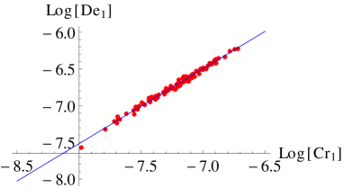
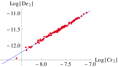
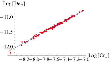
Figure 6: Plots of the $(Cr_{1},De_{1})$, $(Cr_{2},De_{2})$ and $(Cr_{o},De_{o})$ during the 5-th calculation of the correlation coefficients in case of the $F(g)=e^{\frac{1}{g^{4}}}e^{g^{4}}K_{\frac{1}{4}}(\frac{1}{g^{4}})K_{\frac{1}{4}}(g^{4})$

We check the reference quantities by computing the correlation coefficients. The correlation coefficients between $Cr_{1}$ and $De_{1}$ are

$$\rho^{[1]}_{Cr_{1}De_{1}}=0.98965,\quad\rho^{[2]}_{Cr_{1}De_{1}}=0.992231,\quad\rho^{[3]}_{Cr_{1}De_{1}}=0.994823,\mbox{$$}$$

$$\rho^{[4]}_{Cr_{1}De_{1}}=0.991528,\quad\rho^{[5]}_{Cr_{1}De_{1}}=0.994911.$$ (4.50)

The ones between $Cr_{2}$ and $De_{2}$ are

$$\rho^{[1]}_{Cr_{2}De_{2}}=0.996086,\quad\rho^{[2]}_{Cr_{2}De_{2}}=0.996022,\quad\rho^{[3]}_{Cr_{2}De_{2}}=0.996846,\mbox{$$}$$

$$\rho^{[4]}_{Cr_{2}De_{2}}=0.995829,\quad\rho^{[5]}_{Cr_{2}De_{2}}=0.996668,$$ (4.51)

and the ones between $Cr_{o}$ and $De_{o}$ are

$$\rho^{[1]}_{Cr_{o}De_{o}}=0.996176,\quad\rho^{[2]}_{Cr_{o}De_{o}}=0.99628,\quad\rho^{[3]}_{Cr_{o}De_{o}}=0.996872,\mbox{$$}$$

$$\rho^{[4]}_{Cr_{o}De_{o}}=0.995994,\quad\rho^{[5]}_{Cr_{o}De_{o}}=0.996741.$$ (4.52)

In the computation (4.51) and (4.52), we use the same samples as (4.50). Because these are exceeding 0.99 (of course statistically significant), we can take all $Cr_{1},Cr_{2}$ and $Cr_{o}$ as good reference quantities for selecting a good interpolating function. In this case, $Cr_{2,o}$ are slightly better than $Cr_{1}$ but the differences are not so significant according to the comparison between their plots in Figure 6.

4.4 Functions with sharp peak outside the reliable domain

So far we have checked $Cr_{1}$, $Cr_{2}$ and $Cr_{o}$ for the functions which do not have the sharp peak outside the reliable domain (see Figs. 7). For such functions, all $Cr_{1,2,o}$ seem to be good reference quantities, and $Cr_{1}$ seems to be the best.

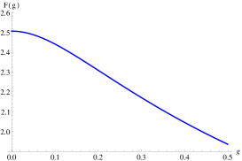
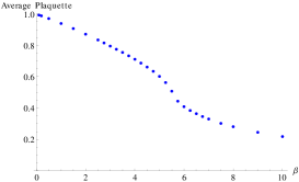
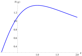
Figure 7: (a) Plot of the function $F(g)=(1-\frac{g}{5}+g^{2})^{\frac{1}{2}}$ to $g$, (b) Plot of $F(g)=\int^{\infty}_{-\infty}d\varphi e^{-\frac{\varphi^{2}}{2}-g^{2}\varphi^{4}}$ to $g$, (c) Plots of Average plaquette in the $SU(3)$ pure Yang-Mills theory on the lattice to $\beta$, (d) Plot of the function $F(g)=e^{\frac{1}{g^{4}}}e^{g^{4}}K_{\frac{1}{4}}(\frac{1}{g^{4}})K_{\frac{1}{4}}(g^{4})$ to $g$.

In this subsection, we will investigate the reference quantities for the functions with sharp peak outside the reliable domain. We will check whether they work well or not even in the presence of the sharp peak, by calculating the correlation coefficients. In this subsection, as the functions with sharp peak, we use the specific heat functions in the two dimensional Ising model with lattice size $L=5,8,\infty$. By Figure 8, we can see that the functions with $L=5,8$ have sharp peak moreover the $L=\infty$ function has the singular point which is regarded as the phase transition point.

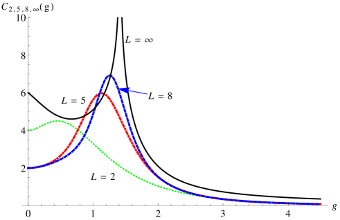
Figure 8: We plot the specific heat in the 2 dimensional Ising model against $g$ for various lattice sizes $L=2,5,8,\infty$. In cases of $L=5,8$, the peaks locate outside the reliable domain, where $g_{s}^{\ast}=0.4$, $g_{l}^{\ast}=3.8$ in $L=5$, and $g_{s}^{\ast}=0.4$, $g_{l}^{\ast}=3.7$ in $L=8$ case.

Concise review of the specific heat in the two-dimensional Ising model

We will consider the two-dimensional Ising model on the $L\times L$ square lattice with periodic boundary condition. The detailed explanation is in section 4.2 of [1]. The Hamiltonian of the Ising model is described as

$$H=-J\sum_{\langle\mathbf{x},\mathbf{y}\rangle}\sigma_{\mathbf{x}}\sigma_{\mathbf{y}}.$$ (4.53)

Here $\mathbf{x}$ and $\mathbf{y}$ denote the locations of the lattice sites taking integer value. The notation $\langle\mathbf{x},\mathbf{y}\rangle$ indicates the sum over pairs of adjacent spins. $\sigma_{\mathbf{x}}$ describes the spin variable at $\mathbf{x}$ taking $\sigma_{\mathbf{x}}=\pm 1$. $J$ denotes the exchange energy (coupling constant) between the nearest neighbor spins. The partition function of the model with respect to the temperature $T$ is

$$Z_{L}(K)=\sum_{\{\rm state\}}e^{-\frac{1}{T}H}=\sum_{\{\rm state\}}e^{K\sum_{(\mathbf{x},\mathbf{y})}\sigma_{\mathbf{x}}\sigma_{\mathbf{y}}},\quad{\rm with}\ K=\frac{J}{T},$$ (4.54)

and it has been calculated exactly in [16],

$$Z_{L}(K)=\frac{1}{2}\left(S_{11}(K)+2S_{10}(K)-S_{00}(K)\right),\mbox{$$}$$

$$S_{\sigma_{1}\sigma_{2}}(K)=2^{L^{2}}\prod_{p,q=0}^{L-1}\Bigl{[}\cosh^{2}{(2K)}-\sinh{(2K)}\Bigl{(}\cos{\frac{(2p+\sigma_{1})\pi}{L}}+\cos{\frac{(2q+\sigma_{2})\pi}{L}}\Bigr{)}\Bigr{]}^{\frac{1}{2}}.\mbox{$$}$$

Based on the partition function, we introduce the following quantity

$$C_{L}(K)=\frac{1}{L^{2}}\frac{\partial^{2}}{\partial K^{2}}\log{Z_{L}(K)}.$$ (4.56)

In terms of the $C_{L}(K)$, the specific heat can be given by $K^{2}C_{L}(K)$. For considering the power series form (2.1) of both the high and low temperature expansion, we introduce the parameter $g$ by

$$e^{2K}=1+g.$$ (4.57)

Then the power series expansion of $g$ around $g=0$ corresponds to the high temperature expansion while the $1/g$ expansion around the $g=\infty$ corresponds to the low temperature expansion.

4.4.1 $5\times 5$ lattice

For $L=5$, the specific heat $C_{5}(g)$ is obtained by substituting $L=5$ into (4.56). The true function $C_{5}(g)$ has a sharp peak as shown in Figure 8. We will pay attention to how the peak affects the correlation coefficients $\rho_{Cr_{1}De_{1}}$, $\rho_{Cr_{2}De_{2}}$ and $\rho_{Cr_{o}De_{o}}$.

We assume that we know only the small-$g$ and large-$g$ expansions up to $N_{s}=N_{l}=50$-th order,

$$C_{5s}^{(50)}(g)=\sum_{k=0}^{50}s_{k}g^{k},\qquad C_{5l}^{(50)}(g)=g^{-4}\sum_{k=0}^{50}l_{k}g^{-k}.$$ (4.58)

Their leading order terms are

$$C_{5s}^{(50)}(g)= 2+\frac{5g^{2}}{2}-\frac{3g^{3}}{2}+\frac{17g^{4}}{8}+\mathcal{O}\left(g^{5}\right),\mbox{$$}$$

$$C_{5l}^{(50)}(g)= g^{-4}\left(64-256g^{-1}+928g^{-2}-3008g^{-3}+9440g^{-4}+\mathcal{O}(g^{-5})\right).$$ (4.59)

By the extrapolation in [1], we can read

$$N_{s}^{\ast}=50,\quad g_{s}^{\ast}=0.4,\quad N_{l}^{\ast}=50,\quad g_{l}^{\ast}=3.8,$$ (4.60)

and it turned out that both the expansions are convergent. As shown in Figure 8, the sharp peak locates outside the reliable domain, $g_{s}^{\ast}<g<g_{l}^{\ast}$. Because of $N_{s}^{\ast}=N_{s},N_{l}^{\ast}=N_{l}$, we can use (4.58) directly to make the interpolating functions. Several interpolating functions have been given in eq. (B.3) of [1] already. As in (2.13) and (4.8), we consider randomly generated linear combinations of functions in eq. (B.3) of [1] as the samples of interpolating functions. By using the samples, we calculate the correlation coefficients. The correlation coefficients are

$$\rho^{[1]}_{Cr_{1}De_{1}}=0.8031<\rho^{[1]}_{Cr_{o}De_{o}}=0.88367308<\rho^{[1]}_{Cr_{2}De_{2}}=0.97453243,\mbox{$$}$$

$$\rho^{[2]}_{Cr_{1}De_{1}}=0.632352<\rho^{[2]}_{Cr_{o}De_{o}}=0.68630313<\rho^{[2]}_{Cr_{2}De_{2}}=0.90483010,\mbox{$$}$$

$$\rho^{[3]}_{Cr_{1}De_{1}}=0.695725<\rho^{[3]}_{Cr_{o}De_{o}}=0.78550976<\rho^{[3]}_{Cr_{2}De_{2}}=0.93317359,\mbox{$$}$$

$$\rho^{[4]}_{Cr_{1}De_{1}}=0.609671<\rho^{[4]}_{Cr_{o}De_{o}}=0.74064316<\rho^{[4]}_{Cr_{2}De_{2}}=0.93436356,\mbox{$$}$$

$$\rho^{[5]}_{Cr_{1}De_{1}}=0.666964<\rho^{[5]}_{Cr_{o}De_{o}}=0.76862717<\rho^{[5]}_{Cr_{2}De_{2}}=0.93445856.$$ (4.61)

We should note that the correlation coefficients $\rho_{Cr_{1}De_{1}}$ and $\rho_{Cr_{o}De_{o}}$ become weak, while the correlations between $Cr_{2}$ and $De_{2}$ are still strong (bigger than $0.9$). So the reference quantities $Cr_{1,o}$ become useless by the appearance of the sharp peak outside the reliable domain, while $Cr_{2}$ is still useful. We can compare between them by using the plots Figure 9 also.

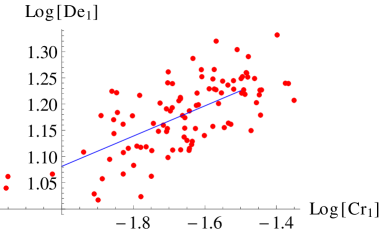
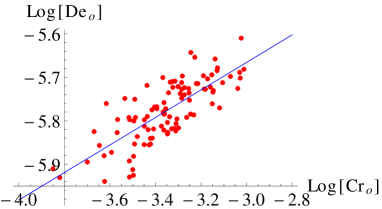
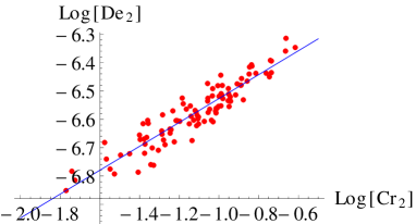
Figure 9: Plots of $(Cr_{1},De_{1})$, $(Cr_{o},De_{o})$ and $(Cr_{2},De_{2})$ during the 5-th computation of the correlation coefficients in case of the $L=5$ Ising model. We can see that the set $(Cr_{2},De_{2})$ have much stronger correlation than the others, where the plots of $(Cr_{o},De_{o})$ and $(Cr_{1},De_{1})$ are more scattered.

One might wonder how we can notice the presence of the sharp peak without knowing the true function. Even without knowing the true function, by plotting an interpolating function, we can guess the presence of the sharp peak. If a true function has a sharp peak, its interpolating function tends to have a sharp peak as shown in Figure 10. This study instructs that if there is a sharp peak in an interpolating function, we should start to use $Cr_{2}$ only.

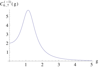
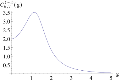
Figure 10: [Left] Plot of $C_{6,7}^{(-1)}(g)$ to $g$ in the $L=5$ case. [Right] Plot of $C_{6,7}^{(-1)}(g)$ with respect to $g$ in the $L=8$ case. We can see that interpolating functions also have sharp peaks.

4.4.2 $8\times 8$ lattice

The function $C_{8}(g)$ for $L=8$ also has a sharp peak as shown in Figure 8. Even if we do not know about the true function $C_{8}(g)$, we can deduce the presence of the peak by plotting an interpolating function as shown in Figure 10.

Also in this example, we assume that we know only the small-$g$ and large-$g$ expansions upto $N_{s}=N_{l}=50$-th order,

$$C_{8s}^{(50)}(g)=\sum_{k=0}^{50}s_{k}g^{k},\qquad C_{8l}^{(50)}(g)=g^{-4}\sum_{k=0}^{50}l_{k}g^{-k},$$ (4.62)

where their leading order terms are

$$C_{8s}^{(50)}(g)= 2+\frac{5g^{2}}{2}-\frac{5g^{3}}{2}+\frac{29g^{4}}{8}+\mathcal{O}(g^{5}),\mbox{$$}$$

$$C_{8l}^{(50)}(g)= g^{-4}\left(64-256g^{-1}+928g^{-2}-3008g^{-3}+9440g^{-4}+\mathcal{O}(g^{-5})\right),$$ (4.63)

respectively. By the study in [1], it has been known that

$$N_{s}^{\ast}=50,\quad g_{s}^{\ast}=0.4,\quad N_{l}^{\ast}=50,\quad g_{l}^{\ast}=3.7,$$ (4.64)

and that both the expansions are convergent. We can see that the peak locates outside the reliable domain as shown by Figure 8. As in the previous case, because of $N_{s}^{\ast}=N_{s},N_{l}^{\ast}=N_{l}$, we can use (4.62) directly to make the interpolating functions. Several interpolating functions were already given in eq. (B.4) of [1]. As in (2.13) and (4.8), we generate interpolating functions randomly as the samples by linear combinations of the functions in eq. (B.4) of [1]. We compute the correlation coefficients by using the samples. The correlation coefficients are

$$\rho^{[1]}_{Cr_{1}De_{1}}=0.611783<\rho^{[1]}_{Cr_{o}De_{o}}=0.74837673<\rho^{[1]}_{Cr_{2}De_{2}}=0.86202835,\mbox{$$}$$

$$\rho^{[2]}_{Cr_{1}De_{1}}=0.732422<\rho^{[2]}_{Cr_{o}De_{o}}=0.89045374<\rho^{[2]}_{Cr_{2}De_{2}}=0.95196590,\mbox{$$}$$

$$\rho^{[3]}_{Cr_{1}De_{1}}=0.743958<\rho^{[3]}_{Cr_{o}De_{o}}=0.87655349<\rho^{[3]}_{Cr_{2}De_{2}}=0.95651297,\mbox{$$}$$

$$\rho^{[4]}_{Cr_{1}De_{1}}=0.66496<\rho^{[4]}_{Cr_{o}De_{o}}=0.85658632<\rho^{[4]}_{Cr_{2}De_{2}}=0.95161652,\mbox{$$}$$

$$\rho^{[5]}_{Cr_{1}De_{1}}=0.677466<\rho^{[5]}_{Cr_{o}De_{o}}=0.85909180<\rho^{[5]}_{Cr_{2}De_{2}}=0.94872463.$$ (4.65)

Also in the $L=8$ case, $\rho_{Cr_{1}De_{1}}$ and $\rho_{Cr_{o}De_{o}}$ become weak by the presence of sharp peak. On the other hand the correlations between $Cr_{2}$ and $De_{2}$ are still strong, bigger than $0.9$.

4.4.3 Infinite lattice

In the $L=\infty$ case, the true function has singularity and there is the phase transition. $Cr_{1}$ is obviously no longer useful in this case, then we will focus only on whether $Cr_{2,o}$ can be good reference quantities or not even in the presence of the singularity.

The true function for the specific heat in the $L=\infty$ case is given by

$$C_{\infty}(g) = \frac{16(g+1)}{\pi g(g+2)}\Biggl{[}K\left(\frac{4g(g+1)(g+2)}{\left(g^{2}+2g+2\right)^{2}}\right)-E\left(\frac{4g(g+1)(g+2)}{\left(g^{2}+2g+2\right)^{2}}\right)\mbox{$$}$$ (4.67)

$$-\left(\frac{2(g+1)}{(g+1)^{2}+1}\right)^{2}\left\{\frac{g^{4}+4g^{3}-8g-4}{\left(g^{2}+2g+2\right)^{2}}K\left(\frac{4g(g+1)(g+2)}{\left(g^{2}+2g+2\right)^{2}}\right)+\frac{\pi}{2}\right\}\Biggr{]},$$

where $K(z)$ and $E(z)$ are

$$K(z)=\int_{0}^{\pi/2}dt(1-z\sin^{2}{t})^{-1/2},$$

$$E(z)=\int_{0}^{\pi/2}dt(1-z\sin^{2}{t})^{1/2}.$$

As in the previous cases, we will assume that we know only the small-$g$ and large-$g$ expansions upto $N_{s}=N_{l}=50$-th order,

$$C_{\infty s}^{(50)}(g)=\sum_{k=0}^{50}s_{k}g^{k},\qquad C_{\infty l}^{(50)}(g)=g^{-2}\sum_{k=0}^{50}l_{k}g^{-k},$$ (4.68)

their leading order terms are

$$C_{\infty s}^{(50)}(g)= 6-\frac{11g}{4}-\frac{15g^{2}}{4}+\frac{3265g^{3}}{256}-\frac{651g^{4}}{64}+\mathcal{O}(g^{5}),\mbox{$$}$$

$$C_{\infty l}^{(50)}(g)= g^{-2}\left(16-72g^{-1}+164g^{-2}+15g^{-3}-\frac{3087}{4}g^{-4}+\mathcal{O}(g^{-5})\right),$$ (4.69)

respectively. By the extrapolation in [1], we obtain

$$N_{s}^{\ast}=50,\quad g_{s}^{\ast}=1,\quad N_{l}^{\ast}=50,\quad g_{l}^{\ast}=2,$$ (4.70)

and we can see that both the expansions are convergent. So we can use (4.68) directly to make the interpolating functions. Several interpolating functions are already given by eq. (B.5) of [1]. We generate interpolating functions randomly by the linear combinations of functions in eq. (B.5) of [1] as in the previous cases. By using the generated functions as the samples, we check the reference quanities $Cr_{2,o}$ by calculating the correlation coefficients. The correlation coefficients between $Cr_{2}$ and $De_{2}$ are

$$\rho^{[1]}_{Cr_{2}De_{2}}=0.9889143983,\quad\rho^{[2]}_{Cr_{2}De_{2}}=0.9857282660,\quad\rho^{[3]}_{Cr_{2}De_{2}}=0.9746687539,\mbox{$$}$$

$$\rho^{[4]}_{Cr_{2}De_{2}}=0.9835468034,\quad\rho^{[5]}_{Cr_{2}De_{2}}=0.9745817796.$$ (4.71)

Even in the presence of the singularity, $Cr_{2}$ has strong correlation with $De_{2}$. Hence the $Cr_{2}$ can be a reliable reference.

The correlation coefficients between $Cr_{o}$ and $De_{o}$ are also strong,

$$\rho^{[1]}_{Cr_{o}De_{o}}=0.970161493,\quad\rho^{[2]}_{Cr_{o}De_{o}}=0.973184305,\quad\rho^{[3]}_{Cr_{o}De_{o}}=0.986896467,\mbox{$$}$$

$$\rho^{[4]}_{Cr_{o}De_{o}}=0.9928459634,\quad\rho^{[5]}_{Cr_{o}De_{o}}=0.9903143989.$$ (4.72)

They are even stronger than the ones between $Cr_{2}$ and $De_{2}$. But unlike the $L=5,8$ cases, $\rho_{Cr_{2}De_{2}}$ are also strong enough and there are not so much differences between $\rho_{Cr_{2}De_{2}}$ and $\rho_{Cr_{o}De_{o}}$. Also from the plots in Fig. 11, we can see that there are not so much differences between $\rho_{Cr_{2}De_{2}}$ and $\rho_{Cr_{o}De_{o}}$.

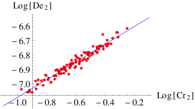
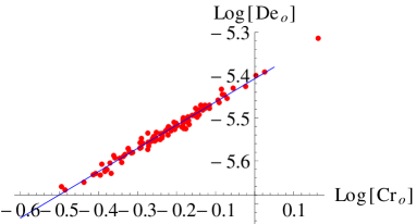
Figure 11: Plots of $(Cr_{2},De_{2})$ and $(Cr_{o},De_{o})$ during the fifth calculation of the correlation coefficient in case of the $L=\infty$ Ising model.

5 Conclusion $\&$ discussion

We suggested the quantities $Cr_{1,2,o}$ given in (3.4), (3.5) and (3.6) as reference quantities for choosing a good interpolating function. To check whether they are reliable reference quantities or not, we calculated correlation coefficients between $Cr_{j}$ and $De_{j}$ for $j\in\{1,2,o\}$ for several examples. Here $De_{1,2,o}$ are given by (3.1), (3.2) and (3.3). We observed

1. For functions without sharp peak outside the reliable domain, all $Cr_{1,2,o}$ can be good reference quantities for choosing a good interpolating function. Among them $Cr_{1}$ seems to be the best reference quantity. This comes from the observations in (4.11)$\sim$(4.13), (4.19)$\sim$(4.21), (4.34)$\sim$(4.36) and (4.50)$\sim$(4.52).

2. For functions with sharp peak outside the reliable domain, only $Cr_{2}$ can be reliable. This comes from the observations in (4.61), (4.65) and (4.71).

Usually the sharp peak in the true function can be found by plotting the interpolating functions. This observation indicates that the combination of $Cr_{1}$ and $Cr_{2}$ works as the best reference for selecting a good interpolating function. It is also convenient to use $Cr_{2}$ only, because only $Cr_{2}$ has universal usage independent of functions.

The analysis in this paper requires the large order expansions which was true for the examples we considered. But in many cases, we may not have large order expansions. So, it is important to establish a way to estimate $g_{s}^{\ast},g_{l}^{\ast},N_{s}^{\ast}$ and $N_{l}^{\ast}$ also for the cases where we have limited number of expansions.

Acknowledgment

We are grateful to Masazumi Honda and Ashoke Sen for their collaboration at the early stage of this project. Especially, we would like to thank Ashoke Sen for suggesting the author to write down this paper and kindly reading the manuscript carefully. We thank Abhishek Chowdhury, Yoshinori Honma, Swapnamay Mondal, Satchitananda Naik, Kenji Nishiwaki, Kenji Ogawa, Tetsuya Onogi, Roji Pius and Koji Tsumura for valuable discussions and comments. In particular, we acknowledge Roji Pius for reading the manuscript. T.T would like to express the gratitude for the hospitality offered by NTU (particularly Pei-Ming Ho and Heng-Yu Chen and related secretaries), Weizmann institute (particularly Ofer Aharony and related secretaries), ICTP (particularly Kumar Narain and related secretaries) during his stay. He is also thankful to the kind support provided by the Strings 2014 organizers. Finally he wishes to acknowledge the kind support provided by the Indian people.

Appendix A Insufficiency of the criterion given in [1]

As discussed in subsection 2.2, there are uncountably infinite number of interpolating functions, because a linear combination of interpolating functions is also an interpolating function again. So it is important to establish a criterion for selecting a good interpolating function. In [1], the authors proposed such a criterion, but we will argue that their criterion is insufficient.

Let us start by a brief review of the analysis given in [1]. First of all, they picked up one subset from infinite number of interpolating functions $G(g)$ where $g$ is the parameter. We should note that this subset has no particular significance compared to any other possible subsets. Within the selected subset they observed the following matching

(the function $$G(g) I_{s}[G(g)]+I_{l}[G(g)]$$ with the smallest in the subset)

$$= \text{(the function $G(g)$ with the smallest $\Lambda^{-1}\int_{0}^{\Lambda}dg\left|\frac{G(g)-F(g)}{F(g)}\right|$ in the subset)},$$ (A.1)

here $\Lambda^{-1}\int_{0}^{\Lambda}dg\left|\frac{G(g)-F(g)}{F(g)}\right|$ measures deviation between $G(g)$ and the true function $F(g)$. $I_{s}[G(g)],I_{l}[G(g)]$ are defined in (3.1) of [1],

$$I_{s}[G]=\int^{g^{\ast}_{s}}_{0}dg\left|G(g)-F^{(N_{s}^{\ast})}_{s}(g)\right|,\quad I_{l}[G]=\int_{g^{\ast}_{l}}^{\Lambda}dg\left|G(g)-F^{(N_{l}^{\ast})}_{l}(g)\right|$$ (A.2)

where $F_{s}^{(N_{s}^{\ast})}$ and $F_{l}^{(N_{l}^{\ast})}$ are the small-$g$ and large-$g$ expansions up to order $N_{s}^{\ast}$ and $N_{l}^{\ast}$ respectively. Here the validity of the expansions $F_{s}^{(N_{s}^{\ast})}$ and $F_{l}^{(N_{l}^{\ast})}$ are limited to the domains $0<g<g_{s}^{\ast}$ and $g_{l}^{\ast}<g$ respectively. (In our discussions, we denoted $I_{s}+I_{l}$ by $Cr$ and $\Lambda^{-1}\int_{0}^{\Lambda}dg\left|\frac{G(g)-F(g)}{F(g)}\right|$ by $De$.) Based on the above observation (A.1) which is true within the selected subset, they asserted that the best interpolating function has the minimum value for $I_{s}[G]+I_{l}[G]$. But we should remember that the notion of the criterion should be independent of the choice of subset. By constructing an explicit example, we will show in the following subsection that it is possible to choose another subset where the observation (A.1) is not valid. This means that their criterion in [1] is insufficient as a universal criterion, which should be independent of the choice of the subset.

A.1 A counter example

Let us re-examine the case of the two-dimensional Ising model with lattice size $L=2$ considered in subsubsection 4.2.1 of [1]. There they tried to find interpolating function for the specific heat $C_{2}(g)$. Here the parameter $g=e^{2J/T}-1$ where $J$ is the coupling constant of Ising model and $T$ is the temperature. They computed $De=\Lambda^{-1}\int dg\left|\frac{C_{m,n}^{\alpha}-C_{2}}{C_{2}}\right|$ and $Cr=I_{s}+I_{l}$ for a class of interpolating functions $C_{m,n}^{(\alpha)}$, which are listed in Table 1. For this set of interpolating functions given in the Table 1, the observation (A.1) is true.

	$\Lambda^{-1}\int dg\bigl{|}\frac{C_{m,n}^{(\alpha)}-C_{2}}{C_{2}}\bigr{|}$	$I_{s}[C_{m,n}^{(\alpha)}]$	$I_{l}[C_{m,n}^{(\alpha)}]$	$I_{s}+I_{l}$
$C_{1,1}^{(-4)}$	0.00224809	0.0912750	0.102638	0.193913
$C_{1,1}^{(-4/3)}$	0.000817041	0.0617656	0.0193989	0.0811645
$C_{1,2}^{(-2)}$	0.00100228	0.0751219	0.0466568	0.121779
$C_{1,2}^{(-1)}$	0.000286070	0.058021	0.00257514	0.0605961
$C_{2,2}^{(-4)}$	0.000173889	0.00768450	0.00852503	0.0162095
$C_{2,3}^{(-2)}$	0.000158806	0.00224879	0.00550386	0.00775265
$C_{3,2}^{(-2)}$	0.000322997	0.00658097	0.0116865	0.0182674
$C_{3,4}^{(-1)}$	0.0000147709	0.000148814	0.000258785	0.000407598
$C_{4,3}^{(-2)}$	0.000168121	0.00345741	0.00565649	0.0091139
$C_{4,3}^{(-1)}$	0.0000651441	0.00156065	0.00170668	0.00326733
$C_{5,4}^{(-1)}$	0.0000207392	0.000525855	0.000327812	0.000853666
$C_{6,5}^{(-1)}$	0.0000119340	0.000174690	0.000192164	0.000366854
$\bf C_{7,6}^{(-1)}$	$\bf 1.22853\times 10^{-6}$	$\bf 3.39663\times 10^{-6}$	$\bf 0.0000523107$	0.0000557073
$C_{6,7}^{(-1)}$	0.0000128648	0.000129274	0.0000598797	0.000189154

Table 1: $Cr$ and $De$ in the original subset in [1]

	$\Lambda^{-1}\int dg\bigl{|}\frac{C_{m,n}^{(\alpha)}-C_{2}}{C_{2}}\bigr{|}$	$I_{s}[C_{m,n}^{(\alpha)}]$	$I_{l}[C_{m,n}^{(\alpha)}]$	$I_{s}+I_{l}$
$C_{1,1}^{(-4)}$	0.00224809	0.0912750	0.102638	0.193913
$C_{1,1}^{(-4/3)}$	0.000817041	0.0617656	0.0193989	0.0811645
$C_{1,2}^{(-2)}$	0.00100228	0.0751219	0.0466568	0.121779
$C_{1,2}^{(-1)}$	0.000286070	0.058021	0.00257514	0.0605961
$C_{2,2}^{(-4)}$	0.000173889	0.00768450	0.00852503	0.0162095
$C_{2,3}^{(-2)}$	0.000158806	0.00224879	0.00550386	0.00775265
$C_{3,2}^{(-2)}$	0.000322997	0.00658097	0.0116865	0.0182674
$C_{3,4}^{(-1)}$	0.0000147709	0.000148814	0.000258785	0.000407598
$C_{4,3}^{(-2)}$	0.000168121	0.00345741	0.00565649	0.0091139
$C_{4,3}^{(-1)}$	0.0000651441	0.00156065	0.00170668	0.00326733
$C_{5,4}^{(-1)}$	0.0000207392	0.000525855	0.000327812	0.000853666
$C_{6,5}^{(-1)}$	0.0000119340	0.000174690	0.000192164	0.000366854
$C_{6,7}^{(-1)}$	0.0000128648	0.000129274	0.0000598797	0.000189154

Table 2: $Cr$ and $De$ in a smaller subset excluding $C_{7,6}^{(-1)}$

Now let us construct another Table 2, just by deleting the second last raw of Table 1. We can view this table as made of another set of interpolating functions. For this set of interpolating functions, it is not difficult to see that the observation (A.1) is not true. Because though minimal deviation from the actual function $C_{2}(g)$ happens for $C_{6,5}^{(-1)}(g)$, the minimal $I_{s}+I_{l}$ happens for another interpolating function $C_{6,7}^{(-1)}(g)$. This observation clearly invalidate the criterion provided in [1], for choosing the best interpolating function.

Appendix B Reliable domain, optimal truncation by fitting.

In this Appendix, we explain how to determine $g_{s}^{\ast},g_{l}^{\ast},N_{s}^{\ast}$ and $N_{l}^{\ast}$ based on the expansions $F_{s}^{(N_{s})}(g)$ and $F_{l}^{(N_{l})}(g)$ in (2.1). We assume that both $N_{s}$ and $N_{l}$ are finite but large enough.

First of all, we should clarify whether $F_{s}^{(N_{s})}(g)$ is convergent expansion or not. In principle, if an expansion is a finite order expansion, it is impossible to assert whether the expansion is asymptotic or convergent. But if $N_{s}$ is large enough, we can sometimes deduce whether the expansion is convergent or not by extrapolating the expansion coefficients as in [1]. By the extrapolation, if the ratio turns out to behave

$$\left|\frac{s_{n}}{s_{n+1}}\right|\to 0,\qquad n\to\infty,$$ (B.1)

we expect that $F^{(N_{s})}_{s}(g)$ is a part of an asymptotic non-convergent expansion. While if the ratio goes to finite non-zero quantity, we think the expansion as a part of a convergent expansion. Also for large-$g$ expansion, we apply the same way to clarify whether $F^{(N_{l})}_{l}(g)$ is convergent or not.

Depending on whether the expansion is convergent or not, we apply different approaches to determine the values $N_{s}^{\ast},N_{l}^{\ast},g^{\ast}_{s}$ and $g_{l}^{\ast}$.

B.1 Asymptotic expansion

Let us consider the case that the small-$g$ expansion $F_{s}^{(N_{s})}(g)$ is asymptotic. Here we proceed to the discussion with keeping $g=g_{o}$ fixed for a while. In case of the asymptotic series, higher order expansions are not always closer to the true function. So the expansion truncated at the suitable order is the closest to the true function $F(g_{o})$ at fixed $g=g_{o}$. Such a truncation is called as the optimal truncation, and $N_{s}^{\ast}$ represents the order at which the truncation is implemented. In this subsection, we explain how to determine $N_{s}^{\ast}$ by the fitting in case of the asymptotic expansion.

Let us consider a small-$g$ power series asymptotic expansion with following form

$$F^{(N_{s})}_{s}(g)=g^{\tilde{a}}\sum_{n=0}^{{\rm floor}(\frac{N_{s}}{p})}a_{n}g^{pn},$$ (B.2)

where $p$ is a positive integer. In large $n$, we often observe that the ratio of the coefficients behaves as

$$\left|\frac{a_{n+1}}{a_{n}}\right|\sim An,\quad n\gg 1,$$ (B.3)

where $A$ is a constant. In this case, coefficients in large-$n$ behave as

$$a_{n}\sim cn!A^{n},$$ (B.4)

where $c$ is a constant. We often put the ansatz (B.4) where $c$ and $A$ will be determined by the fitting. If the coefficients behave as (B.4), we can apply the method in [17] to evaluate $N_{s}^{\ast}$ and $g_{s}^{\ast}$. Since the optimal truncation implemented at the order $n=\tilde{N}_{s}^{\ast}(g_{o})$ provides the minimum absolute value of the expansion terms, it requires

$$\frac{\partial}{\partial n}\log|cA^{n}n!g_{o}^{pn}|\biggl{|}_{n=\tilde{N}^{\ast}_{s}(g_{o})}=0.$$ (B.5)

From (B.5), by using the Stirling approximation $\log n!=n\left(\log n-1\right)$, $\tilde{N}^{\ast}_{s}(g_{o})$ is expressed in terms of $g_{o}$ as follows

$$\tilde{N}^{\ast}_{s}(g_{o})=\left|\frac{1}{Ag_{o}^{p}}\right|.$$ (B.6)

We consider the “reliable domain” next. The “error” of the optimal truncation implemented at order $\tilde{N}_{s}^{\ast}$ is defined as

$$\delta(g;\tilde{N}^{\ast}_{s})=|a_{\tilde{N}^{\ast}_{s}+1}g^{p(\tilde{N}^{\ast}_{s}+1)+\tilde{a}}|.$$ (B.7)

By using this error, we define the “reliable domain with $\epsilon$” as

$$0\leq g\leq g_{s}^{\ast},$$ (B.8)

such that

$$0<g<g_{s}^{\ast}\Rightarrow\delta(g,\tilde{N}_{s}^{\ast}(g_{s}^{\ast}))<\epsilon,\qquad\delta(g_{s}^{\ast},\tilde{N}_{s}^{\ast}(g_{s}^{\ast}))=\epsilon.$$ (B.9)

If once we specify the value $\epsilon$, we can determine $\tilde{N}^{\ast}_{s}$ and $g^{\ast}_{s}$ uniquely by solving

$$\epsilon=\delta(g^{\ast}_{s};\tilde{N}^{\ast}_{s}(g^{\ast}_{s})),\quad\tilde{N}^{\ast}_{s}(g_{s}^{\ast})=\left|\frac{1}{A(g_{s}^{\ast})^{p}}\right|.$$ (B.10)

By using $\tilde{N}_{s}^{\ast}$, the integer $N_{s}^{\ast}$ is obtained as

$$N_{s}^{\ast}=p\tilde{N}_{s}^{\ast}.$$ (B.11)

We can obtain $g_{l}^{\ast},N_{l}^{\ast}$ for an asymptotic large-$g$ expansion by an analogous approach.

B.2 Convergent expansion

In case of a convergent expansion, higher order expansion becomes closer to the true function at fixed $g$ inside the convergent radius. Hence $N_{s}^{\ast}=N_{s}$ and $N_{l}^{\ast}=N_{l}$ for the convergent expansions $F^{(N_{s})}_{s}(g)$ and $F^{(N_{l})}_{l}(g)$ respectively.

We consider the reliable domain next. Let us consider the small-$g$ expansion as an example. If the convergent radius of the small-$g$ expansion is given as $\tilde{g}_{s}$, the expansion at $g<\tilde{g}_{s}$ is sufficiently close to the true function. Hence $g_{s}^{\ast}$ should be $g_{s}^{\ast}=\tilde{g}_{s}$. But because we do not know an infinite order expansions when we apply the interpolating functional methods, we can not know the convergent radius in principle. However if $N_{s}$ is large enough, we can deduce the convergent radius by the extrapolation. By extrapolating the ratio, we will deduce the convergent radius as

$$g^{c}_{s}\sim\left|\frac{s_{n}}{s_{n+1}}\right|\quad\text{at}\quad n\gg 1.$$ (B.12)

To obtain $g_{s}^{\ast}$, we need further discussion. According to the prescription in [1], we should also take care of the blow up point of the $F_{s}^{(N_{s})}(g)$. The blow up point is denoted by $g_{s}^{b}$. This blow up point can be found by plotting the curvature of $F_{s}^{(N_{s})}(g)$ to $g$, because the blow up point locates around the peak of the curvature. From these, we determine the supremum of the reliable domain $g_{s}^{\ast}$ for the small-$g$ expansion as

$$g_{s}^{\ast}=\min(g_{s}^{c},g_{s}^{b}).$$ (B.13)

$g_{l}^{\ast}$ in the convergent large-$g$ expansion is also determined analogously.

Appendix C Correlation between the maximum point and the actual degree of deviation

If the deviation between the interpolating function and the true function is smaller, the form of the interpolating function may be closer to the one of the true function. So one may wonder following: If the interpolating function is closer to the true function, maximum point of the interpolating function may be closer to the one of the true function. If it is true, the maximum point of the interpolating function may be useful for deducing the phase transition point (or point of the sharp peak). We will check it by calculating the correlation coefficients between $De_{2}$ (see (3.2)) and $Pd$ given by

$$Pd=g_{true}-g_{int}$$ (C.1)

where $g_{true}$ is the maximum point of the true function while $g_{int}$ is the one of the interpolating function. In this section, by using the functions of specific heat in the two dimensional Ising model with $L=5,L=8$ and $L=\infty$ as examples, we check the correlation coefficients $\rho_{De_{2}Pd}$ between $De_{2}$ and $Pd$. The results are listed in the Table 3.

	$\rho^{[1]}_{De_{2}Pd}$	$\rho^{[2]}_{De_{2}Pd}$	$\rho^{[3]}_{De_{2}Pd}$	$\rho^{[4]}_{De_{2}Pd}$	$\rho^{[5]}_{De_{2}Pd}$
$L=5$	0.790324	0.610306	0.0615464	0.0615464	0.193946
$L=8$	0.575574	0.655114	0.650745	0.543775	0.64113
$L=\infty$	0.0210254	-0.332933	-0.243996	-0.145259	-0.0465137

Table 3: Result of $\rho_{De_{2}Pd}$ in $L=5,8,\infty$ cases

From this table, it turns out that $Pd$ is not strongly correlated with $De_{2}$. So even if the deviation between the interpolating function and the true function is smaller, the maximum point of the interpolating function will not always be closer to the one of the true function. The study in [1] said that

$$\frac{g_{true}-g_{int}}{g_{true}}=2\%\sim 16\%.$$ (C.3)

These differences will not be smaller even if we find better interpolating functions.

Appendix D Interpolating functions

D.1 $F(g)=(1-\frac{g}{5}+g^{2})^{\frac{1}{2}}$

$$\scriptscriptstyle F^{(-1)}_{1,1}(g)=\frac{g^{2}+\frac{9g}{10}+1}{g+1},\quad F^{(-1)}_{2,2}(g)=\frac{g^{3}+\frac{27g^{2}}{20}+\frac{27g}{20}+1}{g^{2}+\frac{29g}{20}+1},\quad F^{(-1)}_{3,3}(g)=\frac{g^{4}+\frac{9g^{3}}{5}+\frac{441g^{2}}{200}+\frac{9g}{5}+1}{g^{3}+\frac{19g^{2}}{10}+\frac{19g}{10}+1},\mbox{$$}$$

$$\scriptscriptstyle F^{(-1)}_{4,4}(g)=\frac{g^{5}+\frac{9g^{4}}{4}+\frac{261g^{3}}{80}+\frac{261g^{2}}{80}+\frac{9g}{4}+1}{g^{4}+\frac{47g^{3}}{20}+\frac{1201g^{2}}{400}+\frac{47g}{20}+1},\quad F^{(-1/3)}_{1,1}(g)=\frac{1}{\sqrt[3]{\frac{1}{g^{3}-\frac{3g^{2}}{10}-\frac{3g}{10}+1}}},\quad F^{(-1/3)}_{2,2}(g)=\frac{1}{\sqrt[3]{\frac{g+1}{g^{4}+\frac{7g^{3}}{10}+\frac{243g^{2}}{200}+\frac{7g}{10}+1}}},\mbox{$$}$$

$$\scriptscriptstyle F^{(-1/3)}_{3,3}(g)=\frac{1}{\sqrt[3]{\frac{g^{2}+\frac{49g}{30}+1}{g^{5}+\frac{4g^{4}}{3}+\frac{81g^{3}}{40}+\frac{81g^{2}}{40}+\frac{4g}{3}+1}}},\quad F^{(-1/3)}_{4,4}(g)=\frac{1}{\sqrt[3]{\frac{g^{3}+\frac{87g^{2}}{40}+\frac{87g}{40}+1}{g^{6}+\frac{15g^{5}}{8}+\frac{243g^{4}}{80}+\frac{5589g^{3}}{1600}+\frac{243g^{2}}{80}+\frac{15g}{8}+1}}},\mbox{$$}$$

$$\scriptscriptstyle F^{(-1/5)}_{2,2}(g)=\frac{1}{\sqrt[5]{\frac{1}{g^{5}-\frac{g^{4}}{2}+\frac{103g^{3}}{40}+\frac{103g^{2}}{40}-\frac{g}{2}+1}}},\quad F^{(-1/5)}_{3,3}(g)=\frac{1}{\sqrt[5]{\frac{g+1}{g^{6}+\frac{g^{5}}{2}+\frac{83g^{4}}{40}+\frac{729g^{3}}{400}+\frac{83g^{2}}{40}+\frac{g}{2}+1}}},\mbox{$$}$$

$$\scriptscriptstyle F^{(-1/5)}_{4,4}(g)=\frac{1}{\sqrt[5]{\frac{g^{2}+\frac{69g}{40}+1}{g^{7}+\frac{49g^{6}}{40}+\frac{217g^{5}}{80}+\frac{5103g^{4}}{1600}+\frac{5103g^{3}}{1600}+\frac{217g^{2}}{80}+\frac{49g}{40}+1}}},\mbox{$$}$$

$$\scriptscriptstyle F^{(-1/7)}_{3,3}(g)=\frac{1}{\sqrt[7]{\frac{1}{g^{7}-\frac{7g^{6}}{10}+\frac{147g^{5}}{40}-\frac{707g^{4}}{400}-\frac{707g^{3}}{400}+\frac{147g^{2}}{40}-\frac{7g}{10}+1}}},\mbox{$$}$$

$$\scriptscriptstyle F^{(-1/7)}_{4,4}(g)=\frac{1}{\sqrt[7]{\frac{g+1}{g^{8}+\frac{3g^{7}}{10}+\frac{119g^{6}}{40}+\frac{763g^{5}}{400}+\frac{45927g^{4}}{16000}+\frac{763g^{3}}{400}+\frac{119g^{2}}{40}+\frac{3g}{10}+1}}},\mbox{$$}$$

$$\scriptscriptstyle F^{(-1/9)}_{4,4}(g)=\frac{1}{\sqrt[9]{\frac{1}{g^{9}-\frac{9g^{8}}{10}+\frac{963g^{7}}{200}-\frac{1281g^{6}}{400}+\frac{138663g^{5}}{16000}+\frac{138663g^{4}}{16000}-\frac{1281g^{3}}{400}+\frac{963g^{2}}{200}-\frac{9g}{10}+1}}}.\mbox{$$}$$

(D.1)

D.2 $F(g)=e^{\frac{1}{g^{4}}}e^{g^{4}}K_{\frac{1}{4}}(\frac{1}{g^{4}})K_{\frac{1}{4}}(g^{4})$

$$\scriptscriptstyle F^{(1)}_{2,2}(g)=\frac{2.7019g\left(g^{2}+1\right)}{g^{4}+1.95598g^{2}+1},\quad F^{(1/3)}_{2,2}(g)=2.7019g\left(\frac{1}{g^{6}+2.86793g^{4}+2.86793g^{2}+1}\right)^{\frac{1}{3}}\mbox{$$}$$

$$\scriptscriptstyle F^{(1/4)}_{2,4}(g)=2.7019g\left(\frac{1}{g^{8}+3.82391g^{6}+5.51393g^{4}+3.82391g^{2}+1}\right)^{\frac{1}{4}},\mbox{$$}$$

$$\scriptscriptstyle F^{(1/5)}_{2,6}(g)=2.7019g\left(\frac{1}{g^{10}+4.77989g^{8}+9.17715g^{6}+8.91928g^{4}+4.77989g^{2}+1}\right)^{\frac{1}{5}}\mbox{$$}$$

$$\scriptscriptstyle F^{(1)}_{4,4}(g)=\frac{2.7019g\left(14.4375g^{4}+16.9441g^{2}+14.4375\right)}{14.4375g^{6}+30.746g^{4}+30.746g^{2}+14.4375},\quad F^{(1/3)}_{4,4}(g)=2.7019g\left(\frac{g^{2}+1}{g^{8}+3.86793g^{6}+5.63254g^{4}+3.86793g^{2}+1}\right)^{\frac{1}{3}},\mbox{$$}$$

$$\scriptscriptstyle F^{(1/5)}_{4,4}(g)=2.7019g\left(\frac{1}{g^{10}+4.77989g^{8}+9.17715g^{6}+9.17715g^{4}+4.77989g^{2}+1}\right)^{\frac{1}{5}},\mbox{$$}$$

$$\scriptscriptstyle F^{(1/2)}_{4,6}(g)=2.7019g\sqrt{\frac{g^{4}+0.412688g^{2}+1}{g^{8}+2.32464g^{6}+2.71822g^{4}+2.32464g^{2}+1}},\mbox{$$}$$

$$\scriptscriptstyle F^{(1/6)}_{4,6}(g)=2.7019g\left(\frac{1}{g^{12}+5.73587g^{10}+13.7543g^{8}+17.7363g^{6}+13.7543g^{4}+5.73587g^{2}+1}\right)^{\frac{1}{6}},\mbox{$$}$$

$$\scriptscriptstyle F^{(1/7)}_{4,8}(g)=2.7019g\left(\frac{1}{g^{14}+6.69184g^{12}+19.2453g^{10}+30.9362g^{8}+30.522g^{6}+19.2453g^{4}+6.69184g^{2}+1}\right)^{\frac{1}{7}},\mbox{$$}$$

$$\scriptscriptstyle F^{(1/5)}_{6,6}(g)=2.7019g\left(\frac{g^{2}+1}{g^{12}+5.77989g^{10}+13.957g^{8}+18.0964g^{6}+13.957g^{4}+5.77989g^{2}+1}\right)^{\frac{1}{5}},\mbox{$$}$$

$$\scriptscriptstyle F^{(1/7)}_{6,6}(g)=2.7019g\left(\frac{1}{g^{14}+6.69184g^{12}+19.2453g^{10}+30.9362g^{8}+30.9362g^{6}+19.2453g^{4}+6.69184g^{2}+1}\right)^{\frac{1}{7}},\mbox{$$}$$

$$\scriptscriptstyle F^{(1/9)}_{8,8}(g)=2.7019g\left(\frac{1}{g^{18}+8.6038g^{16}+32.9689g^{14}+73.9794g^{12}+107.837g^{10}+107.837g^{8}+73.9794g^{6}+32.9689g^{4}+8.6038g^{2}+1}\right)^{\frac{1}{9}}\mbox{$$}$$

(D.2)

References

- [1] M. Honda, arXiv:1408.2960 [hep-th].
- [2] V. Asnin, D. Gorbonos, S. Hadar, B. Kol, M. Levi, et. al., High and Low Dimensions in The Black Hole Negative Mode, Class.Quant.Grav. 24 (2007) 5527–5540, [arXiv:0706.1555].
- [3] T. Banks and T. Torres, Two Point Pade Approximants and Duality, arXiv:1307.3689.
- [4] H. Kleinert and V. Schulte-Frohlinde, Critical properties of phi**4-theories, River Edge, USA: World Scientific (2001).
- [5] A. Sen, S-duality Improved Superstring Perturbation Theory, JHEP 1311 (2013) 029, [arXiv:1304.0458].
- [6] R. Pius and A. Sen, S-duality improved perturbation theory in compactified type I/heterotic string theory, JHEP 1406 (2014) 068, [arXiv:1310.4593].
- [7] C. Beem, L. Rastelli, A. Sen, and B. C. van Rees, Resummation and S-duality in N=4 SYM, arXiv:1306.3228.
- [8] L. F. Alday and A. Bissi, Modular interpolating functions for N=4 SYM, arXiv:1311.3215.
- [9] R. Balian, J. Drouffe, and C. Itzykson, Gauge Fields on a Lattice. 3. Strong Coupling Expansions and Transition Points, Phys.Rev. D11 (1975) 2104.
- [10] G. S. Bali, C. Bauer, and A. Pineda, Perturbative expansion of the plaquette to in four-dimensional SU(3) gauge theory, Phys.Rev. D89 (2014) 054505, [arXiv:1401.7999].
- [11] F. Di Renzo, E. Onofri and G. Marchesini, “Renormalons from eight loop expansion of the gluon condensate in lattice gauge theory,” Nucl. Phys. B 457, 202 (1995) [hep-th/9502095].
- [12] F. Di Renzo and L. Scorzato, A Consistency check for renormalons in lattice gauge theory: beta**(-10) contributions to the SU(3) plaquette, JHEP 0110 (2001) 038, [hep-lat/0011067].
- [13] R. Horsley, G. Hotzel, E. M. Ilgenfritz, R. Millo, H. Perlt, P. E. L. Rakow, Y. Nakamura and G. Schierholz et al., “Wilson loops to 20th order numerical stochastic perturbation theory,” Phys. Rev. D 86, 054502 (2012) [arXiv:1205.1659 [hep-lat]].
- [14] F. Di Renzo and L. Scorzato, “Numerical stochastic perturbation theory for full QCD,” JHEP 0410, 073 (2004) [hep-lat/0410010].
- [15] K. Osterwalder and E. Seiler, Annals Phys. 110, 440 (1978).
- [16] B. Kastening, Simplified Transfer Matrix Approach in the Two-Dimensional Ising Model with Various Boundary Conditions , Phys.Rev. E66 (2002) 057103, [cond-mat/0209544].
- [17] M. Marino, Lectures on non-perturbative effects in large N gauge theories, matrix models and strings, arXiv:1206.6272.