Sharp entrywise perturbation bounds for Markov chains

Abstract.

For many Markov chains of practical interest, the invariant distribution is extremely sensitive to perturbations of some entries of the transition matrix, but insensitive to others; we give an example of such a chain, motivated by a problem in computational statistical physics. We have derived perturbation bounds on the relative error of the invariant distribution that reveal these variations in sensitivity.

Our bounds are sharp, we do not impose any structural assumptions on the transition matrix or on the perturbation, and computing the bounds has the same complexity as computing the invariant distribution or computing other bounds in the literature. Moreover, our bounds have a simple interpretation in terms of hitting times, which can be used to draw intuitive but rigorous conclusions about the sensitivity of a chain to various types of perturbations.

1. Introduction

The invariant distribution of a Markov chain is often extremely sensitive to perturbations of some entries of the transition matrix, but insensitive to others. However, most perturbation estimates bound the error in the invariant distribution by a single condition number times a matrix norm of the perturbation. That is, perturbation estimates usually take the form

$$\left\lvert\pi\left(\tilde{F}\right)-\pi(F)\right\rvert\leq\kappa(F)\left\lVert\tilde{F}-F\right\rVert,$$ (1)

where $F$ and $\tilde{F}$ are the exact and perturbed transition matrices, $\pi(F)$ and $\pi(\tilde{F})$ are the invariant distributions of these matrices, $\lVert\cdot\rVert$ is a matrix norm, $\lvert\cdot\rvert$ is either a vector norm or some measure of the relative error between the two distributions, and $\kappa(F)$ is a condition number depending on $F$. For example, see [2, 6, 9, 5, 7, 13, 16, 19, 20, 21] and the survey given in [3]. No bound of this form can capture wide variations in the sensitivities of different entries of the transition matrix.

Alternatively, one might approximate the difference between $\pi$ and $\tilde{\pi}$ using the linearization of $\pi$ at $F$. (The derivative of $\pi$ can be computed efficiently using the techniques of [6].) The linearization will reveal variations in sensitivities, but only yields an approximation of the form

$$\pi\left(\tilde{F}\right)-\pi(F)=\pi^{\prime}(F)\left[\tilde{F}-F\right]+o\left(\left\lVert\tilde{F}-F\right\rVert\right),$$

not an upper bound on the error. That is, unless global bounds on $\pi^{\prime}(F)$ can be derived, linearization provides only a local, not a global estimate.

In this article, we give upper bounds that yield detailed information about the sensitivity of $\pi(F)$ to perturbations of individual entries of $F$. Given an irreducible substochastic matrix $S$, we show that for all stochastic matrices $F,\tilde{F}$ satisfying the entry-wise bound $F,\tilde{F}\geq S$,

$$\max_{i}\left\lvert\log\pi_{i}\left(\tilde{F}\right)-\log\pi_{i}(F)\right\rvert$$

$$\qquad\qquad\leq\sum_{i\neq j}\left\lvert\log\left(\tilde{F}_{ij}+\mathrm{\mathbf{Q}}_{ij}(S)-S_{ij}\right)-\log(F_{ij}+\mathrm{\mathbf{Q}}_{ij}(S)-S_{ij})\right\rvert,$$ (2)

where $\mathrm{\mathbf{Q}}_{ij}(S)$ is defined in Section 4. As a corollary, we also have

$$\max_{i}\left\lvert\log\pi_{i}\left(\tilde{F}\right)-\log\pi_{i}(F)\right\rvert\leq\sum_{i\neq j}\mathrm{\mathbf{Q}}_{ij}(S)^{-1}\left\lvert\tilde{F}_{ij}-F_{ij}\right\rvert$$ (3)

for all stochastic $F,\tilde{F}\geq S$.

The difference in logarithms on the left hand sides of (2) and (3) measures relative error. Usually, when $\tilde{x}\in(0,\infty)$ is computed as an approximation to $x\in(0,\infty)$, the error of $\tilde{x}$ relative to $x$ is defined to be either

$$\left\lvert\frac{\tilde{x}-x}{x}\right\rvert\text{ or }\max\left\{\frac{\tilde{x}}{x},\frac{x}{\tilde{x}}\right\}.$$ (4)

Instead, we define the relative error to be $\lvert\log\tilde{x}-\log x\rvert$. Our definition is closely related to the other two: it is the logarithm of the second definition in (4); and by Taylor expansion,

$$\lvert\log\tilde{x}-\log x\rvert=\left\lvert\frac{\tilde{x}-x}{x}\right\rvert+O\left(\left\lvert\frac{\tilde{x}-x}{x}\right\rvert^{2}\right),$$

so it is equivalent with the first in the limit of small error. We chose our definition because it allows for simple arguments based on logarithmic derivatives of $\pi(F)$.

We call the coefficient $\mathrm{\mathbf{Q}}_{ij}(S)^{-1}$ in (3) the sensitivity of the $ij^{\rm{th}}$ entry. $\mathrm{\mathbf{Q}}_{ij}(S)$ has a simple probabilistic interpretation in terms of hitting times, which can sometimes be used to draw intuitive conclusions about the sensitivities. In Theorem 4, we show that our coefficients $\mathrm{\mathbf{Q}}_{ij}(S)^{-1}$ are within a factor of two of the smallest possible so that a bound of form (3) holds. Thus, our bound is sharp. (We note that our definition of sharp differs slightly from other standard definitions; see Remark 5.) In Theorem 5, we give an algorithm by which the sensitivities may be computed in $O(L^{3})$ time for $L$ the number of states in the chain. Therefore, computing the error bound has the same order of complexity as computing the invariant measure or computing most other perturbation bounds in the literature; see Remark 8.

Since our result takes an unusual form, we now give three examples to illustrate its use. We discuss the examples only briefly here; details follow in Sections 4 and 6. First, suppose that $\tilde{F}$ has been computed as an approximation to an unknown stochastic matrix $F$ and that we have a bound on the error between $\tilde{F}$ and $F$, for example $\lvert\tilde{F}_{ij}-F_{ij}\rvert\leq\alpha_{ij}$. In this case, we define $S_{ij}:=\max\{\tilde{F}_{ij}-\alpha_{ij},0\}$, and we have the estimate

$$\max_{i}\left\lvert\log\pi_{i}\left(\tilde{F}\right)-\log\pi_{i}(F)\right\rvert\leq\sum_{i\neq j}\mathrm{\mathbf{Q}}_{ij}(S)^{-1}\left\lvert\tilde{F}_{ij}-F_{ij}\right\rvert$$

for all $F$ so that $\lvert\tilde{F}_{ij}-F_{ij}\rvert\leq\alpha_{ij}$. See Remark 7 for a more detailed explanation.

Now suppose instead that $F\geq\alpha P$ where $0<\alpha<1$ and $P$ is the transition matrix of an especially simple Markov chain, for example a symmetric random walk. Then we choose $S:=\alpha P$, and we compute or approximate $\mathrm{\mathbf{Q}}_{ij}(\alpha P)$ by easy to understand probabilistic arguments. This method can be used to draw intuitive but rigorous conclusions about the sensitivity of a chain to various types of perturbations. See Section 6.5 for details.

Finally, suppose that the transition matrix $F$ has a large number of very small positive entries and that we desire a sparse approximation $\tilde{F}$ to $F$ with approximately the same invariant distribution. In this case, we take $S$ to be $F$ with all its small positive entries set to zero. If the sensitivity $\mathrm{\mathbf{Q}}_{ij}(S)^{-1}$ is very large, it is likely that the the value of $F_{ij}$ is important and cannot be set to zero. If $\mathrm{\mathbf{Q}}_{ij}(S)^{-1}$ is small, then setting $\tilde{F}_{ij}=0$ and $\tilde{F}_{ii}=F_{ii}+F_{ij}$ will not have much effect on the invariant distribution.

We are aware of two other bounds on relative error in the literature. By [9, Theorem 4.1],

$$\left\lvert\frac{\pi_{i}(\tilde{F})-\pi_{i}(F)}{\pi_{i}(F)}\right\rvert\leq\kappa_{i}(F)\left\lVert\left(\tilde{F}-F\right)\left(I-e_{i}e_{i}^{\mathrm{t}}\right)\right\rVert_{\infty},$$ (5)

where $\kappa_{i}(F)=\left\lVert(I-F_{i})^{-1}\right\rVert_{\infty}$ for $F_{i}$ the $i^{\rm{th}}$ principal submatrix of $F$. This bound fails to identify the sensitive and insensitive entries of the transition matrix since the error in the $i^{\rm{th}}$ component of the invariant distribution is again controlled only by the single condition number $\kappa_{i}(F)$. Moreover, computing $\kappa_{i}(F)$ for all $i$ is of the same complexity as computing all of our sensitivities $\mathrm{\mathbf{Q}}_{ij}(S)^{-1}$; see Remark 8. Therefore, in many respects, our result provides more detailed information at the same cost as [9, Theorem 4.1]. On the other hand, we observe that [9, Theorem 4.1] holds for all perturbations: one does not have to restrict the admissible perturbations by requiring $\tilde{F}\geq S$ as we do for our result. However, this is not always an advantage, since we anticipate that in many applications bounds on the error in $F$ are available and, as we will see, the benefit from using this information is significant.

In [18, Theorem 1], another bound on the relative error is given. Here, the relative error in the invariant distribution is bounded by the relative error in the transition matrix. Precisely, if $F,\tilde{F}\in\mathbb{R}^{L\times L}$ are irreducible stochastic matrices with $F_{ij}=0$ if and only if $\tilde{F}_{ij}=0$, then

$$\max_{m}\max\left\{\frac{\tilde{\pi}_{m}}{\pi_{m}},\frac{\pi_{m}}{\tilde{\pi}_{m}}\right\}\leq\left(\max_{i\neq j}\max\left\{\frac{\tilde{F}_{ij}}{F_{ij}},\frac{F_{ij}}{\tilde{F}_{ij}}\right\}\right)^{L}$$ (6)

This surprising result requires no condition number depending on $F$, but it does require that $F$ and $\tilde{F}$ have the same sparsity pattern, which greatly restricts the admissible perturbations. Our result may be understood as a generalization of (6) which allows perturbations changing the sparsity pattern.

Our result also bears some similarities with the analysis in [2, Section 4], which is based on the results of [9]. In [2], a state $m$ of a Markov chain is said to be centrally located if $\mathrm{\mathbf{E}}_{i}[\tau_{m}]$ is small for all states $i$. (Here, $\tau_{m}$ is the first passage time to state $m$; see Section 2.) It is shown that if $|\mathrm{\mathbf{E}}_{i}[\tau_{m}]-\mathrm{\mathbf{E}}_{j}[\tau_{m}]|$ is small, then $\pi_{m}(F)$ is insensitive to $F_{ij}$ in relative error. Therefore, if $m$ is centrally located, $\pi_{m}(F)$ is not sensitive to any entry of the transition matrix. Our $\mathrm{\mathbf{Q}}_{ij}^{-1}$ can also be expressed in terms of first passage times, and they provide a better measure of the sensitivity of $\pi_{m}(F)$ to $F_{ij}$ than $|\mathrm{\mathbf{E}}_{i}[\tau_{m}]-\mathrm{\mathbf{E}}_{j}[\tau_{m}]|$; see Section 6.3.

Our bounds on derivatives of $\pi(F)$ in Theorem 2 and our estimates (2) and (3) share some features with structured condition numbers [12, Section 5.3]. The structured condition number of an irreducible, stochastic matrix $F$ is defined to be

$$\begin{split}&\mathcal{C}^{(p,q)}(F)\\ &\qquad:=\lim_{\varepsilon\rightarrow 0}\sup\left\{\varepsilon^{-1}\left\lVert\pi(F+E)-\pi(F)\right\lVert_{p}:F+E\text{ stochastic and }\lVert E\rVert_{q}<\varepsilon\right\}.\end{split}$$

Structured condition numbers yield approximate bounds valid for small perturbations. These bounds are useful, since for small perturbations, estimates of type (1) are often far too pessimistic. We remark that our results (2) and (3) give the user control over the size of the perturbation through the choice of $S$. (If $S$ is nearly stochastic, then only small perturbations are allowed.) Therefore, like structured condition numbers, our results are good for small perturbations. In addition, our results are true upper bounds, so they are more robust than approximations derived from structured condition numbers.

Our interest in perturbation bounds for Markov chains arose from a problem in computational statistical physics; we present a drastically simplified version below in Section 6. For this problem, the invariant distribution is extremely sensitive to some entries of the transition matrix, but insensitive to others. We use the problem to illustrate the differences between our result, [18, Theorem 1], [9, Theorem 4.1], and the eight bounds on absolute error surveyed in [3]. Each of the eight bounds has form (1), and we demonstrate that the condition number $\kappa(F)$ in each bound blows up exponentially with the inverse temperature parameter in our problem. By contrast, many of the sensitivities $\mathrm{\mathbf{Q}}_{ij}^{-1}$ from our result are bounded as the inverse temperature increases. Thus, our result gives a great deal more information about which perturbations can lead to large changes in the invariant distribution.

2. Notation

We fix $L\in\mathbb{N}$, and we let $X$ be a discrete time Markov chain with state space $\Omega=\{1,2,\dots,L\}$ and irreducible, row-stochastic transition matrix $F\in\mathbb{R}^{L\times L}$. Since $F$ is irreducible, $X$ has a unique invariant distribution $\pi\in\mathbb{R}^{L}$ satisfying

$$\pi^{\mathrm{t}}F=\pi^{\mathrm{t}}\text{, }\sum_{i=1}^{L}\pi_{i}=1\text{, and }\pi_{i}>0\text{ for all }i=1,\dots,L.$$

We let $e_{i}$ denote the $i^{\rm{th}}$ standard basis vector in $\mathbb{R}^{L}$, $e$ denote the vector of ones, and $I$ denote the identity matrix. We treat all vectors, including $\pi$, as column vectors (that is, as $L\times 1$ matrices). For $S\in\mathbb{R}^{L\times L}$, we let $S_{j}:e_{j}^{\bot}\rightarrow e_{j}^{\bot}$ be the operator defined by

$$S_{j}x:=(I-e_{j}e_{j}^{\mathrm{t}})Sx.$$

Instead of defining $S_{j}$ as above, we could define $S_{j}$ to be $S$ with the $j^{\rm{th}}$ row and column set to zero. We could also define $S_{j}$ to be the $j^{\rm{th}}$ principal submatrix. We chose our definition to emphasize that we treat $S_{j}$ as an operator on $e_{j}^{\bot}$. If $S$ and $T$ are matrices of the same dimensions, we say $S\geq T$ if and only if $S_{ij}\geq T_{ij}$ for all indices $i,j$. For any $v\in\mathbb{R}^{L}$ with $v>0$, we define $\log(v)\in\mathbb{R}^{L}$ by $(\log v)_{i}=\log(v_{i})$.

For $k\in\{1,2,\dots,L\}$, we define $\mathrm{\mathbf{1}}_{k}$ to be the indicator function of the set $\{k\}$, and

$$\tau_{k}:=\min\{s>0:X_{s}=k\}$$

to be the first return time to state $k$. We also define

$$\mathrm{\mathbf{P}}_{k}[A]:=\mathrm{\mathbf{P}}[A|X_{0}=k]\text{ and }\mathrm{\mathbf{E}}_{k}[Y]:=\mathrm{\mathbf{E}}[Y|X_{0}=k]$$

to be the probability of the event $A$ conditioned on $X_{0}=k$ and the expectation of the random variable $Y$ conditioned on $X_{0}=k$, respectively. Finally, for $Y$ a random variable and $B$ an event, we let

$$\mathrm{\mathbf{E}}[Y,B]:=\mathrm{\mathbf{E}}[Y\chi_{B}]=\mathrm{\mathbf{E}}[Y|B]\mathrm{\mathbf{P}}[B],$$

where $\chi_{B}$ is the indicator function of the event $B$.

3. Partial derivatives of the invariant distribution

Given an irreducible, stochastic matrix $F\in\mathbb{R}^{L\times L}$, let $\pi(F)\in\mathbb{R}^{L}$ be the invariant distribution of $F$; that is, let $\pi(F)$ be the unique solution of

$$\pi(F)^{\mathrm{t}}F=\pi(F)^{\mathrm{t}}\mbox{ and }\pi(F)^{\mathrm{t}}e=1.$$

We regard $\pi$ as a function defined on the set of irreducible stochastic matrices, and in Lemma 1, we show that $\pi$ is differentiable in a certain sense. We give a proof of the lemma in Appendix A.

Lemma 1.

The function $\pi$ admits a continuously differentiable extension $\bar{\pi}$ to an open neighborhood $\mathcal{V}$ of the set of irreducible stochastic matrices in $\mathbb{R}^{L\times L}$. The extension may be chosen so that $\bar{\pi}(G)>0$ for all $G\in\mathcal{V}$ and so that if $Ge=e$, then

$$\bar{\pi}(G)^{\mathrm{t}}G=\bar{\pi}(G)^{\mathrm{t}}\mbox{ and }\bar{\pi}(G)^{\mathrm{t}}e=1.$$

Remark 1.

The set of stochastic matrices is not a vector space; it is a compact, convex polytope lying in the affine space $\{G\in\mathbb{R}^{L\times L}:Ge=e\}\subset\mathbb{R}^{L\times L}$. As a consequence, we need the extension guaranteed by Lemma 1 to define the derivative of $\pi$ on the boundary of the polytope, which is the set of all stochastic matrices with at least one zero entry. We introduce $\bar{\pi}$ only to resolve this unpleasant technicality, not to define $\pi(F)$ for matrices which are not stochastic. In fact, all our results are independent of the particular choice of extension, as long as it meets the conditions in the second sentence of the lemma.

Our perturbation bounds are based on partial derivatives of $\pi$ with respect to entries of $F$. As usual, the partial derivatives are defined in terms of a coordinate system, and we choose the off-diagonal entries of $F$ as coordinates: Any stochastic $F$ is determined by its off-diagonal entries through the formula

$$F=I+\sum_{\begin{subarray}{c}i,j\in\Omega\\ i\neq j\end{subarray}}F_{ij}\left(e_{i}e_{j}^{\mathrm{t}}-e_{i}e_{i}^{\mathrm{t}}\right).$$

Accordingly, for $i,j\in\Omega$ with $i\neq j$, we define

$$\frac{\partial\pi_{m}}{\partial F_{ij}}(F) =\frac{\partial}{\partial F_{ij}}\bar{\pi}_{m}\left(I+\sum_{k\neq l}F_{kl}\left(e_{k}e_{l}^{\mathrm{t}}-e_{k}e_{k}^{\mathrm{t}}\right)\right)$$

$$=\left.\frac{d}{d\varepsilon}\right|_{\varepsilon=0}\bar{\pi}_{m}\left(F+\varepsilon\left(e_{i}e_{j}^{\mathrm{t}}-e_{i}e_{i}^{\mathrm{t}}\right)\right).$$ (7)

These partial derivatives must be understood as derivatives of the extension $\bar{\pi}$ guaranteed by Lemma 1. Otherwise, if $F_{ij}$ or $F_{ii}$ were zero, the right hand side of (7) would be undefined.

Remark 2.

We chose to define partial derivatives by (7), since that definition leads to the global bounds on the invariant distribution presented in Section 4. Other choices are reasonable: for example, one might consider derivatives of the form

$$\left.\frac{d}{d\varepsilon}\right\rvert_{\varepsilon=0}\pi\left(F+\varepsilon\left(e_{i}e_{j}^{\mathrm{t}}-e_{i}e_{k}^{\mathrm{t}}\right)\right),$$

where $k\neq i$ and $j\neq i$. However, to the best of our knowledge, only definition (7) leads easily to global bounds.

In Theorem 1, we derive a convenient formula for $\frac{\partial\pi_{m}}{\partial F_{ij}}$. Comparable results relating derivatives and perturbations of $\pi$ to the matrix of mean first passage times were given in [2, 8]. A formula for the derivative of the invariant distribution in terms of the group inverse of $I-F$ was given in [15]; a general formula for the derivative of the Perron vector of a nonnegative matrix was given in [4].

Theorem 1.

Let $F$ be an irreducible stochastic matrix, and let $X$ be a Markov chain with transition matrix $F$. Define $\pi(F)$ and $\frac{\partial\pi_{m}}{\partial F_{ij}}$ as above. We have

$$\frac{\partial\pi_{m}}{\partial F_{ij}}(F) =\pi_{i}\left(\mathrm{\mathbf{E}}_{j}\left[\sum_{s=0}^{\tau_{i}-1}\mathrm{\mathbf{1}}_{m}(X_{s})\right]-\pi_{m}\mathrm{\mathbf{E}}_{j}[\tau_{i}]\right)$$

for all $i,j\in\Omega$ with $i\neq j$.

Proof.

Define $\bar{\pi}$ and $\mathcal{V}$ as in Lemma 1, let $v(G):=\bar{\pi}(G)/\bar{\pi}_{i}(G)$ for all $G\in\mathcal{V}$, and let $G^{\varepsilon}:=F+\varepsilon(e_{i}e_{j}^{\mathrm{t}}-e_{i}e_{i}^{\mathrm{t}})$. Define

$$\frac{\partial v}{\partial F_{ij}}(F):=\left(\frac{\partial v_{i}}{\partial F_{ij}}(F),\dots,\frac{\partial v_{L}}{\partial F_{ij}}(F)\right)=\left.\frac{d}{d\varepsilon}v(G^{\varepsilon})\right\rvert_{\varepsilon=0}.$$

Since $G^{\varepsilon}e=e$, Lemma 1 implies

$$v(G^{\varepsilon})^{\mathrm{t}}(I-G^{\varepsilon})=0\mbox{ and }v_{i}(G^{\varepsilon})=1$$ (8)

for all $\varepsilon$ sufficiently close to zero.

We derive an equation for $\frac{\partial v}{\partial F_{ij}}(F)$ from (8); differentiating(8) with respect to $\varepsilon$ gives

$$\frac{\partial v}{\partial F_{ij}}(F)^{\mathrm{t}}(I-F)=e_{j}^{\mathrm{t}}-e_{i}^{\mathrm{t}}\mbox{ and }\frac{\partial v_{i}}{\partial F_{ij}}(F)=0.$$ (9)

Recalling the definition of $F_{i}$ from Section 2,  (9) implies

$$\frac{\partial v}{\partial F_{ij}}(F)^{\mathrm{t}}(I-F_{i})=e^{\mathrm{t}}_{j}.$$

Moreover, by [1, Chapter 6, Theorem 4.16],

$$\text{$F$ irreducible and stochastic or substochastic implies }(I-F_{i})^{-1}=\sum_{s=0}^{\infty}F_{i}^{s}.$$ (10)

Therefore, we have

$$\frac{\partial v}{\partial F_{ij}}=e^{\mathrm{t}}_{j}(I-F_{i})^{-1}=e^{\mathrm{t}}_{j}\sum_{k=0}^{\infty}F_{i}^{k}.$$ (11)

We now interpret (11) in terms of the Markov chain $X_{t}$ with transition matrix $F$. We observe that for any $m\in\Omega\setminus\{i\}$,

$$e^{\mathrm{t}}_{j}F_{i}^{k}e_{m} =\mathrm{\mathbf{P}}_{j}[X_{k}=m,k<\tau_{i}],$$

where $\tau_{i}:=\min\{t>0:X_{t}=i\}$ is the first passage time to state $i$. Therefore, for $m,j\in\Omega\setminus\{i\}$, (11) yields

$$\frac{\partial v_{m}}{\partial F_{ij}}=\sum_{k=0}^{\infty}\mathrm{\mathbf{P}}_{j}[X_{k}=m,k<\tau_{i}]=\mathrm{\mathbf{E}}_{j}\left[\sum_{s=0}^{\tau_{i}-1}\mathrm{\mathbf{1}}_{m}(X_{s})\right].$$ (12)

In fact, this formula also holds for $m=i$, since we have

$$\frac{\partial v_{i}}{\partial F_{ij}}=\mathrm{\mathbf{E}}_{j}\left[\sum_{s=0}^{\tau_{i}-1}\mathrm{\mathbf{1}}_{i}(X_{s})\right]=0$$

for all $j\in\Omega\setminus\{i\}$.

Finally, we convert our formula for $\frac{\partial v_{m}}{\partial F_{ij}}$ to a formula for $\frac{\partial\pi_{m}}{\partial F_{ij}}$. We have

$$\pi_{m}=\frac{v_{m}}{\sum_{k=1}^{L}v_{k}},$$

and so by (12),

$$\frac{\partial\pi_{m}}{\partial F_{ij}} =\frac{\frac{\partial v_{m}}{\partial F_{ij}}\left(\sum_{k=1}^{L}v_{k}\right)-v_{m}\sum_{k=1}^{L}\frac{\partial v_{k}}{\partial F_{ij}}}{\left(\sum_{k=1}^{L}v_{k}\right)^{2}}$$

$$=\frac{\mathrm{\mathbf{E}}_{j}\left[\sum_{s=0}^{\tau_{i}-1}\mathrm{\mathbf{1}}_{m}(X_{s})\right]-\pi_{m}\mathrm{\mathbf{E}}_{j}[\tau_{i}]}{\sum_{k}v_{k}}.$$ (13)

Now by [17, Theorem 1.7.5], we have

$$v_{k}(F)=\frac{\pi_{k}(F)}{\pi_{i}(F)}=\mathrm{\mathbf{E}}_{i}\left[\sum_{s=0}^{\tau_{i}-1}\mathrm{\mathbf{1}}_{k}(X_{s})\right]\text{ and }\frac{1}{\pi_{i}(F)}=\mathrm{\mathbf{E}}_{i}[\tau_{i}].$$ (14)

Therefore, (13) implies

$$\frac{\partial\pi_{m}}{\partial F_{ij}}=\pi_{i}\left(\mathrm{\mathbf{E}}_{j}\left[\sum_{s=0}^{\tau_{i}-1}\mathrm{\mathbf{1}}_{m}(X_{s})\right]-\pi_{m}\mathrm{\mathbf{E}}_{j}[\tau_{i}]\right).$$

∎

Our goal is to bound the relative errors of the entries of the invariant measure $\pi(F)$, where for $\tilde{x},x\in(0,\infty)$, we define the relative error between $\tilde{x}$ and ${x}$ to be

$$\lvert\log\tilde{x}-\log x\rvert.$$ (15)

Our definition of relative error is unusual, but it is closely related to the common definitions, as we explain in the introduction. In Theorem 2, we derive sharp bounds on the logarithmic partial derivatives of the invariant distribution. We want bounds on logarithmic derivatives, since we will ultimately prove bounds on the relative error in $\pi$, with relative error defined by (15).

The following lemma will be used in the proof of Theorem 2.

Lemma 2.

We have

$$\mathrm{\mathbf{P}}_{i}[\tau_{j}<\tau_{i}]\mathrm{\mathbf{E}}_{j}\left[\sum_{s=0}^{\tau_{i}-1}\mathrm{\mathbf{1}}_{m}(X_{s})\right] =\mathrm{\mathbf{E}}_{i}\left[\sum_{s=\tau_{j}}^{\tau_{i}-1}\mathrm{\mathbf{1}}_{m}(X_{s})\right],$$

and

$$\mathrm{\mathbf{P}}_{i}[\tau_{j}<\tau_{i}]\mathrm{\mathbf{E}}_{j}[\tau_{i}] =\mathrm{\mathbf{E}}_{i}[\tau_{i}-\tau_{j},\tau_{j}<\tau_{i}].$$

Proof.

For $n\geq 0$, define $Y_{n}:=X_{\tau_{j}+n}$. For $i\in\Omega$, let $\tau_{i}^{X}$ and $\tau_{i}^{Y}$ denote the first return times to $i$ for $X$ and $Y$, respectively. By the strong Markov property, (a) $Y$ is a Markov process with the same transition matrix as $X$, (b) the distribution of $Y_{0}$ is $e_{j}^{\mathrm{t}}$, and (c) conditional on $Y_{0}$, $Y_{n}$ is independent of $X_{0},X_{1},\dots,X_{\tau_{j}}$. Therefore,

$$\mathrm{\mathbf{E}}\left[\sum_{s=\tau_{j}^{X}}^{\tau_{i}^{X}-1}\mathrm{\mathbf{1}}_{m}(X_{s})\middle|X_{0}=i\right] =\mathrm{\mathbf{E}}\left[\sum_{s=\tau_{j}^{X}}^{\tau_{i}^{X}-1}\mathrm{\mathbf{1}}_{m}(X_{s}),\tau_{j}^{X}<\tau_{i}^{X}\middle|X_{0}=i\right]$$

$$=\mathrm{\mathbf{E}}\left[\sum_{s=0}^{\tau_{i}^{Y}-1}\mathrm{\mathbf{1}}_{m}(Y_{s}),\tau_{j}^{X}<\tau_{i}^{X}\middle|X_{0}=i\right]$$

$$=\mathrm{\mathbf{E}}\left[\sum_{s=0}^{\tau_{i}^{Y}-1}\mathrm{\mathbf{1}}_{m}(Y_{s})\middle|Y_{0}=j\right]\mathrm{\mathbf{P}}_{i}\left[\tau_{j}^{X}<\tau_{i}^{X}\right].$$

(The second equality above follows from the definition of $Y$; the third equality follows from the strong Markov property, since the event $\tau_{j}^{X}<\tau_{i}^{X}$ is determined by $X_{0},X_{1},\dots,X_{\tau_{j}}$.) This proves the first formula in the statement of the lemma; the second formula follows on summing the first over all $m$. ∎

Using Lemma 2, we now prove our bounds on the logarithmic derivatives.

Theorem 2.

We have

$$\frac{1}{2}\frac{1}{\mathrm{\mathbf{P}}_{i}[\tau_{j}<\tau_{i}]}\leq\max_{m}\left\lvert\frac{\partial\log\pi_{m}}{\partial F_{ij}}\right\rvert\leq\frac{1}{\mathrm{\mathbf{P}}_{i}[\tau_{j}<\tau_{i}]},$$

and

$$\max_{m}\frac{\partial\log\pi_{m}}{\partial F_{ij}}-\min_{m}\frac{\partial\log\pi_{m}}{\partial F_{ij}}=\frac{1}{\mathrm{\mathbf{P}}_{i}[\tau_{j}<\tau_{i}]}.$$

Proof.

Using Theorem 1, Lemma 2, and (14), we have

$$\frac{\partial\log\pi_{m}}{\partial F_{ij}} =\frac{\pi_{i}}{\pi_{m}}\mathrm{\mathbf{E}}_{j}\left[\sum_{s=0}^{\tau_{i}-1}\mathrm{\mathbf{1}}_{m}(X_{s})\right]-\pi_{i}\mathrm{\mathbf{E}}_{j}[\tau_{i}]$$ (16)

$$=\frac{1}{\mathrm{\mathbf{P}}_{i}[\tau_{j}<\tau_{i}]}\frac{\pi_{i}}{\pi_{m}}\mathrm{\mathbf{E}}_{i}\left[\sum_{s=\tau_{j}}^{\tau_{i}-1}\mathrm{\mathbf{1}}_{m}(X_{s})\right]-\pi_{i}\mathrm{\mathbf{E}}_{j}[\tau_{i}]$$

$$=\frac{1}{\mathrm{\mathbf{P}}_{i}[\tau_{j}<\tau_{i}]}\frac{\pi_{i}}{\pi_{m}}\left(\mathrm{\mathbf{E}}_{i}\left[\sum_{s=0}^{\tau_{i}-1}\mathrm{\mathbf{1}}_{m}(X_{s})\right]-\mathrm{\mathbf{E}}_{i}\left[\sum_{s=0}^{\tau_{j}-1}\mathrm{\mathbf{1}}_{m}(X_{s}),\tau_{j}<\tau_{i}\right]\right)-\pi_{i}\mathrm{\mathbf{E}}_{j}[\tau_{i}]$$

$$=\frac{1}{\mathrm{\mathbf{P}}_{i}[\tau_{j}<\tau_{i}]}\left(1-\frac{\pi_{i}}{\pi_{m}}\mathrm{\mathbf{E}}_{i}\left[\sum_{s=0}^{\tau_{j}-1}\mathrm{\mathbf{1}}_{m}(X_{s}),\tau_{j}<\tau_{i}\right]\right)-\pi_{i}\mathrm{\mathbf{E}}_{j}[\tau_{i}].$$ (17)

We observe that the term $\frac{\pi_{i}}{\pi_{m}}\mathrm{\mathbf{E}}_{j}\left[\sum_{s=0}^{\tau_{i}-1}\mathrm{\mathbf{1}}_{m}(X_{s})\right]$ in formula (16) is nonnegative, hence that term attains a minimum value of zero when $m=i$. Therefore, we have

$$\min_{m}\frac{\partial\log\pi_{m}}{\partial F_{ij}} =-\pi_{i}\mathrm{\mathbf{E}}_{j}[\tau_{i}],$$ (18)

with the minimum attained when $m=i$, since the other term in formula (16) does not depend on $m$. By a similar argument using (17),

$$\max_{m}\frac{\partial\log\pi_{m}}{\partial F_{ij}} =\frac{1}{\mathrm{\mathbf{P}}_{i}[\tau_{j}<\tau_{i}]}-\pi_{i}\mathrm{\mathbf{E}}_{j}[\tau_{i}],$$ (19)

and the maximum is attained when $m=j$.

Subtracting (18) from (19) gives

$$\max_{m}\frac{\partial\log\pi_{m}}{\partial F_{ij}}-\min_{m}\frac{\partial\log\pi_{m}}{\partial F_{ij}}=\frac{1}{\mathrm{\mathbf{P}}_{i}[\tau_{j}<\tau_{i}]},$$

hence

$$\frac{1}{2}\frac{1}{\mathrm{\mathbf{P}}_{i}[\tau_{j}<\tau_{i}]}\leq\max_{m}\left\lvert\frac{\partial\log\pi_{m}}{\partial F_{ij}}\right\rvert.$$

Finally, by Lemma 2 and (14),

$$0\leq\pi_{i}\mathrm{\mathbf{E}}_{j}[\tau_{i}]=\frac{\pi_{i}\mathrm{\mathbf{E}}_{i}[\tau_{i}-\tau_{j},\tau_{j}<\tau_{i}]}{\mathrm{\mathbf{P}}_{i}[\tau_{j}<\tau_{i}]}\leq\frac{\pi_{i}\mathrm{\mathbf{E}}_{i}[\tau_{i}]}{\mathrm{\mathbf{P}}_{i}[\tau_{j}<\tau_{i}]}=\frac{1}{\mathrm{\mathbf{P}}_{i}[\tau_{j}<\tau_{i}]},$$

so

$$\max_{m}\left\lvert\frac{\partial\log\pi_{m}}{\partial F_{ij}}\right\rvert\leq\frac{1}{\mathrm{\mathbf{P}}_{i}[\tau_{j}<\tau_{i}]}.$$

∎

Corollary 1 gives a simplified version of the bound in Theorem 2. This estimate can be used to derive [18, Theorem 1], which we have stated in equation (6) above. We omit the proof.

Corollary 1.

Whenever $F_{ij}\neq 0$,

$$\left\lvert\frac{\partial\log\pi_{m}}{\partial F_{ij}}\right\rvert\leq\frac{1}{F_{ij}}.$$

Proof.

We have

$$\mathrm{\mathbf{P}}_{i}[\tau_{j}<\tau_{i}]\geq\mathrm{\mathbf{P}}_{i}[X_{1}=j]=F_{ij},$$

and so the result follows by Theorem 2. ∎

4. Global perturbation bounds

In this section, we use our bounds on the derivatives of the invariant distribution to prove global perturbation estimates. Our estimates assume that both the exact transition matrix $F$ and the perturbed matrix $\tilde{F}$ are bounded below by some irreducible substochastic matrix $S$. As a consequence, coefficients $\mathrm{\mathbf{Q}}_{ij}(S)$ depending on $S$ arise.

We define $\mathrm{\mathbf{Q}}_{ij}(S)$ in terms of a Markov chain with transition matrix depending on $S$, and our perturbation results are based on comparisons between this chain and other chains with transition matrices $G\geq S$. Therefore, to avoid confusion, we let

$$\mathrm{\mathbf{P}}_{i}[A](G)$$

denote the probability that $X^{G}\in A$ conditioned on $X^{G}_{0}=i$ for $X^{G}$ a chain with transition matrix $G$. To give a specific example, we intend $\mathrm{\mathbf{P}}_{i}[\tau_{i}<\tau_{j}](G)$ to mean the probability that $X^{G}$ hits $j$ before returning to $i$, conditional on $X^{G}_{0}=i$.

We now define $\mathrm{\mathbf{Q}}_{ij}(S)$.

Definition 1.

For $S$ an irreducible and substochastic or stochastic matrix, let $X^{\omega}$ be the Markov chain with state space $\Omega\cup\{\omega\}$ and transition matrix

$$S^{\omega}:=\bordermatrix{~{}&\Omega&\omega\cr\Omega&S&e-Se\cr\omega&0&1}.$$

We think of $X^{\omega}$ as a chain with transition probability $S$, but augmented by an absorbing state $\omega$ to adjust for the fact that $S$ is substochastic. For all $i,j\in\Omega$ with $i\neq j$, we define

$$\mathrm{\mathbf{Q}}_{ij}(S):=\mathrm{\mathbf{P}}_{i}[\tau_{j}<\min\{\tau_{i},\tau_{\omega}\}](S^{\omega}).$$

Remark 3.

We observe that for $F$ stochastic,

$$\mathrm{\mathbf{Q}}_{ij}(F)=\mathrm{\mathbf{P}}_{i}[\tau_{j}<\min\{\tau_{i},\tau_{\omega}\}](F^{\omega})=\mathrm{\mathbf{P}}_{i}[\tau_{j}<\tau_{i}](F),$$

since the absorbing state $\omega$ does not communicate with the other states $\Omega$ when $F$ is stochastic.

We now show that $\mathrm{\mathbf{Q}}_{ij}(S)$ is monotone as a function of $S$. This is the crucial step in deriving global perturbation bounds from the bounds on derivatives in Theorem 2.

Lemma 3.

Let $S$ be an irreducible substochastic matrix. If $F$ is a stochastic or substochastic matrix with $F\geq S$, then

$$\mathrm{\mathbf{P}}_{i}[\tau_{j}<\tau_{i}](F^{\omega})=\mathrm{\mathbf{Q}}_{ij}(F)\geq\mathrm{\mathbf{Q}}_{ij}(S)>0.$$

In addition, for any substochastic or stochastic matrix $S$,

$$\mathrm{\mathbf{Q}}_{ij}(S)\geq S_{ij}.$$

Proof.

Let $\mathscr{P}^{M}_{ij}$ be the set of all walks of length $M$ in $\Omega$ which start at $i$, end at $j$, and visit $i$ and $j$ only at the endpoints. To be more precise, define

$$\mathscr{P}^{M}_{ij} :=$$

$$\{\gamma:\mathbb{Z}\cap[0,M]\rightarrow\Omega:\gamma(0)=i,\gamma(M)=j,\gamma(k)\notin\{i,j\}\forall 0<k<M\}.$$

We observe that since $F\geq S$,

$$\mathrm{\mathbf{P}}_{i}[\tau_{j}<\tau_{i}](F^{\omega}) =\sum_{M=1}^{\infty}\sum_{\gamma\in\mathscr{P}^{M}_{ij}}\mathrm{\mathbf{P}}_{i}[X_{k}=\gamma(k)\mbox{ for }k=1,\dots,M](F^{\omega})$$

$$\geq\sum_{M=1}^{\infty}\sum_{\gamma\in\mathscr{P}^{M}_{ij}}\mathrm{\mathbf{P}}_{i}[X_{k}=\gamma(k)\mbox{ for }k=1,\dots,M](S^{\omega})$$

$$=\mathrm{\mathbf{P}}_{i}[\tau_{j}<\min\{\tau_{i},\tau_{\omega}\}](S^{\omega})$$

$$=\mathrm{\mathbf{Q}}_{ij}(S).$$

Since $S$ is irreducible, we also have that

$$\mathrm{\mathbf{Q}}_{ij}(S)=\mathrm{\mathbf{P}}_{i}[\tau_{j}<\min\{\tau_{i},\tau_{\omega}\}](S^{\omega})>0.$$

Finally,

$$\mathrm{\mathbf{Q}}_{ij}(S)=\mathrm{\mathbf{P}}_{i}[\tau_{j}<\min\{\tau_{i},\tau_{\omega}\}](S^{\omega})\geq\mathrm{\mathbf{P}}_{i}[X_{1}=j](S^{\omega})=S_{ij},$$

which concludes the proof. ∎

Combining Theorem 2 with Lemma 3 yields our global perturbation estimate.

Theorem 3.

Let $F,\tilde{F}$ be stochastic matrices, let $S$ be substochastic and irreducible, and assume that $F,\tilde{F}\geq S$. We have

$$\lvert\log\pi_{m}(\tilde{F})-\log\pi_{m}(F)\rvert\leq\sum_{\begin{subarray}{c}i,j\in\Omega\\ i\neq j\end{subarray}}\left\lvert\log\left(\tilde{F}_{ij}-S_{ij}+\mathrm{\mathbf{Q}}_{ij}(S)\right)-\log(F_{ij}-S_{ij}+\mathrm{\mathbf{Q}}_{ij}(S))\right\rvert.$$

Remark 4.

We allow $S$ to be stochastic in Definition 1 and also in the hypotheses of Theorem 3. However, we observe that if $S$ is stochastic, then the conclusion of the theorem is trivial since $S$ is the unique stochastic $F$ with $F\geq S$.

Proof.

Let $G\in\{t\tilde{F}+(1-t)F:t\in[0,1]\}$. Since $\mathrm{\mathbf{Q}}_{ij}(S)=\mathrm{\mathbf{P}}_{i}[\tau_{j}<\min\{\tau_{i},\tau_{\omega}\}](S^{\omega})$, we have

$$\mathrm{\mathbf{P}}_{i}[\tau_{j}<\tau_{i}](G) =G_{ij}+\mathrm{\mathbf{P}}_{i}[1<\tau_{j}<\tau_{i}](G)$$

$$\geq G_{ij}+\mathrm{\mathbf{P}}_{i}[1<\tau_{j}<\min\{\tau_{i},\tau_{\omega}\}](S^{\omega})$$

$$=G_{ij}+\mathrm{\mathbf{P}}_{i}[\tau_{j}<\min\{\tau_{i},\tau_{\omega}\}](S^{\omega})-S_{ij}$$

$$=G_{ij}+\mathrm{\mathbf{Q}}_{ij}(S)-S_{ij}.$$

Therefore,

$$\lvert\log\pi_{m}(\tilde{F})-\log\pi_{m}(F)\rvert =\left\lvert\sum_{i\neq j}\int_{0}^{1}\frac{\partial\log\pi_{m}}{\partial F_{ij}}\left(t\tilde{F}+(1-t)F\right)\left(\tilde{F}_{ij}-F_{ij}\right)\,dt\right\rvert$$

$$\leq\sum_{i\neq j}\int_{0}^{1}\frac{\left\lvert\tilde{F}_{ij}-F_{ij}\right\rvert}{\mathrm{\mathbf{P}}_{i}[\tau_{j}<\tau_{i}]\left(t\tilde{F}+(1-t)F\right)}\,dt$$

$$\leq\sum_{i\neq j}\int_{0}^{1}\frac{\left\lvert\tilde{F}_{ij}-F_{ij}\right\rvert}{t\tilde{F}_{ij}+(1-t)F_{ij}+\mathrm{\mathbf{Q}}_{ij}(S)-S_{ij}}\,dt$$

$$=\sum_{i\neq j}\left\lvert\log\left(\tilde{F}_{ij}-S_{ij}+\mathrm{\mathbf{Q}}_{ij}(S)\right)-\log(F_{ij}-S_{ij}+\mathrm{\mathbf{Q}}_{ij}(S))\right\rvert.$$

The first equality holds since by Lemma 1, the invariant distribution $\pi$ is Fréchet differentiable on an open neighborhood of the set of irreducible, stochastic matrices. Directional derivatives can then be computed using partial derivatives as above. The denominator in the third line is positive since $F,\tilde{F}\geq S$ implies

$$t\tilde{F}_{ij}+(1-t)F_{ij}-S_{ij}\geq 0,$$

and by Lemma 3, $\mathrm{\mathbf{Q}}_{ij}(S)>0$. ∎

Theorem 3 takes a somewhat complicated form, so in Corollary 2, we present a simplified version. The proof of Corollary 2 shows that the bound in Theorem 3 is always smaller than the bound in Corollary 2.

Corollary 2.

Let $F,\tilde{F}$ be stochastic matrices, let $S$ be substochastic and irreducible, and assume that $F,\tilde{F}\geq S$. We have

$$\lvert\log\pi_{m}(\tilde{F})-\log\pi_{m}(F)\rvert\leq\sum_{\begin{subarray}{c}i,j\in\Omega\\ i\neq j\end{subarray}}\frac{\left\lvert\tilde{F}_{ij}-F_{ij}\right\rvert}{\mathrm{\mathbf{Q}}_{ij}(S)}.$$

Proof.

We have

$$\left\lvert\log\left(\tilde{F}_{ij}+\mathrm{\mathbf{Q}}_{ij}(S)-S_{ij}\right)-\log(F_{ij}+\mathrm{\mathbf{Q}}_{ij}(S)-S_{ij})\right\rvert$$

$$\qquad\qquad\leq\max_{x\in[\mathrm{\mathbf{Q}}_{ij}(S),\infty]}\frac{d\log}{dx}(x)\left\lvert(\tilde{F}_{ij}-S_{ij})-(F_{ij}-S_{ij})\right\rvert$$

$$\qquad\qquad=\frac{\left\lvert\tilde{F}_{ij}-F_{ij}\right\rvert}{\mathrm{\mathbf{Q}}_{ij}(S)},$$

and so the result follows directly from Theorem 3. ∎

We show in Theorem 4 that both Theorem 3 and Corollary 2 are sharp. That is, we show that $\rho_{ij}(S)=\mathrm{\mathbf{Q}}_{ij}(S)$ is within a factor of two of the largest value of $\rho_{ij}(S)$ so that a bound of the form

$$\lvert\log\pi_{m}(\tilde{F})-\log\pi_{m}(F)\rvert\leq\sum_{\begin{subarray}{c}i,j\in\Omega\\ i\neq j\end{subarray}}\left\lvert\log(\tilde{F}_{ij}-S_{ij}+\rho_{ij}(S))-\log(F_{ij}-S_{ij}+\rho_{ij}(S))\right\rvert,$$

and we show that $\eta_{ij}(S)=\mathrm{\mathbf{Q}}_{ij}(S)^{-1}$ is within a factor of two of the smallest value of $\eta_{ij}(S)$ such that a bound of the form

$$\lvert\log\pi_{m}(\tilde{F})-\log\pi_{m}(F)\rvert\leq\sum_{\begin{subarray}{c}i,j\in\Omega\\ i\neq j\end{subarray}}\eta_{ij}(S)\left\lvert\tilde{F}_{ij}-F_{ij}\right\rvert$$

holds.

Remark 5.

We note that some authors call a bound sharp if it is possible for equality to hold. For example, a bound of form (1) may be called sharp if for every stochastic $F$, there exists a stochastic $\tilde{F}$ so that equality holds. We prefer to call a bound sharp if it is the best bound of a given form, possibly up to a small constant factor.

Theorem 4.

Let $S$ be an irreducible, substochastic matrix, and let $i,j\in\Omega$ with $i\neq j$. For every $\varepsilon>0$, there exist stochastic matrices $\tilde{F},F$ with $\tilde{F},F\geq S$ so that

$$\max_{m\in\Omega} \left\lvert\log\pi_{m}\left(\tilde{F}\right)-\log\pi_{m}(F)\right\rvert$$

$$\qquad\geq\frac{1}{2}(\mathrm{\mathbf{Q}}_{ij}(S)+\varepsilon)^{-1}\left\lvert\tilde{F}_{ij}-F_{ij}\right\rvert$$

$$\qquad\geq\left\lvert\log(\tilde{F}_{ij}-S_{ij}+2(\mathrm{\mathbf{Q}}_{ij}(S)+\varepsilon))-\log(F_{ij}-S_{ij}+2(\mathrm{\mathbf{Q}}_{ij}(S)+\varepsilon))\right\rvert$$

and $\left\lvert\tilde{F}_{kl}-F_{kl}\right\rvert=0$ for all $(k,l)$ except $(i,j)$ and $(i,i)$.

Proof.

Define

$$F_{kl}:=\begin{cases}S_{kl}&\text{ if }l\neq i,\text{ and }\\ 1-\sum_{m\neq i}S_{km}&\text{ if }l=i.\end{cases}$$

$F$ is stochastic, $F\geq S$, $F_{j}-F_{j}e_{i}e_{i}^{\mathrm{t}}=S_{j}-S_{j}e_{i}e_{i}^{\mathrm{t}}$, and $F_{j^{\bot},j}=S_{j^{\bot},j}$. Therefore,

$$\mathrm{\mathbf{Q}}_{ij}(S)=\mathrm{\mathbf{Q}}_{ij}(F)=\mathrm{\mathbf{P}}_{i}[\tau_{j}<\tau_{i}](F).$$

We now distinguish two cases: $\sum_{m\in\Omega}S_{im}=1$ and $\sum_{m\in\Omega}S_{im}<1$. In the first case, if $F\geq S$ and $F$ is stochastic, then $F_{im}=S_{im}$ for all $m\in\Omega$. Therefore, $\left\lvert\tilde{F}_{ij}-F_{ij}\right\rvert=0$ for all stochastic $F,\tilde{F}\geq S$, and so the conclusion of the theorem holds. In the second case, we observe that $\sum_{m\in\Omega}S_{im}<1$ implies $F_{ii}>S_{ii}\geq 0$. Therefore, for any sufficiently small $\eta>0$,

$$F^{\eta}:=F+\eta(e_{i}e_{j}^{\mathrm{t}}-e_{i}e_{i}^{\mathrm{t}})$$

is stochastic, and $F^{\eta}\geq S$. By Theorem 2, we have

$$\max_{m\in\Omega}\left\lvert\frac{\partial\log\pi_{m}}{\partial F_{ij}}(F)\right\rvert\geq\frac{1}{2}\frac{1}{\mathrm{\mathbf{P}}_{i}[\tau_{j}<\tau_{i}]}=\frac{1}{2}\frac{1}{\mathrm{\mathbf{Q}}_{ij}(S)}.$$

It follows that for every $\varepsilon>0$ there exists an $\eta>0$ with

$$\max_{m\in\Omega}\left\lvert\log\pi_{m}\left(F^{\eta}\right)-\log\pi_{m}(F)\right\rvert$$

$$\quad\geq\frac{1}{2}(\mathrm{\mathbf{Q}}_{ij}(S)+\varepsilon)^{-1}\left\lvert F^{\eta}_{ij}-F_{ij}\right\rvert$$

$$\quad\geq\left\lvert\log(F^{\eta}_{ij}-S_{ij}+2(\mathrm{\mathbf{Q}}_{ij}(S)+\varepsilon))-\log(F_{ij}-S_{ij}+2(\mathrm{\mathbf{Q}}_{ij}(S)+\varepsilon))\right\rvert.$$

(The second inequality follows by an argument similar to the proof of Corollary 2.) ∎

Theorem 3 and Corollary 2 take unusual forms, and at first glance the condition $F,\tilde{F}\geq S$ may seem inconvenient. In Remarks 6 and 7, we explain how to apply these estimates.

Remark 6.

For a given application, the best upper bounds are obtained by choosing the largest possible $S$. This is a consequence of Lemma 3. We apply this principle in Remark 7.

Remark 7.

Suppose that $\tilde{F}$ has been computed as an approximation to an unknown stochastic matrix $F$ and that we have some bound on the error between $\tilde{F}$ and $F$. For example, suppose that for some matrix $\alpha\geq 0$,

$$\left\lvert\tilde{F}_{ij}-F_{ij}\right\rvert\leq\alpha_{ij}\mbox{ for all }i,j\in\Omega.$$

In this case, we define

$$S_{ij}:=\max\{\tilde{F}_{ij}-\alpha_{ij},0\}\mbox{ for all }i,j\in\Omega.$$

We observe that this choice of $S$ is the largest possible so that $F\geq S$ for all $F$ with $\lvert F_{ij}-\tilde{F}_{ij}\rvert\leq\alpha_{ij}$. Therefore, by Lemma 3, the coefficients $\mathrm{\mathbf{Q}}_{ij}(S)$ are as large as possible, giving the best possible upper bounds.

If $S$ is irreducible, we have

$$\max_{k\in\Omega}\left\lvert\log\pi_{k}\left(\tilde{F}\right)-\log\pi_{k}(F)\right\rvert$$

$$\quad\leq\sum_{\begin{subarray}{c}i,j\in\Omega\\ i\neq j\end{subarray}}\left\lvert\log\left(\tilde{F}_{ij}-S_{ij}+\mathrm{\mathbf{Q}}_{ij}(S)\right)-\log(F_{ij}-S_{ij}+\mathrm{\mathbf{Q}}_{ij}(S))\right\rvert$$

$$\quad\leq\sum_{\begin{subarray}{c}i,j\in\Omega\\ i\neq j\end{subarray}}\frac{\left\lvert\tilde{F}_{ij}-F_{ij}\right\rvert}{\mathrm{\mathbf{Q}}_{ij}(S)}.$$

In general, if $S$ is reducible, then no statement can be made about the error of the invariant distribution. In fact, if $S$ is reducible, then there is a reducible, stochastic $F$ with $\left\lvert\tilde{F}_{ij}-F_{ij}\right\rvert\leq\alpha_{ij}$, and the invariant distribution of $F$ is not even unique.

5. An efficient algorithm for computing sensitivities

In Theorem 5 below, we show that the coefficients $\mathrm{\mathbf{Q}}_{ij}(S)$ can be computed by inverting an $L\times L$ matrix and performing additional operations of cost $O(L^{2})$. Therefore, the cost of estimating the error in $\pi$ using either Theorem 3 or Corollary 2 is comparable to the cost of computing $\pi$. Moreover, the cost of computing our bounds is the same as the cost of computing most other bounds in the literature, for example, those based on the group inverse; see Remark 8.

Our first step is to characterize $\mathrm{\mathbf{Q}}_{ij}(S)$ as the solution of a linear equation. We advise the reader that we will make extensive use of the notation introduced in Section 2. In addition, we define

$$S_{j^{\bot},j}:=(I-e_{j}e_{j}^{\mathrm{t}})Se_{j}\text{ and }S_{j,j^{\bot}}:=e_{j}^{\mathrm{t}}S(I-e_{j}e_{j}^{\mathrm{t}})$$ (20)

to be the $j^{\rm{th}}$ column and row of $S$ with the $j^{\rm{th}}$ entry set to zero, respectively.

Lemma 4.

Let $S$ be irreducible and substochastic or stochastic. For $i,j\in\Omega$ with $i\neq j$, let $q^{ij}(S)\in e_{j}^{\bot}$ be the vector defined by

$$q_{k}^{ij}(S):=\mathrm{\mathbf{P}}_{k}[\tau_{j}<\min\{\tau_{i},\tau_{\omega}\}](S^{\omega})$$

for all $k\in\Omega\setminus\{j\}$. Define $S_{j}$ as in Section 2, and $S_{j^{\bot},j}$ by (20). The operator $I-S_{j}+S_{j}e_{i}e_{i}^{\mathrm{t}}$ is invertible on $e_{j}^{\bot}$, and $q^{ij}(S)$ is the unique solution of the equation

$$\left(I-S_{j}+S_{j}e_{i}e_{i}^{\mathrm{t}}\right)q^{ij}(S)=S_{j^{\bot},j}.$$ (21)

Proof.

Let $i,j\in\Omega$ with $i\neq j$. We have

$$\mathrm{\mathbf{P}}_{k}[\tau_{j}<\min\{\tau_{i},\tau_{\omega}\}]=\sum_{l\in\Omega\cup\{\omega\}}\mathrm{\mathbf{P}}_{k}[\tau_{j}<\min\{\tau_{i},\tau_{\omega}\},X_{1}=l],$$

and for $k\neq j$,

$$\mathrm{\mathbf{P}}_{k}[\tau_{j}<\min\{\tau_{i},\tau_{\omega}\},X_{1}=l]=\begin{cases}0&\mbox{ if }l\in\{i,\omega\},\\ S_{kj}&\mbox{ if }l=j,\mbox{ and }\\ \mathrm{\mathbf{P}}_{l}[\tau_{j}<\min\{\tau_{i},\tau_{\omega}\}]S_{kl}&\mbox{ if }l\notin\{i,j,\omega\}.\end{cases}$$

Therefore,

$$\mathrm{\mathbf{P}}_{k}[\tau_{j}<\min\{\tau_{i},\tau_{\omega}\}]=\sum_{l\notin\{i,j,\omega\}}S_{kl}\mathrm{\mathbf{P}}_{l}[\tau_{j}<\min\{\tau_{i},\tau_{\omega}\}]+S_{kj}\mbox{ for }k\neq j.$$ (22)

We observe that equation (22) above can be expressed as

$$q^{ij}=(S_{j}-S_{j}e_{i}e_{i}^{\mathrm{t}})q^{ij}+S_{j^{\bot},j}.$$ (23)

We now claim that if $S$ is irreducible, then $I-S_{j}+S_{j}e_{i}e_{i}^{\mathrm{t}}$ is invertible, which shows that $q^{ij}$ is the unique solution of (23). By (10), $(I-S_{j})^{-1}=\sum_{m=0}^{\infty}S_{j}^{m}$. We now observe that

$$0\leq S_{j}-S_{j}e_{i}e_{i}^{\mathrm{t}}\leq S_{j},$$

so $\sum_{m=0}^{\infty}(S_{j}-S_{j}e_{i}e_{i}^{\mathrm{t}})^{m}$ converges, hence $I-S_{j}+S_{j}e_{i}e_{i}^{\mathrm{t}}$ is invertible. ∎

The proof of Theorem 5 uses the following lemma.

Lemma 5.

For $S$ substochastic and irreducible,

$$\mathrm{\mathbf{Q}}_{ij}(S)=\frac{e_{i}^{\mathrm{t}}(I-S_{j})^{-1}S_{j^{\bot},j}}{e_{i}^{\mathrm{t}}(I-S_{j})^{-1}e_{i}}.$$

Proof.

We recall that

$$(I-S_{j}+S_{j}e_{i}e_{i}^{\mathrm{t}})q^{ij}(S)=S_{j^{\bot},j}.$$

Multiplying both sides by $(I-S_{j})^{-1}$ then yields

$$(I+(I-S_{j})^{-1}S_{j}e_{i}e_{i}^{\mathrm{t}})q^{ij}(S)=(I-S_{j})^{-1}S_{j^{\bot},j}.$$

Now $S_{j}\geq 0$ is a substochastic matrix, so by (10), ${(I-S_{j})^{-1}=\sum_{m=0}^{\infty}S_{j}^{m}\geq 0}$. Therefore, $1+e_{i}^{\mathrm{t}}(I-S_{j})^{-1}S_{j}e_{i}\geq 1$, and by the Sherman-Morrison formula,

$$\left(I+(I-S_{j})^{-1}S_{j}e_{i}e_{i}^{\mathrm{t}}\right)^{-1} =I-\frac{(I-S_{j})^{-1}S_{j}e_{i}e_{i}^{\mathrm{t}}}{1+e_{i}^{\mathrm{t}}(I-S_{j})^{-1}S_{j}e_{i}}$$

$$=I-\frac{(I-S_{j})^{-1}S_{j}e_{i}e_{i}^{\mathrm{t}}}{e_{i}^{\mathrm{t}}(I-S_{j})^{-1}e_{i}}.$$

Thus,

$$\mathrm{\mathbf{Q}}_{ij}(S)=q^{ij}_{i}(S) =e_{i}^{\mathrm{t}}(I+(I-S_{j})^{-1}S_{j}e_{i}e_{i}^{\mathrm{t}})^{-1}(I-S_{j})^{-1}S_{j^{\bot},j}$$

$$=\frac{e_{i}^{\mathrm{t}}(I-S_{j})^{-1}S_{j^{\bot},j}}{e_{i}^{\mathrm{t}}(I-S_{j})^{-1}e_{i}}.$$ (24)

∎

Theorem 5.

Let $S\in\mathbb{R}^{L\times L}$ be irreducible and substochastic. The set of all coefficients $\mathrm{\mathbf{Q}}_{ij}(S)$ can be computed by inverting an $L\times L$ matrix and then performing additional operations of cost $O(L^{2})$.

Proof.

We begin with some definitions and notation. Define

$$A(j):=I-S+e_{j}e_{j}^{\mathrm{t}}S=\bordermatrix{~{}&e_{j}^{\bot}&e_{j}\cr e_{j}^{\bot}&I-S_{j}&-S_{j^{\bot},j}\cr e_{j}&0&1}.$$

(The right hand side above denotes the block decomposition of $A$ with respect to the decomposition $\mathbb{R}^{L}\simeq e_{j}^{\bot}\oplus\mathbb{R}e_{j}$. Thus, for example, $I-S_{j}$ is to be interpreted as an operator on $e_{j}^{\bot}$; cf. the definition of $S_{j}$ in Section 2.) We observe that $A(j)$ is invertible, since by (10), $I-S_{j}$ is invertible, so

$$A(j)^{-1}=\bordermatrix{~{}&e_{j}^{\bot}&e_{j}\cr e_{j}^{\bot}&(I-S_{j})^{-1}&(I-S_{j})^{-1}S_{j^{\bot},j}\cr e_{j}&0&1}.$$ (25)

In the first step of the algorithm, we compute $A(1)^{-1}$, which costs $O(L^{3})$ operations. Second, we compute $SA(1)^{-1}$. Given $A(1)^{-1}$, this can be done in $O(L^{2})$ operations using the formula

$$SA(1)^{-1} =\bordermatrix{~{}&e_{1}^{\bot}&e_{1}\cr e_{1}^{\bot}&A(1)_{1}^{-1}-I&A(1)^{-1}_{1^{\bot},1}\cr e_{1}&S_{1,1^{\bot}}A(1)_{1}^{-1}&S_{11}+S_{1,1^{\bot}}A(1)^{-1}_{1^{\bot},1}}.$$

(The formula is easily proved by direct calculation using (25).) Third, we compute $\mathrm{\mathbf{Q}}_{i1}(S)$ for all $i\neq 1$. By Lemma 5 and 25, we have

$$\mathrm{\mathbf{Q}}_{i1}(S)=\frac{e_{i}^{\mathrm{t}}(I-S_{1})^{-1}S_{1^{\bot},1}}{e_{i}^{\mathrm{t}}(I-S_{1})^{-1}e_{i}}=\frac{A(1)^{-1}_{i1}}{A(1)^{-1}_{ii}}.$$ (26)

Therefore, once $A(1)^{-1}$ has been computed, it costs $O(L)$ operations to compute $\mathrm{\mathbf{Q}}_{i1}(S)$ for all $i\neq 1$.

We compute the remaining sensitivities $\mathrm{\mathbf{Q}}_{ij}(S)$ for $j\neq 1$ by a formula analogous to (28), but with $A(j)^{-1}$ in place of $A(1)^{-1}$. To do so efficiently, we use the Sherman-Morrison-Woodbury identity to derive a formula expressing $A(j)^{-1}$ in terms of $A(1)^{-1}$:

$$A(j)^{-1} =\left(I-S+e_{1}e_{1}^{\mathrm{t}}S+(e_{j}e_{j}^{\mathrm{t}}S-e_{1}e_{1}^{\mathrm{t}}S)\right)^{-1}$$

$$=A(1)^{-1}-A(1)^{-1}\begin{pmatrix}e_{j}&-e_{1}\end{pmatrix}C(j)^{-1}\begin{pmatrix}e_{j}^{\mathrm{t}}\\ e_{1}^{\mathrm{t}}\end{pmatrix}SA(1)^{-1},$$ (27)

where

$$C(j):=I+\begin{pmatrix}e_{j}^{\mathrm{t}}\\ e_{1}^{\mathrm{t}}\end{pmatrix}SA(1)^{-1}\begin{pmatrix}e_{j}&-e_{1}\end{pmatrix}.$$

In the fourth step of the algorithm, we loop over all $j\neq 1$. For each $j$, we first compute $C(j)^{-1}$, which requires a total of $O(L)$ operations. We then compute $A(j)^{-1}e_{j}$ at a cost of $O(L)$ operations using a formula derived from (27):

$$A(j)^{-1}e_{j} =A(1)^{-1}e_{j}-A(1)^{-1}\begin{pmatrix}e_{j}&-e_{1}\end{pmatrix}C(j)^{-1}\begin{pmatrix}e_{j}^{\mathrm{t}}\\ e_{1}^{\mathrm{t}}\end{pmatrix}SA(1)^{-1}e_{j}$$

$$=A(1)^{-1}e_{j}-\begin{pmatrix}A(1)^{-1}e_{j}&-A(1)^{-1}e_{1}\end{pmatrix}C(j)^{-1}\begin{pmatrix}SA(1)^{-1}_{jj}\\ SA(1)^{-1}_{1j}\end{pmatrix}.$$

Next, we must compute $A(j)^{-1}_{ii}$ for all $i\neq j$. By (27),

$$A(j)^{-1}_{ii}=A(1)^{-1}_{ii}-\begin{pmatrix}A(1)^{-1}_{ij}&-A(1)^{-1}_{i1}\end{pmatrix}C(j)^{-1}\begin{pmatrix}SA(1)^{-1}_{ji}\\ SA(1)^{-1}_{1i}\end{pmatrix},$$

so the cost of computing $A(j)^{-1}_{ii}$ for each $i\neq j$ is $O(L)$. Finally, we compute $\mathrm{\mathbf{Q}}_{ij}(S)$ for all $i\neq j$. By Lemma 5 and 25, we have

$$\mathrm{\mathbf{Q}}_{ij}(S)=\frac{e_{i}^{\mathrm{t}}(I-S_{j})^{-1}S_{j^{\bot},j}}{e_{i}^{\mathrm{t}}(I-S_{j})^{-1}e_{i}}=\frac{A(1)^{-1}_{ij}}{A(1)^{-1}_{ii}},$$ (28)

so this last step costs $O(L)$.

The total cost of the algorithm described above is a single $L\times L$ matrix inversion plus $O(L^{2})$. ∎

Remark 8.

Most perturbation bounds in the literature have the same computational complexity as our bound. For example, some bounds are based on the group inverse of $I-F$ [16, 13]. The cost of computing the group inverse is $O(L^{3})$ [6], so our bound has the same complexity as [16, 13]. Computing the bound on relative error in [9] requires finding $\left\lVert(I-F_{j})^{-1}\right\rVert_{\infty}$ for all $j$; see (5). This could be done in $O(L^{3})$ operations by methods similar to Theorem 5, so we conjecture that our bound and the bound of [9] have the same complexity. On the other hand, the bound on relative error in [18] (see (6)) requires almost no calculation at all.

Remark 9.

We give the algorithm above to show that the cost of computing our bounds is comparable to the cost of other bounds, in principle. We do not claim that the algorithm is always reliable, since we have not performed a complete stability analysis. Nonetheless, in many cases, the computation of $\mathrm{\mathbf{Q}}_{ij}(S)$ is stable even when the computation of $\pi(F)$ is unstable. For example, suppose that $S=\alpha F$ for $F$ a stochastic matrix and $\alpha\in(0,1)$. (This would be a good choice of $S$ if all entries of $F$ were known with relative error $\alpha^{-1}$; cf. Remark 7.) Let $\lVert M\rVert_{\infty}$ denote the operator norm of the matrix $M\in\mathbb{R}^{L\times L}$ with respect to the $\ell^{\infty}$-norm

$$\lVert v\rVert_{\infty}:=\max_{i=1,\dots,L}\lvert v_{i}\rvert\text{ for }v\in\mathbb{R}^{L}.$$

It is a standard result that

$$\lVert M\rVert_{\infty}=\max_{i=1,\dots,L}\sum_{j=1}^{L}\lvert M_{ij}\rvert.$$

Therefore, since $F$ is stochastic and $0\leq S_{j}\leq S=\alpha F$, we have $\lVert S_{j}\rVert_{\infty}\leq\alpha$, and so

$$\left\lVert(I-S_{j})^{-1}\right\rVert_{\infty}=\left\lVert\sum_{n=0}^{\infty}S_{j}^{n}\right\rVert_{\infty}\leq\sum_{n=0}^{\infty}\lVert S_{j}^{n}\rVert_{\infty}\leq\sum_{n=0}^{\infty}\alpha^{n}=\frac{1}{1-\alpha}.$$

Moreover,

$$\lVert I-S_{j}\rVert_{\infty}\leq 2,$$

so the condition number for the inversion of $I-S_{j}$ satisfies

$$\kappa_{\infty}(I-S_{j}):=\lVert I-S_{j}\rVert_{\infty}\lVert(I-S_{j})^{-1}\rVert_{\infty}\leq\frac{2}{1-\alpha}.$$

We conclude that if $\alpha$ is not too close to one, then the algorithm is stable. For example, if the entries of $F$ are known with $2\%$ error, then we choose $S=0.98F$, and we have $\kappa_{\infty}(F)\leq 100$. Note that this estimate holds for any $F$, no matter how unstable the computation of $\pi$ may be.

6. The hilly landscape example

In this section, we discuss an example in which the invariant distribution is very sensitive to some entries of the transition matrix, but insensitive to others. The example arose from a problem in computational statistical physics. We will use the example to compare our results with previous work, especially [2, 9, 18] and the bounds on absolute error summarized in [3].

6.1. Transition matrix and physical interpretation

Our hilly landscape example is a simple analogue of the dynamics of a single particle in contact with a heat bath. Define $V:\mathbb{R}\rightarrow\mathbb{R}$ by

$$V(x)=\frac{1}{4\pi}\cos(4\pi x)$$

Take $L\in\mathbb{N}$, and let $\Omega:=\{1,2,\dots,L\}$ with periodic boundary conditions; that is, take $\Omega:=\mathbb{Z}/L\mathbb{Z}$. Given $V$, we define a probability distribution on $\Omega$ by

$$\pi(i):=\frac{\exp(-LV(i/L))}{\sum_{k=1}^{L}\exp(-LV(k/L))}.$$

The measure $\pi$ is in detailed balance with the Markov chain $X$ having transition matrix $F\in\mathbb{R}^{\Omega\times\Omega}$ defined by

$$F_{ii} :=\frac{1}{2}\left(\frac{\pi(i)}{\pi(i-1)+\pi(i)}+\frac{\pi(i)}{\pi(i+1)+\pi(i)}\right) \mbox{ for all }i\in\Omega,$$

$$F_{i,i+1} :=\frac{1}{2}\frac{\pi(i+1)}{\pi(i+1)+\pi(i)} \mbox{ for all }i\in\Omega,$$

$$F_{i,i-1} :=\frac{1}{2}\frac{\pi(i-1)}{\pi(i-1)+\pi(i)} \mbox{ for all }i\in\Omega,\mbox{ and }$$

$$F_{ij} :=0$$ otherwise.

(In the definition of $F$, $F_{L,L+1}$ means $F_{L,1}$ and $F_{1,0}$ means $F_{1,L}$, since we take $\Omega$ with periodic boundary conditions.)

We interpret $X$ as the position of a particle which moves through the interval $(0,1]$ with periodic boundary conditions. If $V(i)>V(j)$, we say that $j$ is downhill from $i$. When the inequality is reversed we say that $j$ is uphill from $i.$ Under the dynamics prescribed by $F$, the particle is more likely to move downhill than uphill. In fact, as $L$ tends to infinity, $\pi$ becomes more and more concentrated near the minima of $V$. For large $L$, the particle spends most of the time near minima of $V$, and transitions of the particle between minima occur rarely.

6.2. Sensitivities for the hilly landscape transition matrix

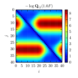
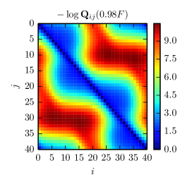
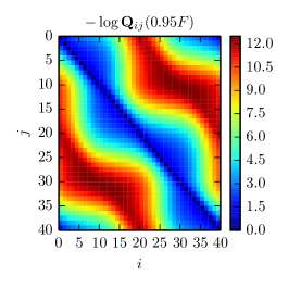
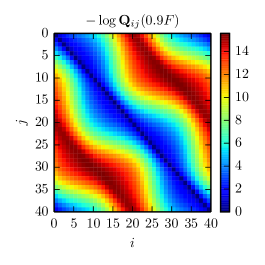
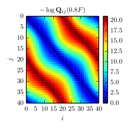
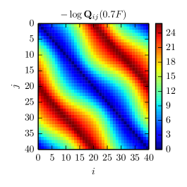
In Figure 1, we plot $-\log\mathrm{\mathbf{Q}}_{ij}(\alpha F)$ versus $i$ and $j$ for $F$ the hilly landscape transition matrix with $L=40$ and $\alpha\in\{0.7,0.8,0.9,0.95,0.98,1\}$. The purpose of this section is to give an intuitive explanation of the main features observed in the figure. Recall that the potential $V$ is shaped roughly like a “W” with peaks at $0$, $\frac{1}{2}$, and $1$ and valleys at $\frac{1}{4}$ and $\frac{3}{4}$. When $L=40$, the peaks correspond to the indices $0$, $20$, and $40$ in $\Omega$, and the valleys correspond to $10$ and $30$. (To be precise, $0$ and $40$ are identical since we take periodic boundary conditions.)

Now consider the case $\alpha=1$. We observe that $-\log\mathrm{\mathbf{Q}}_{20,j}(F)$ is small for all $j$, so $\mathrm{\mathbf{Q}}_{20,j}(F)^{-1}$ is small, and $\pi(F)$ is insensitive to perturbations which change the transition probabilities from the peak to other points. This is as expected, since the probability $\mathrm{\mathbf{P}}_{20}[\tau_{j}<\tau_{20}](F)=\mathrm{\mathbf{Q}}_{20,j}(F)$ of hitting a point $j$ in the valley before returning to the peak should be fairly large. On the other hand, $-\log\mathrm{\mathbf{Q}}_{30,10}(F)$ is enormous, so $\pi(F)$ is sensitive to the transition probability from the valley to the peak. This is also as expected, since the probability $\mathrm{\mathbf{P}}_{30}[\tau_{10}<\tau_{30}](F)$ of climbing from the valley to the peak without falling back into the valley should be small. To explain the small values of $-\log\mathrm{\mathbf{Q}}_{ij}(F)$ observed near the diagonal, we observe that for all $i\in\Omega$ and all $L$,

$$F_{i,i+1}=\frac{1}{2}\frac{1}{1+\exp\left[L\left(V\left(\frac{i+1}{L}\right)-V\left(\frac{i}{L}\right)\right)\right]}\geq\frac{1}{2}\frac{1}{1+\exp({\rm Lip}(V))}=\frac{1}{2}\frac{1}{1+\exp(1)},$$

where ${\rm Lip}(V)=1$ is the Lipschitz constant of the potential $V$. Therefore, by Corollary 1,

$$\mathrm{\mathbf{Q}}_{i,i+1}(F)^{-1}\leq\frac{1}{F_{i,i+1}}\leq 2(1+\exp(1)).$$

The same estimate holds for $\mathrm{\mathbf{Q}}_{i,i-1}(F)$.

The coefficients $\mathrm{\mathbf{Q}}_{ij}(\alpha F)$ for $\alpha<1$ share many features with $\mathrm{\mathbf{Q}}_{ij}(F)$. These coefficients would be relevant if $F$ were known with relative error $1-\alpha$; see Remark 7. The main difference between $\mathrm{\mathbf{Q}}_{ij}(\alpha F)$ and $\mathrm{\mathbf{Q}}_{ij}(F)$ is that $\mathrm{\mathbf{Q}}_{ij}(\alpha F)$ is small whenever the minimum number of time steps required to transition between $i$ and $j$ is large. The reader is directed to Section 6.5 for discussion of a related phenomenon. Observe that this effect grows more dominant as $\alpha$ decreases. We also note that $\mathrm{\mathbf{Q}}_{ij}(\alpha F)^{-1}$ is again small near the diagonal. In fact, by Lemma 3, we have

$$\mathrm{\mathbf{Q}}_{i,i+1}(\alpha F)^{-1}\leq\frac{1}{\alpha F_{i,i+1}}\leq\frac{2(1+\exp(1))}{\alpha}.$$

The same estimate holds for $\mathrm{\mathbf{Q}}_{i,i-1}(\alpha F)$.

Figure 1. Sensitivities for the hilly landscape transition matrix.

6.3. Mean first passage times and related relative error bounds

Section 4 of [2] also suggests bounds on relative error in terms of certain first passage times. A comparison is therefore in order. We record a simplified version of these results below.

Theorem 6.

[2, Corollaries 4.1,4.2] Let $F$ and $\tilde{F}$ be irreducible stochastic matrices. We have

$$\frac{\pi_{m}(\tilde{F})-\pi_{m}(F)}{\pi_{m}(F)}=\sum_{\begin{subarray}{c}i,j\in\Omega\\ i\neq j\end{subarray}}\pi_{i}(\tilde{F})((1-\delta_{jm})\mathrm{\mathbf{E}}_{j}[\tau_{m}]-(1-\delta_{im})\mathrm{\mathbf{E}}_{i}[\tau_{m}])\left(\tilde{F}_{ij}-F_{ij}\right),$$

where the expectations are taken for the chain with transition matrix $F$ and $\delta$ is the Kronecker delta function. Therefore,

$$\left\lvert\frac{\pi_{m}(\tilde{F})-\pi_{m}(F)}{\pi_{m}(F)}\right\rvert\leq\sum_{\begin{subarray}{c}i,j\in\Omega\\ i\neq j\end{subarray}}\lvert(1-\delta_{jm})\mathrm{\mathbf{E}}_{j}[\tau_{m}]-(1-\delta_{im})\mathrm{\mathbf{E}}_{i}[\tau_{m}]\rvert\left\lvert\tilde{F}_{ij}-F_{ij}\right\rvert.$$

Taking the maximum over all $m$ in the second sentence of Theorem 6 yields a pertubation result having a form similar to Theorem 3, but with

$$\beta_{ij}(F):=\max_{m\in\Omega}\lvert(1-\delta_{jm})\mathrm{\mathbf{E}}_{j}[\tau_{m}]-(1-\delta_{im})\mathrm{\mathbf{E}}_{i}[\tau_{m}]\rvert$$

in place of $\mathrm{\mathbf{Q}}_{ij}(S)^{-1}$. In the next paragraph, we show for the hilly landscape transition matrix that for some values of $i$ and $j$, $\beta_{ij}$ grows exponentially with $L$ while $\mathrm{\mathbf{Q}}_{ij}(S)^{-1}$ remains bounded. Thus, the results of [2] dramatically overestimate the error due to some perturbations.

To derive the estimate in the second sentence of Theorem 6 from the exact formula in the first sentence, one discards a factor of $\pi_{i}(\tilde{F})$. Therefore, roughly speaking, the estimate is poor when $\pi_{i}(\tilde{F})$ is small. To give a specific example, let $F$ be the hilly landscape transition matrix, assume that $L$ is even, and let $i=L/2$ and $j=L/2+1$. Observe that we have chosen $i$ at a peak of the potential $V$, so

$$\pi_{i}(F)\gtrsim\exp(-L)$$

(Here, we use the symbols $\lesssim$ and $\gtrsim$ to denote bounds up to multiplicative constants, so in the last line above, we mean that there is some $C>0$ so that the left hand side is bounded above by $C\exp(-L)$ for all $L$.) Let $F^{\varepsilon}=F+\varepsilon(e_{i}e_{j}^{\mathrm{t}}-e_{i}e_{i}^{\mathrm{t}})$. We have

$$\frac{\partial\log\pi_{m}}{\partial F_{ij}}(F)=\left.\frac{d}{d\varepsilon}\right|_{\varepsilon=0}\pi_{m}(F^{\varepsilon})=\pi_{i}(F)((1-\delta_{jm})\mathrm{\mathbf{E}}_{j}[\tau_{m}]-(1-\delta_{im})\mathrm{\mathbf{E}}_{i}[\tau_{m}])$$

by Theorem 6. Therefore, by Theorem 2,

$$\max_{m\in\Omega}\left\lvert\frac{\partial\log\pi_{m}}{\partial F_{ij}}(F)\right\rvert =\pi_{i}(F)\max_{m\in\Omega}\lvert(1-\delta_{jm})\mathrm{\mathbf{E}}_{j}[\tau_{m}]-(1-\delta_{im})\mathrm{\mathbf{E}}_{i}[\tau_{m}]\rvert$$

$$\geq\frac{1}{2}\frac{1}{\mathrm{\mathbf{P}}_{i}[\tau_{j}<\tau_{i}]},$$

and so

$$\beta_{ij}(F)\geq\frac{1}{2}\frac{1}{\pi_{i}(F)\mathrm{\mathbf{P}}_{i}[\tau_{j}<\tau_{i}]}\gtrsim\exp(L).$$

Now suppose that the substochastic matrix $S$ appearing in our bound is chosen for each $L$ so that $S_{ij}$ for $i=L/2$ and $j=L/2+1$ is bounded above zero uniformly as $L\rightarrow\infty$. For example, one might choose $S$ to be a multiple of $F$ as in Section 6.2 or a multiple of a simple random walk transition matrix as in Section 6.5. Then by Lemma 3, we have

$$\mathrm{\mathbf{Q}}_{ij}(S)^{-1}\leq\frac{1}{S_{ij}},$$

so $\mathrm{\mathbf{Q}}_{ij}(S)^{-1}$ is bounded. Thus, $\beta_{ij}(F)$ is a poor estimate of the sensitivity of the $ij^{\rm{th}}$ entry for this problem.

6.4. The spectral gap and related absolute error bounds

The survey article [3] lists eight condition numbers $\kappa_{i}(F)$ for $i=1,2,\dots,8$ for which bounds of the form

$$\left\lVert\pi(F)-\pi(\tilde{F})\right\rVert_{p}\leq\kappa_{i}(F)\left\|F-\tilde{F}\right\|_{p^{\prime}}$$

hold. (The Hölder exponents $p$ and $p^{\prime}$ vary with the choice of condition number.) Some of these condition numbers are based on ergodicity coefficients [20, 21], some on mean first passage times [2], and some on generalized inverses of the characteristic matrix $I-F$ [16, 19, 5, 9, 7]. We prove for the hilly landscape transition matrix $F$ that $\kappa_{i}(F)$ increases exponentially with $L$ for all $i$. By contrast, we have already seen that many of the coefficients $\mathrm{\mathbf{Q}}_{ij}(\alpha F)^{-1}$ are bounded as $L$ tends to infinity.

Our proof that the condition numbers increase exponentially is based on an analysis of the spectral gap of $F$. Let $\sigma(F)$ denote the spectrum of $F$. The spectral gap $\gamma$ is defined to be

$$\gamma:=1-\max\{\lvert\lambda\rvert:\lambda\in\sigma(F)\setminus\{1\}\}.$$ (29)

We use the bottleneck inequality [14, Theorem 7.3] to show that the spectral gap of the hilly landscape transition matrix decreases exponentially with $L$. For convenience, assume that $L$ is even, and let

$$E:=\left\{1,\dots,\frac{L}{2}\right\}.$$

The bottleneck ratio [14, Section 7.2] for the partition $\{E,E^{\text{\tiny c}}\}$ is

$$\Phi(E,E^{\text{\tiny c}}) =\frac{\pi\left(\frac{L}{2}\right)F_{\frac{L}{2},\frac{L}{2}+1}+\pi(1)F_{1,0}}{\frac{1}{2}}$$

$$\lesssim\frac{\exp(-L)}{1+\exp\left[L\left(V\left(\frac{1}{L}\right)-V\left(0\right)\right)\right]}$$

$$\lesssim\exp(-L).$$

(As in the last section, we use the symbols $\lesssim$ and $\gtrsim$ to denote bounds up to multiplicative constants.) Therefore, by the bottleneck inequality, the mixing time $t_{\mathrm{mix}}$ [14, Section 4.5] satisfies

$$t_{\mathrm{mix}}\geq\frac{1}{4\Phi(E,E^{\text{\tiny c}})}\gtrsim\exp(L).$$

By [14, Theorem 12.3],

$$\frac{1}{\gamma}\log\left(\frac{4}{\min\{\pi(i):i\in\Omega\}}\right)=\frac{\log(4)+L}{\gamma}\geq t_{\mathrm{mix}}.$$

Therefore,

$$\frac{1}{\gamma}\gtrsim\frac{\exp(L)}{L},$$ (30)

and we see that the spectral gap decreases exponentially in $L$.

We now relate the condition numbers to the spectral gap. Using Equation (3.3) and the table at the bottom of page 147 in [3], and also [11, Corollary 2.6], we have

$$\kappa_{i}\gtrsim\frac{1}{L\min\{|1-\lambda|:\lambda\in\sigma(F)\setminus\{1\}\}}$$ (31)

for all $i=1,\dots,8$. Now we claim that for sufficiently large $L$,

$$\gamma=1-\max\{\lvert\lambda\rvert:\lambda\in\sigma(F)\setminus\{1\}\}=\min\{|1-\lambda|:\lambda\in\sigma(F)\setminus\{1\}\},$$ (32)

in which case (30) and (31) imply that all condition numbers grow exponentially with $L$. To see this, we first observe that since $F$ is reversible, its spectrum is real [14, Lemma 12.2]. Moreover,

$$F_{ii}\geq\frac{1}{1+\exp({\rm Lip}(V))}=\frac{1}{1+\exp(1)}>0\mbox{ for all }i\in\Omega,$$

where ${\rm Lip}(V)=1$ is the Lipschitz constant of $V$. Therefore, using the Gershgorin circle theorem we have

$$\lambda\geq\frac{2}{1+\exp(1)}-1$$ (33)

for all $\lambda\in\sigma(F)$. Inequality (33) shows that $\sigma(F)$ is bounded above $-1$ uniformly in $L$, and by (30),

$$\lim_{L\rightarrow\infty}\gamma=\lim_{L\rightarrow\infty}1-\max\{\lvert\lambda\rvert:\lambda\in\sigma(F)\setminus\{1\}\}=0.$$

It follows that for sufficiently large $L$, $\max\{\lvert\lambda\rvert:\lambda\in\sigma(F)\setminus\{1\}\}$ is attained for $\lambda>0$. Thus, equation (32) holds, and we conclude using (30) and (31) that

$$\kappa_{i}\gtrsim\frac{\exp(L)}{L^{2}}$$

for all $i=1,\dots,8$.

6.5. Bounds below by a random walk

Let $Y$ be the random walk on $\Omega$ with transition matrix

$$P_{ii}=P_{i,i+1}=P_{i,i-1} :=\frac{1}{3} \mbox{ for all }i\in\Omega,\mbox{ and }$$

$$P_{ij} :=0$$ otherwise.

(As above, since $\Omega$ has periodic boundaries, $P_{L,L+1}$ means $P_{L,1}$, etc.) In this section, we use Theorem 3 to relate $\mathrm{\mathbf{Q}}_{ij}(P)$ with $\mathrm{\mathbf{Q}}_{ij}(F)$ for $F$ the hilly landscape transition matrix. First, using the lower bounds on entries of $F$ derived in Section 6.2, we have

$$F\geq\frac{3}{2}\frac{1}{1+\exp(1)}P.$$

Therefore, by (35) and Lemma 3,

$$\mathrm{\mathbf{Q}}_{ij}(\alpha F)\geq\mathrm{\mathbf{Q}}_{ij}\left(\frac{3\alpha}{2(1+\exp(1))}P\right).$$ (34)

Now for any $\beta\in(0,1)$,

$$\mathrm{\mathbf{Q}}_{ij}(\beta P) =\mathrm{\mathbf{P}}_{i}[\tau_{j}<\min\{\tau_{i},\tau_{\omega}\}](\beta P^{\omega})$$

$$=\sum_{M=1}^{\infty}\mathrm{\mathbf{P}}_{i}[\tau_{j}=M,\min\{\tau_{i},\tau_{\omega}\}>M](\beta P^{\omega}).$$

Let $\lvert i-j\rvert$ denote the minimum number of time steps required for the chain to reach state $j$ from state $i$. Adopting the notation used in the proof of Lemma 3, there is some path $\gamma\in\mathscr{P}_{ij}^{\lvert i-j\rvert}$ of length $\lvert i-j\rvert$ for which

$$\mathrm{\mathbf{Q}}_{ij}(\beta P) \geq\mathrm{\mathbf{P}}_{i}[\tau_{j}=\lvert i-j\rvert,\min\{\tau_{i},\tau_{\omega}\}>\lvert i-j\rvert](\beta P^{\omega})$$

$$\geq\mathrm{\mathbf{P}}_{i}[X_{k}=\gamma(k)\text{ for }k=1,\dots,\lvert i-j\rvert](\beta P^{\omega})$$

$$=\left(\frac{\beta}{3}\right)^{\lvert i-j\rvert}.$$ (35)

Combining (34) and (35) then yields

$$\mathrm{\mathbf{Q}}_{ij}(\alpha F)\geq\mathrm{\mathbf{Q}}_{ij}\left(\frac{3\alpha}{2(1+\exp(1))}P\right)\geq\left(\frac{3\alpha}{2(1+\exp(1))}\right)^{\lvert i-j\rvert}.$$

7. Acknowledgements

This work was funded by the NIH under grant 5 R01 GM109455-02. We would like to thank Aaron Dinner, Jian Ding, Lek-Heng Lim, and Jonathan Mattingly for many very helpful discussions and suggestions.

Appendix A Proof of Lemma 1

Proof.

Let $F$ be irreducible and stochastic. By [6, Equation (3.1)], ${\det(I-F_{i})>0}$ for all $i\in\Omega$, and

$$\pi(F)^{\mathrm{t}}=\frac{1}{\sum_{i=1}^{L}\det(I-F_{i})}(\det(I-F_{1}),\det(I-F_{2}),\dots,\det(I-F_{L})).$$ (36)

The right hand side of (36) yields the desired extension. To show this, we first observe that there exists an open neighborhood $\mathcal{V}_{F}\subset\mathbb{R}^{L\times L}$ of $F$ and a disc $\mathcal{D}_{F}\subset\mathbb{C}$ with $1\in\mathcal{D}_{F}$ such that $G\in\mathcal{V}_{F}$ implies (a) $\sum_{i}\det(I-G_{i})>0$ and (b) $G$ has exactly one eigenvalue in $\mathcal{D}_{F}$ and that eigenvalue is simple. There exists a neighborhood with property $(a)$, since $\sum_{i}\det(I-G_{i})$ is continuous in $G$ and $\sum_{i}\det(I-F_{i})>0$. The existence of a neighborhood $\mathcal{V}_{F}$ and disc $\mathcal{D}_{F}$ with property (b) follows from standard results in perturbation theory, since $F$ irreducible and stochastic implies that 1 is a simple eigenvalue of $F$; see [10, Ch. II, Theorem 5.14]. We now let $\mathcal{U}$ be the union of the sets $\mathcal{V}_{F}$ over all irreducible, stochastic $F$, and we define $\bar{\pi}:\mathcal{U}\rightarrow\mathbb{R}^{L}$ by extending the formula on the right hand side of (36). By (a), $\bar{\pi}$ is continuously differentiable. By property (b), we know that if $G\in\mathcal{U}$ with $Ge=e$ then $e$ is a simple eigenvalue of $G$, and so $\ker(I-G)=\mathbb{R}e$. Following the proof of [6, Theorem 3.1], one may then use the identity

$$(\operatorname*{adj}(I-G))(I-G)=(I-G)(\operatorname*{adj}(I-G))=0,$$

where $\operatorname*{adj}(\cdot)$ denotes the adjugate matrix, to show that $\bar{\pi}(G)^{t}G=\bar{\pi}(G)^{\mathrm{t}}$. ∎

References

- [1] A. Berman and R. J. Plemmons. Nonnegative matrices in the mathematical sciences. Academic Press (Harcourt Brace Jovanovich Publishers), New York, 1979. Computer Science and Applied Mathematics.
- [2] G. E. Cho and C. D. Meyer. Markov chain sensitivity measured by mean first passage times. Linear Algebra Appl., 316(1-3):21–28, 2000. Conference Celebrating the 60th Birthday of Robert J. Plemmons (Winston-Salem, NC, 1999).
- [3] G. E. Cho and C. D. Meyer. Comparison of perturbation bounds for the stationary distribution of a Markov chain. Linear Algebra Appl., 335:137–150, 2001.
- [4] E. Deutsch and M. Neumann. On the first and second order derivatives of the perron vector. Linear Algebra and its Applications, 71(0):57 – 76, 1985.
- [5] R. E. Funderlic and C. D. Meyer, Jr. Sensitivity of the stationary distribution vector for an ergodic Markov chain. Linear Algebra Appl., 76:1–17, 1986.
- [6] G. H. Golub and C. D. Meyer, Jr. Using the factorization and group inversion to compute, differentiate, and estimate the sensitivity of stationary probabilities for Markov chains. SIAM J. Algebraic Discrete Methods, 7(2):273–281, 1986.
- [7] M. Haviv and L. Van der Heyden. Perturbation bounds for the stationary probabilities of a finite Markov chain. Adv. in Appl. Probab., 16(4):804–818, 1984.
- [8] J. J. Hunter. Stationary distributions and mean first passage times of perturbed markov chains. Linear Algebra and its Applications, 410(0):217 – 243, 2005. Tenth Special Issue (Part 2) on Linear Algebra and Statistics.
- [9] I. C. F. Ipsen and C. D. Meyer. Uniform stability of Markov chains. SIAM J. Matrix Anal. Appl., 15(4):1061–1074, 1994.
- [10] T. Kato. Perturbation theory for linear operators. Classics in Mathematics. Springer-Verlag, Berlin, 1995. Reprint of the 1980 edition.
- [11] S. Kirkland. On a question concerning condition numbers for markov chains. SIAM Journal on Matrix Analysis and Applications, 23(4):1109–1119, 2002.
- [12] S. Kirkland and M. Neumann. Group inverses of M-matrices and their applications. Chapman & Hall/CRC applied mathematics and nonlinear science series. CRC Press, Boca Raton, 2013.
- [13] S. J. Kirkland, M. Neumann, and B. L. Shader. Applications of Paz’s inequality to perturbation bounds for Markov chains. Linear Algebra Appl., 268:183–196, 1998.
- [14] D. A. Levin, Y. Peres, and E. L. Wilmer. Markov chains and mixing times. American Mathematical Society, Providence, RI, 2009. With a chapter by James G. Propp and David B. Wilson.
- [15] C. Meyer, Jr. The role of the group generalized inverse in the theory of finite markov chains. SIAM Review, 17(3):443–464, 1975.
- [16] C. D. Meyer, Jr. The condition of a finite Markov chain and perturbation bounds for the limiting probabilities. SIAM J. Algebraic Discrete Methods, 1(3):273–283, 1980.
- [17] J. R. Norris. Markov chains, volume 2 of Cambridge Series in Statistical and Probabilistic Mathematics. Cambridge University Press, Cambridge, 1998.
- [18] C. A. O’Cinneide. Entrywise perturbation theory and error analysis for Markov chains. Numer. Math., 65(1):109–120, 1993.
- [19] P. J. Schweitzer. Perturbation theory and finite Markov chains. J. Appl. Probability, 5:401–413, 1968.
- [20] E. Seneta. Perturbation of the stationary distribution measured by ergodicity coefficients. Adv. in Appl. Probab., 20(1):228–230, 1988.
- [21] E. Seneta. Sensitivity analysis, ergodicity coefficients, and rank-one updates for finite Markov chains. In Numerical solution of Markov chains, volume 8 of Probab. Pure Appl., pages 121–129. Dekker, New York, 1991.