RESONANT ENHANCEMENT
OF MOLECULAR EXCITATION INTENSITY
IN INELASTIC ELECTRON SCATTERING
SPECTRUM OWING TO INTERACTION
WITH PLASMONS IN METALLIC NANOSHELL

Abstract

A quantum-mechanical model to calculate the electron energy-loss spectra (EELS) for the system of a closely located metallic nanoshell and a molecule has been developed.  At the resonance between the molecular excitation and plasmon modes in the nanoshell, which can be provided by a proper choice of the ratio of the inner and outer nanoshell radii, the cross-section of inelastic electron scattering at the molecular excitation energy is shown to grow significantly, because the molecular transition borrows the oscillator strength from a plasmon.  The enhancement of the inelastic electron scattering by the molecule makes it possible to observe molecular transitions with an electron microscope.  The dependences of the EEL spectra on the relative arrangement of the molecule and the nanoshell, the ratio between the inner and outer nanoshell radii, and the scattering angle are plotted and analyzed.

1 Introduction

In the last years, a relatively new domain of researches, plasmonics, develops intensively [1].  It uses the ability of collective electron oscillations in metals to enormously strengthen electric fields [2] for studying various physical systems and developing new methods of researches in science [3], engineering [4], and medicine [5].

The plasmon resonance is studied using the methods based on the interaction of plasmons with light, electrons, or atoms.  One of those methods is the electron energy-loss spectroscopy (EELS).  The high resolution of an electron microscope (down to 1 Å) allows the effect of plasmon resonance on nano-dimensional objects to be observed with a better spatial resolution than other spectroscopic methods permit.  In the recent years, the EELS was used to study nanoparticles of various shapes [6], the interaction between nanoparticles [7], thin films [8], and composite nano-materials [9].  The authors of work [10] studied plasmon excitations in silver nanorods and showed that the plasmon excitations are quantized into resonance modes, with the intensity of mode maxima changing along the nanorod, and the plasmon wavelength being minimum at the nanorod ends.  In work [11] on the basis of electron tomography, the method of localized plasmon mode imaging was developed using a three-dimensional nano-sized cube as an example, and a capability to single-out every mode from the total output signal with regard for the substrate and the shape of a nano-dimensional object was demonstrated.

This work aims at studying the possibility to observe the excitation of an organic molecule in EEL spectra owing to the resonant interaction between the molecule and localized plasmons in a nanoparticle or a nanoshell.  The oscillator strength of the molecule in the excited state can considerably grow at its resonant mixing with plasmon excitations in the nanoparticle due to a large dipole moment of localized plasmons.  This enhancement is especially pronounced in the surface enhancement of Raman spectra [12] and, to some less extent, in fluorescence spectra [13].  A similar effect should expectedly take place for the EEL spectra as well, which would enable separate molecules adsorbed on the nanoparticle surface to be observed with an electron microscope.

For the theoretical calculation of EEL spectra, a quantum-mechanical approach developed in works [14,​ 15] is applied.  This procedure includes the calculation of the classical plasmon spectrum for a metallic nanoparticle, the quantization of normal modes, the calculation of the spectrum of the composite system taking the plasmon interaction and the molecule excitation into account, and the calculation of the cross-sections of inelastic electron scattering with the excitation of the obtained states.

The mixing of localized plasmon states with molecular ones has a resonant character.  At the same time, the properties of localized plasmons depend on nanoparticle’s shape [16,​ 17] and size [18].  This circumstance makes it possible to reach the effective interaction between plasmons and the molecule by choosing the corresponding shape of a nanoparticle.  The inelastic electron scattering at a spherical nanoparticle was considered in work [19].  In the present work, we analyze the more complicated case of a spherical nanoshell.

2 Model of the System

The system consisting of a molecule near a spherical metallic nanoshell is considered (Fig.  1).  The spectrum of molecular excitations is simulated as a two-level system with the transition moment $\mathbf{d}$.  The distance between the molecule and the nanoparticle surface equals $L$.  The outer radius of the nanoshell is $R_{2}$, the inner one is $R_{1}$.  The nanoshell radius $R_{2}$ is supposed to be small in comparison with the length of electromagnetic waves, whose frequency corresponds to the plasmon frequency, $R_{2}\ll c/\omega_{p}$, where $c$ is the speed of light, and $\omega_{p}$ is the plasma frequency.  The molecule can be oriented arbitrarily with respect to the nanoparticle and the high-energy electron beam propagation direction.  We suppose that an electron beam with wavevector $\mathbf{k}$ falls on the system concerned and is scattered into a state with the wavevector $\mathbf{k}^{\prime}$.

The spectrum of nanoshell plasmon oscillations has two modes, which correspond roughly to oscillations on the outer and inner surfaces. Therefore, the first problem consists in finding the frequencies of those modes and their dependences on the ratio between the inner and outer radii. Below, it will be demonstrated that, by choosing this ratio, it is possible to reach a resonance between the excitation energies of the molecule and a localized plasmon.

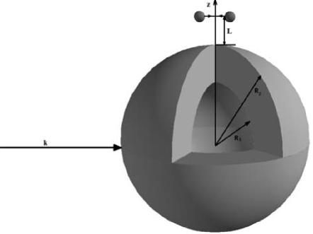
Fig. 1.: Scheme of the electron scattering by the system consisting of a spherical nanoshell with inner radius $R_{1}$ and outer radius $R_{2}$, and the molecule-dipole at a distance $L$

The next step in the calculation procedure is the quantization of plasmon oscillations and the determination of the mixed-mode spectrum taking into account the interaction between the molecule modeled as a two-level system and localized plasmons.  The probability of the electron scattering with the excitation of those mixed modes is calculated in the Born approximation.

3 Surface Plasmons
on a Spherical Metallic Nanoshell

The nanoshell is considered in the quasistatic approximation, i.e.  the nanoparticle radius is supposed to be much smaller than the wavelength, $R\ll c/\omega$.  This approximation allows us to characterize the electromagnetic field by the electrostatic potential $\phi$.

To find the spectrum of localized plasmons in the nanoshell, we have to consider the electromagnetic field in three regions: the dielectric core, metallic shell, and external region.  The field in the metallic shell interacts with free electrons.  We will consider the electron subsystem of the metal, by using the Drude model.

The polarization $\mathbf{P}$ of the electron subsystem in the electrostatic potential – as a consequence of Newton’s equation of motion for free electrons, $m\ddot{\mathbf{r}}=-e\mathbf{E}=$ $=e\nabla\phi$ – is described by the equation

$$\ddot{\mathbf{P}}=-en\ddot{\mathbf{r}}=-\frac{ne^{2}}{m}\nabla\phi,$$ (1)

where $m$ is the electron mass, $e$ the electron charge, and $n$ the electron concentration. This equation has to be solved together with Maxwell’s equation for the electric field,

$$\nabla\cdot\mathbf{D}=\varepsilon_{0}\nabla^{2}\phi+4\pi\nabla\cdot\mathbf{P}=0,$$ (2)

where $\varepsilon_{0}$ is the contribution of all factors, except for free electrons, to the dielectric permittivity.

It is convenient to seek the polarization in the form $4\pi\mathbf{P}=-\nabla\psi$, where $\nabla^{2}\psi=0$.  Then the field equation (2) reads

$$\nabla^{2}\phi=0,$$ (3)

and Eq. (1) transforms into

$$\ddot{\psi}=\omega_{p}^{2}\phi,$$ (4)

where $\omega_{p}=\sqrt{\frac{4\pi e^{2}n}{m}}$ is the plasma frequency.  Equations (3) and (4) have to be solved together with the continuity conditions for the potential $\phi$ and the normal component of the electric induction vector,

$$\mathbf{D_{n}}=-\varepsilon_{0}\nabla\phi-\nabla\psi.$$ (5)

The fields in three regions – the dielectric core of the nanoshell, the metallic layer, and the environment – are sought in the following general forms:

$$\phi^{(1)}=\sum_{lm}a_{lm}^{(1)}r^{l}Y_{lm}(\theta,\varphi),$$ (6)

$$\left\{\begin{aligned} \!\!\phi^{(2)}=\sum_{lm}(a_{lm}^{(2)}r^{l}+b_{lm}^{(2)}r^{-l-1})Y_{lm}(\theta,\phi),\\ \!\!\psi^{(2)}=\sum_{lm}(c_{lm}^{(2)}r^{l}+d_{lm}^{(2)}r^{-l-1})Y_{lm}(\theta,\phi),\\ \end{aligned}\right.$$ (7)

$$\phi^{(3)}=\sum_{lm}a_{l}^{(3)}r^{-l-1}Y_{lm}(\theta,\varphi).$$ (8)

Applying the continuity conditions for the potential and the normal component of the electric induction vector, we obtain a system of equations for the coefficients $a_{lm}$, $b_{lm}$, $c_{lm}$, and $d_{lm}$:

$$\left\{\begin{array}[]{l}a_{lm}^{(1)}=a_{lm}^{(2)}+b_{lm}^{(2)}R_{1}^{-2l-1},\\[5.69054pt] a_{lm}^{(2)}+b_{lm}^{(2)}R_{2}^{-2l-1}=b_{lm}^{(3)}R_{2}^{-2l-1},\\[5.69054pt] -\varepsilon^{(1)}la_{lm}^{(1)}=\mathbf{D_{n}}^{(2)},\\[5.69054pt] -\varepsilon^{(3)}\frac{l+1}{R_{2}^{2l+1}}b_{lm}^{(3)}=\mathbf{D_{n}}^{(2)},\\ \end{array}\right.$$ (9)

where $D_{\mathbf{n}}^{(2)}=\varepsilon_{0}\frac{l+1}{R_{1}^{2l+1}}b_{lm}^{(2)}-\varepsilon_{0}la_{lm}^{(2)}+\frac{l+1}{R_{1}^{2l+1}}d_{lm}^{(2)}-lc_{lm}^{(2)}$ is the normal component of the electric induction vector in the metallic layer.

The solution of this system makes it possible to relate all unknown variables to the coefficients $c_{lm}^{(2)}$ and $d_{lm}^{(2)}$ that express the electromagnetic field in the metallic layer.  Substituting those solutions into Eq. (4), we obtain a system of equations for the plasmon modes,

$$\left\{\!\begin{aligned} \ddot{c}_{lm}^{(2)}-\omega_{p}^{2}A_{lm}^{11}{c}_{lm}^{(2)}-\omega_{p}^{2}A_{lm}^{12}{d}_{lm}^{(2)}=0,\\ \ddot{d}_{lm}^{(2)}-\omega_{p}^{2}A_{lm}^{21}{c}_{lm}^{(2)}-\omega_{p}^{2}A_{lm}^{22}{d}_{lm}^{(2)}=0.\end{aligned}\right.$$ (10)

The coefficients $A_{lm}$ are given in Appendix.

System (10) is a system of equations for coupled oscillators.  The corresponding equations for two normal modes for every $l$ and $m$ look like

$$\ddot{q}_{lm}^{\pm}+\left(\omega_{l}^{\pm}\right)^{2}q_{lm}^{\pm}=0.$$ (11)

The normal mode frequencies are determined by the formula

$$(\omega_{l}^{(\pm)}/\omega_{p})^{2}=-\frac{A_{lm}^{11}+A_{lm}^{22}}{2}\,\pm$$

$$\pm\,\sqrt{\frac{(A_{lm}^{11}-A_{lm}^{22})^{2}}{4}+A_{lm}^{21}A_{lm}^{12}}.$$ (12)

Accordingly, the coefficients $c_{lm}^{(2)}$ and $d_{lm}^{(2)}$ in Eqs. (10) are expressed in terms of the coefficients $q_{lm}^{\pm}$ as follows:

$$c_{lm}^{(2)}=q_{lm}^{+}+q_{lm}^{-},$$ (13)

$$d_{lm}^{(2)}=-\frac{(\omega_{l}^{+})^{2}+\omega_{p}^{2}A^{11}_{lm}}{\omega_{p}^{2}A^{12}_{lm}}q_{lm}^{+}\,-$$

$$-\,\frac{(\omega_{l}^{-})^{2}+\omega_{p}^{2}A_{lm}^{11}}{\omega_{p}^{2}A_{lm}^{12}}q_{lm}^{-}.$$ (14)

In Fig. 2, the oscillation frequencies versus the ratio between the outer and inner nanoshell radii are shown for two dipole modes ($l=1$).  If the metallic layer thickness is large, those modes can be regarded as plasmons localized on the inner and outer surfaces of the shell, and their frequencies are equal to the frequencies of localized plasmons in a solid particle and the pore in a metal, respectively.  As the metallic layer becomes thinner, the interaction between oscillations on two surfaces gets stronger, which gives rise to considerable variations in the spectrum.  This is especially actual for the lower mode, which corresponds to the outer surface.  For a silver nanoshell, the choice of the ratio between the radii allows one to reduce the plasmon frequency from the ultra-violet spectral range to the visible and even infra-red one if the metallic layer is very thin.  Hence, we obtain a possibility to select nanoshells, the plasmon oscillations in which will be in resonance with the molecular transition frequency.

3.1 Quantization of the nanoshell field

While determining the intensity of the interaction between plasmon oscillations in the nanoshell and other particles – atoms, molecules, or high-energy electrons – we used the quantization approach for the electromagnetic field of plasmons, which was developed and applied in works [14,​ 15,​ 20,​ 21].  The quantization procedure begins with the determination of the proper action functional: by varying its variables, we can obtain the equations of motion.  In the case of a nanoshell, the action functional must be a start point for the derivation of the equation for the electromagnetic field, the equation of motion for the electron polarization in the metallic layer, and the boundary conditions at the inner and outer surfaces.  The corresponding action looks like

$$S=\int\limits_{0}^{t}(\mathcal{L}_{\rm core}+\mathcal{L}_{\rm metal}+\mathcal{L}_{\rm outer})dt,$$ (15)

where

$$\mathcal{L}_{\rm core}=\frac{1}{4\pi}\int\limits_{V_{\rm core}}\frac{\varepsilon^{(1)}}{2}(\nabla\phi)^{2}dV,$$ (16)

$$\mathcal{L}_{\rm metal}=\frac{1}{4\pi}\int\limits_{V_{m}}\Biggl{[}\frac{\varepsilon_{0}}{2}(\nabla\phi)^{2}-4\pi\mathbf{P}\nabla\,\phi\,+$$

$$+\left(\!\frac{4\pi}{\omega_{p}}\!\right)^{\!\!2}\frac{1}{2}\,\dot{\mathbf{P}}^{2}\Biggr{]}dV,$$ (17)

$$\mathcal{L}_{\rm outer}=\frac{1}{4\pi}\int\limits_{V_{\rm core}}\frac{\varepsilon^{(3)}}{2}(\nabla\phi)^{2}dV.$$ (18)

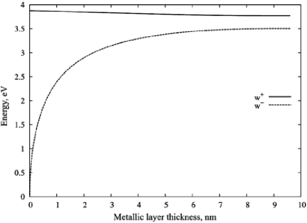
Fig. 2.: Dependences of the plasma oscillation energy on the silver nanoshell thickness.  The outer radius equals 10 nm, and the inner one changes from 0.5 to 9.5 nm

Substituting the corresponding expressions for the fields, Eqs. (6)–(8), and carrying out a cumbersome integration, we reduce the Lagrangian density to the classical oscillator form,

$$\mathcal{L}=\frac{1}{2}\sum_{lm}\biggl{\{}\!\left[\left(\dot{Q}_{lm}^{+}\right)^{\!2}-\left(\omega_{l}^{+}\right)^{2}\left(Q_{lm}^{+}\right)^{2}\right]+$$

$$+\left[\left(\dot{Q}_{lm}^{-}\right)^{\!2}-\left(\omega_{l}^{+}\right)^{2}\left(Q_{lm}^{-}\right)^{2}\right]\!\biggr{\}},$$ (19)

where the variables $Q_{lm}^{-}$ and $Q_{lm}^{+}$ are proportional to the variables $Q_{lm}^{\pm}=\sqrt{B_{lm}^{\pm}}q_{lm}^{\pm}$ introduced above (the $B_{lm}$-values are given in Appendix).

The transition to quantum-mechanical operators is carried out, by following the canonical quantization procedure of oscillator variables and equating the quantum energy to $\hbar\omega_{l}^{\pm}$.  As a result of the quantization, we can write the electric potential of plasma oscillations in terms of the plasmon creation, $\hat{Q}_{lm}^{\mu\dagger}$, and annihilation, $\hat{Q}_{lm}^{\mu}$, operators,

$$\hat{\phi^{(1)}}=\sum_{lm\mu}\sqrt{\frac{\hbar}{2\omega_{l}^{\mu}B_{l}^{\mu}}}N_{l}^{\mu}r^{l}(\hat{Q}_{lm}^{\mu\dagger}+\hat{Q}_{lm}^{\mu})Y_{lm}(\theta,\varphi),$$ (20)

$$\hat{\phi^{(2)}}=\sum_{lm\mu}\sqrt{\frac{\hbar}{2\omega_{l}^{\mu}B_{l}^{\mu}}}\left(\!F_{l}^{\mu}\frac{1}{r^{l+1}}+\left(\!\frac{\omega_{l}^{\mu}}{\omega_{p}}\!\right)^{\!\!2}r^{l}\!\right)\!\times$$

$$\times\,(\hat{Q}_{lm}^{\mu\dagger}+\hat{Q}_{lm}^{\mu})Y_{lm}(\theta,\varphi),$$ (21)

$$\hat{\phi^{(3)}}=\sum_{lm\mu}\sqrt{\frac{\hbar}{2\omega_{l}^{\mu}B_{l}^{\mu}}}K_{l}^{\mu}\,\times$$

$$\times\,\frac{1}{r^{l+1}}(\hat{Q}_{lm}^{\mu\dagger}+\hat{Q}_{lm}^{\mu})Y_{lm}(\theta,\varphi),$$ (22)

where the subscript $\mu$ acquires the values “$+$” and “$-$”, and the formulas for $N_{l}$, $F_{l}$, and $K_{l}$ are given in Appendix.  Below, when summing up over $l$, only the first term of the series will be taken into consideration, because the higher terms give an insignificant contribution to the field expression, i.e.  we are limited the dipole approximation ($l=1$).

3.2 Mixed excitation spectrum
for the molecule and the nanoshell

The interaction between electrons in the molecule and the electron subsystem in the nanoparticle results in the mixing of quantum states in both subsystems of our system.  This mixing can be substantial if it has a resonant character, i.e.  if the energy of the excited state of the molecule is close to the energy of a plasmon in the nanoparticle.  We consider the molecule as a two-level system with the dipole moment $\mathbf{d}$ (Fig. 1) and the creation and annihilation operators $\hat{c}^{\dagger}$ and $\hat{c}$, respectively.

The total Hamiltonian of the system “molecule + nanoparticle”, which involves the interaction between them in the dipole approximation, looks like

$$H=\sum\limits_{1m\mu}(\hbar\omega_{1}^{\mu}\hat{Q}_{1m}^{\mu\dagger}\hat{Q}_{1m}^{\mu})+E_{0}\hat{c}^{\dagger}\hat{c}-\mathbf{d}\nabla\phi(\mathbf{r})(\hat{c}^{\dagger}+\hat{c}).$$ (23)

The interaction between the molecule and the nanoshell is described by the last term in this Hamiltonian, in which the operator of nanoparticle electrostatic potential is taken at the point $\mathbf{r}$, where the molecule is located.  The diagonalization of Hamiltonian (23) gives us the spectrum and the wave functions of the system.

It is convenient to change from the operators $\hat{Q}_{lm}^{\mu\dagger}$ and $\hat{Q}_{lm}^{\mu}$ to the operators $Q_{p}^{\mu}$ and $Q_{p}^{\mu\dagger}$, where the subscript $p$ runs through the values $\left(x,y,z\right)$ according to the relations

$$\hat{Q}_{x}^{\mu\dagger}\!=(\hat{Q}_{1-1}^{\mu\dagger}-\hat{Q}_{11}^{\mu\dagger})/\sqrt{2},$$

$$\hat{Q}_{y}^{\mu\dagger}\!=\imath(\hat{Q}_{1-1}^{\mu\dagger}+\hat{Q}_{11}^{\mu\dagger})/\sqrt{2},$$

$$\hat{Q}_{z}^{\mu\dagger}=\hat{Q}^{\mu\dagger}_{10}.$$

The eigenvalues of the Hamiltonian – there are 7 of them – give the energy spectrum of the system. The spectrum of plasmons in the nanoshell is triple-degenerate with respect to the magnetic quantum number $m$ of the molecule.  However, the presence of the molecule results in a partial lift of this degeneration.  The obtained spectrum contains two degenerate levels of surface plasmons for each of the energies $\hbar\omega_{1}^{+}$ and $\hbar\omega_{1}^{-}$.  The third level shifts as a result of the interaction with the molecule.  The split of surface plasmon levels and a shift of the molecular excitation energy depend on the distance between the dipole and the particle and on the orientation of the dipole moment of a molecular transition.

The creation operators for the mixed states are determined in terms of characteristic vectors of the whole system and are given by the relations

$$\hat{\psi}_{j}^{\dagger}=\sum\limits_{p=1}^{3}S_{jp}\hat{Q}_{p}^{+\dagger}+\sum\limits_{p=4}^{6}S_{jp}\hat{Q}_{p}^{-\dagger}+S_{j7}\hat{c}^{\dagger},$$ (24)

where $S_{jp}$ is a unitary matrix determined while diagonalizing the Hamiltonian (in the course of further calculations, the Hamiltonian was diagonalized numerically).  Accordingly, taking into account that $S_{jp}$ is a real-valued matrix, the creation operators $\hat{Q}_{p}^{\mu\dagger}$ required for the further calculations can be expresses in terms of the new operators of mixed excitations, $\hat{\psi}_{j}^{\dagger}$, as follows:

$$\hat{Q}_{p}^{+\dagger}=\sum\limits_{j=1}^{7}S_{pj}\hat{\psi}_{j}^{\dagger},\quad\hat{Q}_{s}^{-\dagger}=\sum\limits_{j=1}^{7}S_{sj}\hat{\psi}_{j}^{\dagger},$$ (25)

where $p=\left\{1,2,3\right\}$ and $s=\left\{4,5,6\right\}$.  For the creation operator of a molecular excitation $\hat{c}^{\dagger}$, we have

$$\hat{c}^{\dagger}=\sum_{j=1}^{7}S_{7j}\hat{\psi}_{j}^{\dagger}.$$ (26)

Similar expressions can be obtained for the annihilation operators $\hat{Q}_{p}^{+}$, $\hat{Q}_{s}^{-}$, and $\hat{c}$.

4 Calculation of Electron Scattering Spectra

Let the electron, which is regarded as a quantum-mechanical particle with the initial energy $E$, be scattered by the system “molecule–nanoshell”.  The wave function of the incident electron is a plane wave with the wave vector $\mathbf{k}$.  A detector registers electrons with the wave vector $\mathbf{k}^{\prime}$.  The general scattering setup is illustrated in Fig. 3.

The general form of the Hamiltonian for an electron interacting with the examined system looks like

$$\hat{H}=-\frac{\hbar^{2}\Delta}{2m_{e}}+\hat{H}_{S}+\hat{H}_{\rm int},$$ (27)

where the first term is the operator of the electron kinetic energy, $\hat{H}_{S}$ is the Hamiltonian of the system, and $\hat{H}_{\rm int}$ the operator of interaction between the electron and the system.

The Hamiltonian of the system $\hat{H}_{S}$ can be written in the form of a series expansion in the normal oscillation modes of the system.  Then, the operator of interaction between the system and the external electron, $\hat{H}_{S}=-e\Phi(\mathbf{r})$, contains terms proportional to the creation and annihilation operators of normal modes.  The interaction intensity is calculated as the electrostatic potential of the excitation at the point, where the electron is located.

The effective electron scattering cross-section per unit solid angle can be determined from the general relation [22]

$$d\sigma=|f(\mathbf{k},\mathbf{k^{\prime}})|^{2}d\Omega,$$ (28)

where $f(\mathbf{k},\mathbf{k^{\prime}})$ is the electron scattering amplitude.  We consider electrons to be fast enough to treat the scattering field $\Phi$ as a perturbation.  Under those conditions, the formula for the scattering amplitude in the Born–Oppenheimer approximation looks like

$$f(k,k^{\prime})=-\frac{m_{e}}{2\pi\hbar^{2}}V_{\mathbf{Q}n}=-\frac{m_{e}}{2\pi\hbar^{2}}\int e^{i\mathbf{Q}\mathbf{r}}\Phi(\mathbf{r})d^{3}r,$$ (29)

where $V_{\mathbf{Q}n}$ is the matrix element for the electron transition from the state $k$ into the state $k^{\prime}$ with the excitation of the $n$-th mode in the system, and $\mathbf{Q}\,{=}\,\mathbf{k}\,{-}\,\mathbf{k^{\prime}}$ is the transferred momentum, as is shown in Fig. 3.

In order to calculate the double differential scattering cross-section defined by the expression

$$\frac{d\sigma}{d\Omega dE}=\frac{m^{2}}{4\pi^{2}\hbar^{4}}V_{\mathbf{Q}n}^{2}\delta(\Delta E-E_{l}),$$ (30)

where $\Delta E=(k^{2}-k^{\prime 2})/2m$ is the energy lost by the electron, and $E_{l}$ are the resonance energies, it is necessary to find the transition matrix element $V_{\mathbf{Q}n}$.  In the following sections, we will separately consider the cases of the electron scattering by the nanoshell, the molecule, and the system composed of the nanoshell and the molecule.

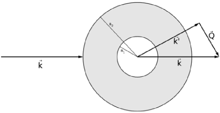
Fig. 3.: Scheme of the electron scattering by a spherical nanoshell with inner radius $R_{1}$ and outer radius $R_{2}$

4.1 Inelastic electron
scattering by the nanoshell

For the electron scattered by a conducting nanoshell, the interaction Hamiltonian looks like

$$H_{\rm int}=-e\phi(\mathbf{r}),$$ (31)

where $\phi(\mathbf{r})$ is the field determined by formulas (20), (21), and (22) for three regions: the core, metallic layer, and external space, respectively.  Only three modes are excited in the dipole approximation: with $l=1$ and $m=0,\pm 1$.  It is convenient to calculate the matrix element in a coordinate system with the applicate axis directed along the vector $\mathbf{Q}$ and choose the same coordinate frame for normal modes.  In this frame, only the mode with $m=0$ is excited.

In the spherical coordinate system, the matrix element of the electron transition reads

$$V_{Q,1,0}^{(\rm shell)}=-e\iiint\sin{\theta\,}r^{2}e^{iQr\cos{\theta}}\phi(r)drd\theta d\varphi.$$ (32)

It is convenient to use the formula

$$e^{iQr\cos{\theta}}=\sum_{l=0}^{\infty}(2l+1)i^{l}j_{l}(Qr)P_{l}(\cos{\theta}).$$ (33)

Hence, it remains only to integrate over the radial variable, with the corresponding interval being divided into three regions: the nanoshell core, metallic layer, and region outside the nanoshell.  Those integrals are reduced to the following ones to within coefficients: $I_{1}=\int_{0}^{R}\chi^{3}j_{1}(\alpha\chi)d\chi$, $I_{2}=\int_{R}^{1}\chi^{3}j_{1}(\alpha\chi)d\chi$, $I_{3}=\int_{R}^{1}j_{1}(\alpha\chi)d\chi$, and $I_{4}=\int_{1}^{\infty}j_{1}(\alpha\chi)d\chi$ with the dimensionless variables $\chi=r/R_{2}$, $\alpha=QR_{2}$, and $R=R_{1}/R_{2}$.  The matrix elements $V_{Q,1,0}^{(\rm shell)}$ can be the calculated with the help of the formula

$$V_{Q,1,0}^{(\rm shell)}=i\sqrt{\frac{27\pi\hbar e^{2}}{2\omega_{1}^{\mu}B_{1}^{\mu}}}\biggl{\{}R_{2}^{4}N_{1}^{\mu}I_{1}+R_{2}^{4}\left(\!\frac{\omega_{1}^{\mu}}{\omega_{p}}\!\right)^{\!\!2}I_{3}\,+$$

$$+\,R_{2}F_{1}^{\mu}I_{2}+R_{2}K_{1}^{\mu}I_{4}\biggr{\}}\!,$$ (34)

where, as was already mentioned above, the superscript $\mu$ acquires the values “$+$” and “$-$”.  Therefore, for the sake of convenience, we split the expression obtained for $V_{Q,1,0}^{(\rm shell)}$ into $V_{Q,1,0}^{+(\rm shell)}$ and $V_{Q,1,0}^{-(\rm shell)}$, respectively.  The integrals $I_{n}$ were calculated numerically.

4.2 Inelastic electron scattering
giving rise to the molecule excitation

For an electron scattered by the molecule, the Hamiltonian of their interaction looks like

$$H_{\rm int}=-eW(\mathbf{r})(c^{\dagger}+c)=-e\frac{\mathbf{d}\,\mathbf{r}}{r^{3}}(c^{\dagger}+c),$$ (35)

where $c^{\dagger}$ and $c$ are the creation and annihilation, respectively, operators for the molecule transition from the ground state into the excited one and backward.  Taking expression (29) for the scattering amplitude into account, the matrix elements of the system should be sought in the form

$$W_{Q}^{(\rm dip)}=-e\int W(\mathbf{r})e^{i\mathbf{Q}\,\mathbf{r}}d^{3}r.$$ (36)

As was done in the case of a nanoshell, we select the direction of the applicate axis along the vector of transferred momentum $\mathbf{Q}$.  Changing to the spherical coordinate system and making allowance for the series expansion (33) of exponential function, we can integrate over the angles $\phi$ and $\theta$.  Since $\mathbf{d}$ is directed along the vector $\mathbf{Q}$, the component $d_{z}$ can be expressed in terms of those two vectors, which are independent of the radial variable $r$. As a result of the indicated operations, we obtain the following expression for the matrix element $W_{Q}^{(\rm dip)}$:

$$W_{Q}^{(\rm dip)}=4\pi ei\frac{\mathbf{d}\,\mathbf{Q}}{Q}\int\limits_{0}^{\infty}j_{l}(Qr)dr=4\pi ei\frac{\mathbf{d}\,\mathbf{Q}}{Q^{2}}.$$ (37)

The resonant energy, which is used in expression (30) for the double differential cross-section is the energy of the dipole transition between the molecule levels, $E_{0}$.

4.3 Inelastic electron scattering
by the system consisting of the molecule
and the nanoshell

The operator of electron interaction with the system consisting of the molecule and the nanoshell can be written in the form

$$H_{\rm int}=\sum_{m}(V_{m}^{\mu}\hat{Q}_{m}^{\mu\dagger}+V_{m}^{\mu\ast}\hat{Q}_{m}^{\mu})+W\hat{c}^{\dagger}+W^{\ast}\hat{c},$$ (38)

where $V_{m}^{\mu}$ is the potential of interaction between the electron and plasmons on the nanoshell surface, and $W$ the potential of interaction between the molecule and the electron.

For the further calculation of matrix elements, let us express the perturbation in terms of the mixed state operators of the system, $\hat{\psi}_{j}^{\dagger}$ and $\hat{\psi}_{j}$, which are defined by formulas (25) and (26),

$$H_{\rm int}=\sum_{j=1}^{7}\Biggl{(}\,\sum_{p=1}^{3}V_{p}^{+}(\mathbf{r})S_{pj}\,+$$

$$+\sum_{p=3}^{6}V_{p}^{-}(\mathbf{r})S_{pj}+W(\mathbf{r})S_{7j}\!\Biggr{)}\hat{\psi}^{\dagger}_{j}+{\rm c.t.}$$ (39)

With regard for the expressions for the electron scattering at the nanoshell, Eq. (34), and the molecule, Eq. (37), we obtain the following formula for the matrix elements $V_{Qn}(\Theta_{\rm sc})$ of the electron transition at its scattering by the system consisting of the nanoshell and the molecule:

$$V_{Qn}(\Theta_{\rm sc})=S_{7j}W_{Q}^{(\rm dip)}+(S_{1j}\sin\Theta_{\rm sc}\cos\phi_{\rm sc}\,+$$

$$+\,S_{2j}\sin\Theta_{\rm sc}\sin\phi_{\rm sc}+S_{3j}\cos\Theta_{\rm sc})V_{Q,1,0}^{+(\rm shell)}\,+$$

$$+\,(S_{4j}\sin\Theta_{\rm sc}\cos\phi_{\rm sc}\,+$$

$$+\,S_{5j}\sin\Theta_{\rm sc}\sin\phi_{\rm sc}+S_{6j}\cos\Theta_{\rm sc})V_{Q,1,0}^{-(\rm shell)}$$ (40)

where $\Theta_{\rm sc}$ and $\phi_{\rm sc}$ are the electron scattering angles.  The coefficients $S_{ij}$ can be calculated by diagonalizing the Hamiltonian (Section 2.2).  The integrals $V_{Q,1,0}^{\mu(\rm shell)}$ are calculated independently and, therefore, have the same form as in Section 3.1. The difference consists is that the coefficients $S_{ij}$ include the interaction between the molecular excitation and the plasmon modes.  For example, the coefficient $S_{7j}$ can exceed 1 very much, because the molecule excitation “borrows” the oscillator strength from the plasmon. Just this difference increases the probability of the molecule excitation near metallic nanoshells.

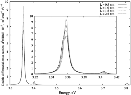
Fig. 4.: EEL spectra for various distances $L$ between the shell and the molecule.  Electrons are scattered by the system consisting of a silver shell with the outer radius $R_{2}\,{=}\,7.5$ nm and the inner radius $R_{1}\,{=}\,4$ nm , and a molecule with the dipole moment $d\,{=}\,10\leavevmode\nobreak\$D.  ${E_{k}=10\leavevmode\nobreak\ }\mathrm{keV}$, $\hbar w_{p}=11.5853$$\leavevmode\nobreak\ \mathrm{eV}$, $\varepsilon_{0}=8.926$, and $\hbar\omega_{0}\,{=}\,3.4$$\leavevmode\nobreak\ \mathrm{eV}$. The molecule has the orientation $\left({\Theta\,{=}\,\pi/6,\phi\,{=}\,\pi/6}\right)$ with respect to the shell

5 Results and Discussion

The EEL spectra were calculated for a silver nanoshell, the dielectric function of which is described by the parameters: $\hbar\omega_{p}=11.5853\leavevmode\nobreak\ \mathrm{eV}$ and $\varepsilon_{0}=8.926$. The inner nanoshell radius was selected to be 4 nm, whereas the outer radius was varied from 7.5 to 10 nm.  The dipole moment of the molecule changed in the limits from 5 to 12 D.  In the majority of calculations, the molecule was considered to be at a distance of 1 nm from the shell surface.  The energy of dipole transition in the molecule was $\hbar\omega_{0}=3.4\leavevmode\nobreak\ \mathrm{eV}$.  The energy of the fast electron was 10⁴ eV.  The transferred momentum $Q$ increases as the scattering angle grows.  Since the scattering amplitude decreases for larger transferred momenta at least as $1/Q^{2}$, the calculations were carried out for the angles $\Theta_{\rm sc}=0$ and $\phi_{\rm sc}=0$, i.e.  the forward scattering was considered.

While calculating the double differential scattering cross-section, the delta-function was replaced by the Lorentzian

$$\delta(\Delta E-E_{j})=\frac{1}{\pi}\frac{\Gamma}{(\Delta E-E_{j})^{2}+\Gamma^{2}},$$ (41)

where $\Gamma$ is a phenomenological parameter that describes the line broadening for the surface plasmon.  In our calculations, we took $\Gamma=3$$\div$$5$ meV.

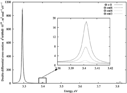
Fig. 5.: EEL spectra for various angles $\theta$ of the molecule orientation with respect to the nanoshell.  Electrons are scattered by the system consisting of a silver shell and a molecule at a distance of 1 nm.  The other parameters are the same as in Fig. 4

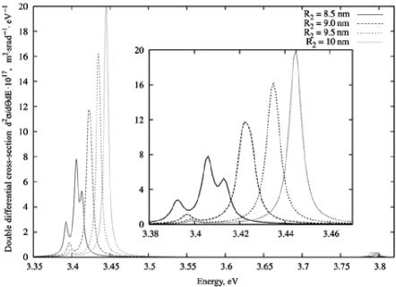
Fig. 6.: EEL spectra for various ratios $R_{2}/R_{1}$ between the outer and inner nanoshell radii.  The outer radius $R_{2}$ was varied, the inner one was fixed, $R_{1}=4$ nm. The distance between the molecule and the shell equals 1 nm.  The other parameters are the same as in Fig. 4

In Figs.  4 to 6, three peaks are observed.  The most intensive peak is located at the oscillation frequency of a plasmon on the outer shell surface.  The peak corresponding to the molecule excitation enhancement is located near to it.  The least intensive peak is located at the oscillation frequency of a plasmon on the inner shell surface (at about 3.8 eV).  The inset in each figure demonstrates the scaled-up right section of the corresponding spectrum.

The main contribution to the molecule excitation enhancement is given by the plasmon mode on the outer nanoshell surface.  The frequency of the modes on the nanoshell surfaces depends on the ratio between the inner and outer radii.  By varying this ratio, we can obtain the required resonant frequency of plasmons (Fig. 6). This is the advantage of a shell in comparison with a solid nanoparticle, on the surface of which only one mode, whose frequency is almost independent of the particle radius, emerges.  Figure 6 illustrates the “borrowing” of the oscillator strength by the molecule from the plasmon mode.  Under resonant conditions, this effect grows (the most intensive peak decreases, and the peak associated with the molecule increases). In addition, the levels of the molecule and the surface plasmon shift, as was mentioned in Section 2.2.

In Fig. 4, the dependence of the molecule excitation probability on the distance between the shell and the molecule is shown.  As the distance grows, the probability of molecule excitation decreases and almost completely disappears, if the distance is approximately twice as large as the metallic shell thickness.

The amplitude of the inelastic electron scattering by the molecule is given by Eq. (37) and depends on the scalar product of the transferred momentum and the dipole moment of the transition.  This dependence holds true in the presence of a nanoshell as well.  Since the forward scattering is considered, the direction of the vector $\mathbf{Q}$ coincides with the direction of the electron beam propagation.  Hence, if the dipole moment of the molecule transition is perpendicular to the electron beam direction, electrons will not be scattered by the molecule. Accordingly, the electron scattering will be maximum if the dipole moment of the molecule transition is parallel to the beam.

If the orientation angle $\theta$ of the molecule with respect to the nanoshell increases, whereas the orientation of the dipole transition in the molecule remains the same, the enhancement effect decreases (Fig. 5) and completely disappears already at a value of $\pi/3$.

6 Conclusions

A quantum-mechanical model of inelastic electron scattering by the system consisting of an organic molecule and a spherical silver nanoshell was developed.  The corresponding energy-loss spectra were calculated and analyzed.  The spectral analysis showed that the main contribution to the molecular excitation enhancement is given by the plasmon mode, which approximately corresponds to charge oscillations on the outer shell surface.  The forward electron scattering dominates in the spectra.

The resonant interaction between the molecular excitations and the localized plasmons in the silver nanoshells was shown to result in a substantial growth of the molecule excitation probability.  This enhancement of the scattering cross-section creates a possibility to observe the excitation of molecules that form aggregates with metallic nanoshells in an electron microscope even if they are not observed without nanoparticles.  The condition of resonance between molecular excitations and the nanoshell plasmon mode can be satisfied by a proper selection of the ratio of the outer and inner nanoshell radii.

​​​​​​APPENDIX

The coefficients in the definition of the normal modes for a plasmon oscillation are

$$\Delta_{l}=\frac{l(l+1)}{R_{2}^{2l+1}}\left[\varepsilon^{(3)}-\varepsilon_{0}\right]\!\left[\varepsilon_{0}-\varepsilon^{(1)}\right]+$$

$$+\,\frac{1}{R_{1}^{2l+1}}\left[\varepsilon^{(1)}l+\varepsilon_{0}(l+1)\right]\!\left[\varepsilon^{(3)}(l+1)+\varepsilon_{0}l\right]\!,$$ (42)

$$\left\{\!\!\begin{array}[]{l}A_{lm}^{11}=-\frac{l}{\Delta_{l}}\left\{\!\left[\varepsilon^{(3)}-\varepsilon_{0}\right]\frac{l+1}{R_{2}^{2l+1}}\,+\right.\\[5.69054pt] \left.+\,\frac{1}{R_{1}^{2l+1}}\left[\varepsilon^{(1)}l+\varepsilon_{0}(l+1)\right]\!\right\}\!,\\[5.69054pt] A_{lm}^{12}=\frac{l+1}{R_{2}^{2l+1}R_{1}^{2l+1}\Delta_{l}}\left(\varepsilon^{(3)}(l+1)+\varepsilon^{(1)}l\right)\!,\\[5.69054pt] A_{lm}^{21}=\frac{l}{\Delta_{l}}\left(\varepsilon^{(3)}(l+1)+\varepsilon^{(1)}\right)\!,\\[5.69054pt] A_{lm}^{22}=\frac{l+1}{\Delta_{l}}\left(\!l\frac{\varepsilon_{0}-\varepsilon^{(1)}}{R_{2}^{2l+1}}-\frac{\varepsilon^{(3)}(l+1)+\varepsilon_{0}l}{R_{1}^{2l+1}}\!\right)\!.\end{array}\right.$$ (43)

The coefficients in the relation between $Q_{lm}$ and $q_{lm}$ are

$${B_{lm}^{\mu}}={\frac{R_{2}^{2l+1}-R_{1}^{2l+1}}{4\pi\omega_{p}^{2}}}\,\times$$

$$\times\,\sqrt{l+\frac{l+1}{R_{2}^{2l+1}R_{1}^{2l+1}}\left(\!\frac{\omega_{l}^{\mu}+\omega_{p}^{2}A_{lm}^{11}}{\omega_{p}^{2}A_{lm}^{12}}\!\right)^{\!\!2}}.$$ (44)

The coefficients in the formulas for the field in three nanoshell regions are

$$N_{l}^{\mu}=-A^{11}_{lm}-A^{21}_{lm}R_{1}^{2l+1}\,+$$

$$+\left(\!\frac{(\omega_{l}^{\mu})^{2}+\omega_{p}^{2}A^{11}_{lm}}{\omega_{p}^{2}A^{12}_{lm}}\!\right)(A^{22}_{lm}R_{1}^{2l+1}+A^{12}_{lm}),$$ (45)

$$F_{l}^{\mu}=-A^{21}_{lm}+\frac{(\omega_{l}^{\mu})^{2}+\omega_{p}^{2}A^{11}_{lm}}{\omega_{p}^{2}A^{12}_{lm}}A^{22}_{lm},$$ (46)

$$K_{l}^{\mu}=-A^{11}_{lm}R_{2}^{2l+1}-A^{21}_{lm}\,+$$

$$+\left(\!\frac{(\omega_{l}^{\mu})^{2}+\omega_{p}^{2}A^{11}_{lm}}{\omega_{p}^{2}A^{12}_{lm}}\!\right)(A^{22}_{lm}+R_{2}^{2l+1}A^{12}_{lm}).$$ (47)

I.Ю. Голiней, Є.В. Оникiєнко
РЕЗОНАНСНЕ ПIДСИЛЕННЯ
IНТЕНСИВНОСТI ЗБУДЖЕННЯ МОЛЕКУЛИ
В СПЕКТРI НЕПРУЖНОГО РОЗСIЯННЯ
ЕЛЕКТРОНIВ ЗАВДЯКИ ВЗАЄМОДIЇ
З ПЛАЗМОНАМИ МЕТАЛЕВОЇ НАНООБОЛОНКИ
Р е з ю м е
У роботi побудовано квантово-механiчну модель розрахунку спектра енергетичних втрат швидких електронiв на системi, що складається з нанооболонки та розмiщеної неподалiк молекули. Показано, що у випадку резонансу мiж збудженням молекули та плазмонними модами нанооболонки перетин непружного розсiяння електронiв на енергiї збудження молекули значно зростає внаслiдок позичання молекулярним переходом сили осцилятора вiд плазмона. Вибiр спiввiдношення внутрiшнього та зовнiшнього радiусiв нанооболонки створює можливiсть забезпечення резонансу. Завдяки пiдсиленню перетину непружного розсiяння електрона на молекулi, створюється можливiсть спостерiгати її перехiд в електронному мiкроскопi. Побудовано й проаналiзовано залежностi спектрiв енергетичних втрат швидких електронiв вiд взаємного розташування молекули й металевої нанооболонки, вiдношення внутрiшнього та зовнiшнього радiусiв нанооболонки, кута розсiювання.

References

- [1] S.A. Maier, Plasmonics: Fundamentals and Applications (Springer, New York, 2007).
- [2] V.V. Klimov, Usp. Fiz. Nauk 178, 875 (2008).
- [3] T. Hirakawa and P.V. Kamat, J. Am. Chem. Soc. 127, 3928 (2005).
- [4] H. Atwater and A.Polman, Nature Mater. 9, 205 (2010).
- [5] A.M. Gobin, E.M. Watkins, E. Quevedo, V.L. Colvin, and J.L. West, Nano Lett. 6, 745 (2010).
- [6] J. Nelayah, Nature Phys. 3, 348 (2007).
- [7] D. Ugarte, C. Colliex, and P. Trebbia, Phys.Rev. B 45, 4332 (1992).
- [8] C.H. Chen and J. Silcox, Phys. Rev. Lett. 37, 937 (1976).
- [9] D.W. McComb and A. Howie, Nucl. Instrum. Methods Phys. Res. 96, 569 (1995).
- [10] O. Nicoletti, M. Wubs, N.A. Mortensen, W. Sigle, P.A. van Aken, and P.A. Midgley, Opt. Express 19, 15371 (2011).
- [11] O. Nicoletti, F. de la Pena, R.L. Leary, D.J. Holland, C. Ducatti, and P.A. Midgley, Nature 502, 80 (2013).
- [12] K. Kneipp, Ya. Wang, H. Kneipp, L.T. Perelman, I. Itzkan, R.R. Dasari, and M.S. Feld, Phys. Rev. Lett. 78, 1167 (1997).
- [13] C.D. Geddes and J.R. Lakowicz, J. Fluoresc. 12, 121 (2002).
- [14] I.Yu. Goliney and V.I. Sugakov, Phys. Rev. B 62, 11177 (2000).
- [15] I.Yu. Goliney, V.I. Sugakov, and Yu.V. Kryuchenko, Phys. Rev. B 72, 075442 (2005).
- [16] C. Ciraci, R.T. Hill, J.J. Mock, Y. Urzhumov, A.I. Fernindez-Dominguez, S.A. Maier, J.B. Pendry, A. Chilkoti, and D.R. Smith, Science 337, 1072 (2012).
- [17] J. Kern, S. Grossmann, N.V. Tarakina, T. Hickel, M. Emmerling, M. Kamp, J.-S. Huang, P. Biagioni, J. Prangsma, and B. Hecht, Nano Lett. 12, 5504 (2012).
- [18] J.A. Scholl, A.L. Koh, and J.A. Dionne, Nature 483, 421 (2012).
- [19] I.Yu.Goliney and Ye.V.Onykienko, Nauk. Zapys. NAUKMA 126, 47 (2012).
- [20] V.I. Sugakov and G.V. Vertsimakha, Phys. Rev. B 81, 235308 (2010).
- [21] I.Yu. Goliney, V.I. Sugakov, L. Valkunas, and G.V. Vertsimakha, Phys. Chem. 404, 116 (2012).
-
[22]
L.D. Landau and E.M. Lifshitz, Quantum Mechanics.
Non-Relativistic Theory (Pergamon Press, New York,
1977).
Received 31.04.14.
Translated from Ukrainian by O.I. Voitenko