Bright dipolar Bose-Einstein condensate soliton mobile in a direction perpendicular to polarization

Abstract

We demonstrate stable, robust, bright dipolar Bose-Einstein condensate (BEC) solitons, moving in a direction perpendicular to the polarization direction, formed due to dipolar interaction for repulsive contact interaction. At medium velocity the head on collision of two such solitons is found to be quasi elastic with practically no deformation. Upon small perturbation the solitons are found to exhibit sustained breathing oscillation. The findings are illustrated by numerical simulation using the 3D mean-field Gross-Pitaevskii equation and a reduced 2D model in three and two spatial dimensions employing realistic interaction parameters for a dipolar ¹⁶⁴Dy BEC.

I Introduction

A bright soliton is a self-bound object that maintains its shape, while traveling at a constant velocity in one dimension (1D), due to a cancellation of nonlinear attraction and dispersive effects. In our three-dimensional (3D) world only quasi-solitons are observed where a reduced (integrated) 1D density exhibits soliton-like properties. Solitons have been studied in Bose-Einstein condensates (BEC), water wave, nonlinear optics, among others rmp . Experimentally, bright matter-wave solitons were created in a BEC of ⁷Li 1 and ⁸⁵Rb atoms 3 by turning the atomic interaction attractive from repulsive using a Feshbach resonance fesh .

Figure 1: (Color online) (a) The usual quasi-1D dipolar BEC soliton with polarization along the mobility direction $z$. (b) Proposed dipolar BEC soliton with polarization direction $z$ perpendicular to the mobility direction $x$. The atoms in (b) are distributed in different regions perpendicular to the polarization direction $z$ shown by light (yellow) and dark (blue) stripes. The clear (green) arrows represent the polarization direction $z$ and the dark (brown) arrows represent the transverse trap directions.

The recent study of BECs of ¹⁶⁴Dy ExpDy ; dy , ¹⁶⁸Er ExpEr , and ⁵²Cr cr ; saddle atoms with large magnetic dipole moments has initiated new investigations of BEC solitons in a different scenario. One can have dipolar BEC solitons for fully repulsive contact interaction 1D . Taking the polarization direction along the $z$ axis, quasi-1D solitons 1D mobile along the $z$ axis have been established for a trap in the $x-y$ plane. Asymmetric quasi-two-dimensional (quasi-2D) solitons 2D mobile in the $x-z$ plane with a trap along the $y$ axis have been confirmed. Quasi-2D vortex solitons ol2D have also been studied. More recently, stable mobile dark-in-bright or excited bright solitons have been demonstrated in quasi-1D dib1d and quasi-2D dib2d settings. In the former case the mobility direction is the $z$ axis with a trap in the $x-y$ plane and in the latter case the mobility direction is the $x-z$ plane with a trap along the $y$ axis. Dipolar BEC solitons can also be created in periodic optical-lattice trap(s) replacing the usual harmonic trap(s) in quasi-2D ol2D and quasi-1D ol1D set-ups.

The nondipolar BEC solitons realized by a short-range attraction can easily collapse thus making these solitons fragile. The dipolar BEC solitons stabilized by a combination of long-range dipolar attraction stopping the atoms to escape and short-range repulsion inhibiting the collapse are robust. The dipolar BEC solitons thus can accommodate a large number of atoms ol1D ; ol2D ; 1D . The dipolar interaction is attractive along the polarization direction and repulsive in the transverse plane. Hence a quasi-1D dipolar BEC soliton free to move along the polarization direction $z$ naturally results 1D under a confining trap in the transverse plane. However, the dipolar interaction is not entirely repulsive in a plane perpendicular to the polarization direction. If it were so, an extremely disk-shaped dipolar BEC confined in a plane perpendicular to the polarization direction would be unconditionally stable. Nevertheless, such a disk-shaped dipolar BEC collapses beyond a critical number of atoms indicating an attractive dipolar interaction in this set up jbohn . Here we demonstrate that it is possible to have a quasi-1D dipolar BEC soliton with a quasi-2D shape in the $x-z$ plane, free to move along the $x$ direction, (in a plane perpendicular to the polarization direction $z$), and trapped in the transverse plane ($y$ and $z$ directions).

An usual quasi-1D dipolar BEC soliton with the mobility direction parallel to the polarization direction is shown in Fig. 1 (a). The proposed soliton with mobility and polarization directions orthogonal to each other is shown in Fig. 1 (b). The atoms in this soliton can be considered to be distributed in regions perpendicular to the polarization direction shown by dark and bright stripes in Fig. 1 (b) for a weaker trap along the $z$ direction. Qualitatively speaking, the dipolar interaction among atoms in the same stripe is repulsive as parallel dipoles placed side by side in a plane perpendicular to the polarization direction repeal each other. However, the dipolar interaction among atoms in different stripes has a dominant attractive part as parallel dipoles placed head-to-tail in a linear chain attract each other. Consequently, stable solitons of Fig. 1 (b) can be realized when there is a net dipolar attraction. However, a dipolar BEC in all shapes collapses beyond a critical number of atoms jbohn ; cr ; 1D ; ol2D ; ol1D . Hence the present quasi-1D dipolar BEC soliton with the mobility direction perpendicular to the polarization direction is possible for a number of atoms below a critical number. The trapping geometry in this study, for a soliton mobile along the $x$ direction and the trap in the $y-z$ plane, is distinct from that in Refs. dib1d ; 1D where the mobility direction is the $z$ axis with a trap in the $x-y$ plane. However, if the weak $z$ trap in removed in the present set up, the present trapping reduces to the quasi-2D traps of Refs. dib2d ; 2D .

The head-on collision between two such solitons is found to be quasi elastic at medium velocities of few mm/s. In such a collision, two solitons pass through each other without significant deformation. However, as the velocity is further lowered, the collision becomes inelastic with visible deformation of the solitons during collision. The collision of solitons can be completely elastic only in 1D integrable systems. The solitons are found to exhibit sustained breathing oscillation upon small perturbation confirming their stability.

In Sec. II the time-dependent 3D mean-field model for the dipolar BEC soliton is presented. In the presence of a strong trap in the $y$ direction, a 2D reduction of this model appropriate for the $x-z$ plane is also derived. The results of numerical calculation are exhibited in Sec. III. Finally, in Sec. IV a brief summary of our findings is presented.

II Mean-field model

At ultra-low temperatures the properties of a dipolar condensate of $N$ atoms, each of mass $m$, can be described by the mean-field GP equation with nonlocal nonlinearity of the form: cr ; Santos01

$$i\hbar\frac{\partial\phi({\mathbf{r}},t)}{\partial t} =\big{[}-\frac{\hbar^{2}}{2m}\nabla^{2}+V_{\text{trap}}({\mathbf{r}})+\frac{4\pi\hbar^{2}aN}{m}|\phi({\mathbf{r}},t)|^{2}$$

$$+N\int U_{\mathrm{dd}}({\mathbf{r}}-{\mathbf{r}}^{\prime})\left|\phi({\mathbf{r}}^{\prime},t)\right|^{2}d{\mathbf{r}}^{\prime}\big{]}\phi({\mathbf{r}},t),$$ (1)

where $\int d{\bf r}|\phi({\mathbf{r}},t)|^{2}=1.$ The trapping potential, $V_{\text{trap}}$ is assumed to be fully asymmetric of the form

$$V_{\text{trap}}({\mathbf{r}})=\frac{1}{2}m\omega^{2}\left(\gamma^{2}x^{2}+\nu^{2}y^{2}+\alpha^{2}z^{2}\right)$$ (2)

where $\omega$ is the trap frequency and $\gamma$, $\nu$ and $\alpha$ are anisotropy parameters, $a$ the atomic scattering length. The dipolar interaction, for magnetic dipoles, is cr

$$U_{\mathrm{dd}}(\bf R)\equiv\frac{\mu_{0}\mu^{2}}{4\pi}V_{\mathrm{dd}}(\bf R)=\frac{\mu_{0}\mu^{2}}{4\pi}\frac{1-3\cos^{2}\theta}{|{\bf R}|^{3}},$$ (3)

where ${\bf R=r-r^{\prime}}$ determines the relative position of dipoles and $\theta$ is the angle between ${\bf R}$ and the direction of polarization $z$, $\mu_{0}$ is the permeability of free space and $\mu$ is the dipole moment of an atom. The strength of dipolar interaction can be expressed in terms of a dipolar length $a_{\mathrm{dd}}$ defined by cr ; saddle

$$a_{\mathrm{dd}}\equiv\frac{\mu_{0}\mu^{2}m}{12\pi\hbar^{2}}.$$ (4)

For the formation of a soliton, mobile in the $x$ direction, the parameters of the trap (2) are taken as $\gamma=0,$ and $\nu>\alpha$. In the present study we take $\nu=1$. A dimensionless GP equation for the dipolar BEC soliton, mobile in the $x$ direction, can be written as cr ; 1D

$$\,i\frac{\partial\phi({\bf r},t)}{\partial t}={\Big{[}}-\frac{\nabla^{2}}{2}+\frac{1}{2}(y^{2}+\alpha^{2}z^{2})$$

$$\,+g|\phi({\bf r},t)|^{2}+g_{\mathrm{dd}}\int V_{\mathrm{dd}}({\mathbf{R}})|\phi({\mathbf{r}^{\prime}},t)|^{2}d{\mathbf{r}}^{\prime}{\Big{]}}\phi({\bf r},t),$$ (5)

where $g=4\pi aN,$ $g_{\mathrm{dd}}=3Na_{\mathrm{dd}},$ and where $\omega$ and $\omega\alpha$ are the frequency of the harmonic trap along $y$ and $z$ axes. In Eq. (5), length is expressed in units of oscillator length $l=\sqrt{\hbar/(m\omega)}$, energy in units of oscillator energy $\hbar\omega$, probability density $|\phi|^{2}$ in units of $l^{-3}$, and time in units of $t_{0}=1/\omega$.

For a strong trap in the $y$ direction and an useful quasi-2D mean-field model can be derived by integrating out the $y$ dependence assuming that the dynamics of the BEC in the $y$ direction is confined in the ground state luca

$$\phi_{1D}(y)=\frac{e^{-y^{2}/2d_{y}^{2}}}{(\pi d_{y}^{2})^{1/4}},\quad d_{y}\equiv\sqrt{\frac{1}{\nu}}=1,$$ (6)

and we have for the wave function

$$\phi({\bf r},t)\equiv\phi_{1D}(y)\times\phi_{2D}(\boldsymbol{\rho}{},t),$$ (7)

where now $\boldsymbol{\rho}{}\equiv(x,z)$, and $\phi_{2D}(\boldsymbol{\rho}{},t)$ is the circularly-asymmetric effective 2D wave function for the 2D dynamics and $d_{y}$ is the harmonic oscillator length along the $y$ direction. To derive the effective 2D equation for the disk-shaped dipolar BEC, we use ansatz (7) in Eq. (5), multiply by the ground-state wave function $\phi_{1D}(y)$ and integrate over $y$ to get the 2D equation

$$i\frac{\partial\phi_{2D}(\boldsymbol{\rho},t)}{\partial t}=\biggr{[}-\frac{\nabla_{\rho}^{2}}{2}+\frac{\alpha^{2}z^{2}}{2}+\frac{4\pi aN|\phi_{2D}|^{2}}{\sqrt{2\pi}d_{y}}$$

$$+{3a_{\mathrm{dd}}N}\int d\boldsymbol{\rho}^{\prime}V_{\mathrm{dd}}^{2D}(\boldsymbol{\rho}-\boldsymbol{\rho}^{\prime})|\phi_{2D}(\boldsymbol{\rho}{}^{\prime},t)|^{2}\biggr{]}\phi_{2D}(\boldsymbol{\rho},t).$$ (8)

The dipolar interaction $V_{\mathrm{dd}}^{2D}$ is calculated in momentum space by the following convolution integral ska ; jb2

$$\int d\boldsymbol{\rho}^{\prime} V_{\mathrm{dd}}^{2D}(\boldsymbol{\rho}-\boldsymbol{\rho}^{\prime})|\phi_{2D}(\boldsymbol{\rho}{}^{\prime},t)|^{2}$$

$$=\frac{4\pi}{3}\int\frac{d{\bf k}_{\rho}}{(2\pi)^{2}}e^{-i{\bf k}_{\rho}.\boldsymbol{\rho}}\widetilde{n}({\bf k}_{\rho},t)j_{2D}\biggr{(}\frac{k_{\rho}d_{y}}{\sqrt{2}}\biggr{)},$$ (9)

$$\widetilde{n}({\bf k}_{\rho},t) =\int d\boldsymbol{\rho}e^{i{\bf k}_{\rho}.\boldsymbol{\rho}}|\phi_{2D}(\boldsymbol{\rho},t)|^{2},$$ (10)

$$j_{2D}(\xi) \equiv\frac{1}{2\pi}\int^{\infty}_{-\infty}dk_{y}\left[\frac{3k_{z}^{2}}{{\bf k}^{2}}-1\right]|\widetilde{n}(k_{y})|^{2}$$

$$=\frac{1}{\sqrt{2\pi}d_{y}}[-1+3\sqrt{\pi}\frac{k_{z}^{2}d_{y}^{2}}{2\xi}e^{\xi^{2}}\{1-\text{erf}(\xi)\}],$$ (11)

$$\widetilde{n}(k_{y}) =\int_{-\infty}^{\infty}dye^{ik_{y}y}|\phi_{1D}(y)|^{2}=e^{-k_{y}^{2}d_{y}^{2}/4},$$ (12)

where $k_{\rho}=\sqrt{k_{z}^{2}+k_{x}^{2}}$  and $\xi={k_{\rho}d_{y}}/{\sqrt{2}}$.

III Numerical Results

We consider ¹⁶⁴Dy atoms in this study of BEC solitons. The magnetic moment of a ¹⁶⁴Dy atom is $\mu_{1}=10\mu_{B}$ ExpDy with $\mu_{B}$ the Bohr magneton leading to the dipolar lengths $a_{\mathrm{dd}}(^{164}$Dy$)\approx 132.7a_{0}$, with $a_{0}$ the Bohr radius. The dipolar interaction in ¹⁶⁴Dy atoms is roughly eight times larger than that in ⁵²Cr atoms with a dipolar length $a_{\mathrm{dd}}\approx 15a_{0}$ cr . We take $l\equiv\sqrt{\hbar/m\omega}=1$ $\mu$m. In a ¹⁶⁴Dy BEC this corresponds to an angular trap frequency $\omega=2\pi\times 61.6$ Hz corresponding to $t_{0}=2.6$ ms.

We solve the GP equations (5) and (II) by the split-step Crank-Nicolson method using both real- and imaginary-time propagation in Cartesian coordinates using a space step of 0.1 $\sim$ 0.2 and a time step of 0.0004 $\sim$ 0.005 CPC ; ska . The dipolar potential term is treated by Fourier transformation in momentum space Santos01 .

Figure 2: (Color online) 3D isodensity contour $|\phi({\bf r})|^{2}$ of a bright soliton of ¹⁶⁴Dy atoms for (a) $a=26a_{0},N=250,\alpha=0.05$, (b) $a=52a_{0},N=500,\alpha=0.05$, (c) $a=77a_{0},N=1000,\alpha=0.05$, and (d) $a=94a_{0},N=1000,\alpha=0.05$, (e) $a=15a_{0},N=250,\alpha=0.2$, (f) $a=30a_{0},N=500,\alpha=0.2$, The lengths $x,y,$ and $z$ are in units of $l$ $(\equiv 1$ $\mu$m). The dimensionless density on the contour is 0.00001. With present length scale $l$ this density corresponds to $10^{7}$ atoms/cm³.

The 3D GP equation (5) is solved for different values of the number of atoms $N$, scattering length $a$, and dipolar length $a_{\mathrm{dd}}$. We consider the trap anisotropy parameter $\alpha=0.05$ and 0.2 in this study. In Figs. 2 (a) $-$ (f) we display the 3D isodensity contour of the present solitons for differnet $N,a$ and $\alpha$. A variation of the scattering length can be realized experimentally by the Feshbach resonance technique fesh . Because of the weak trap in the $z$ direction, the quasi-1D solitons have a quasi-2D shape in the $x-z$ plane, as can be seen in Fig. 2. The quasi-2D shape tends to a quasi-1D one with the increase of trap anisotropy $\alpha$ as can be seen in Figs. 2 (a) and (b).

Figure 3: (Color online) Linear densities $n_{1D}(x)$ and $n_{1D}(z)$ for the six solitons illustrated in Figs. 2 (a), (b), (c), (d), (e) and (f), as obtained from the 2D and 3D models (5) and (II), in plots (a), (b), (c), (d), (e), and (f), respectively.

Next we study the appropriateness of the reduced 2D model (II) for these solitons. To this end we solve Eq. (II) with the same parameters as employed in Figs. 2. To compare the results of the 3D and 2D models, we plot the 1D densities, along $x$ and $z$ directions obtained from the 3D and 2D models, defined, for example, by,

$$n_{1D}(x)=\int_{-\infty}^{\infty}dy\int_{-\infty}^{\infty}dz|\phi({\bf r})|^{2}$$ (13)

$$n_{1D}(x)=\int_{-\infty}^{\infty}dz|\phi_{2D}({\boldsymbol{\rho}})|^{2},$$ (14)

respectively. The linear density $n_{1D}(z)$ is defined similarly. In Figs. 3 (a) $-$ (f) we plot the densities $n_{1D}(x)$ and $n_{1D}(z)$ for the six solitons illustrated in Figs. 2 (a) $-$ (f), respectively, as calculated using the 3D model (5) and the 2D model (II). The agreement between the two sets of densities is very satisfactory. However, the solitons with larger $\alpha$ (=0.2) are very long along the $x$ direction and their computation is tedious. Nevertheless, they are robust and would be of experimental interest. This is why for further studies of statics and dynamics we consider only $\alpha=0.05$ in the following.

Figure 4: (Color online) Critical number of atoms $N_{\mathrm{crit}}$ for soliton formation from a numerical solution of the 3D and 2D models (5) and (II).

We find that for the interaction parameters of ¹⁶⁴Dy atoms the bright soliton is stable up to a critical number $N_{\mathrm{crit}}$ of atoms, beyond which it collapses jbohn . We calculate this critical number using the 3D and 2D models and show the result in Fig. 4. A stable soliton is possible for $a\lesssim a_{\mathrm{dd}}$ and for a number of atoms below this critical number 1D . The critical number of atoms increases with the increase of contact repulsion. An increase of contact repulsion reduces the collapse instability of solitons bound by long-range dipolar attraction. In the region marked soliton in Fig. 4 there is a balance between attraction and repulsion and a stable soliton can be formed. In the collapse region, the soliton collapses due to an excess of dipolar attraction. The bright solitons are unconditionally stable and last for ever in real-time propagation without any visible change of shape. In order to have robust solitons one should have $a_{\mathrm{dd}}>a>0$ corresponding to a dominating dipolar attraction over a sizable contact repulsion.

Figure 5: (Color online) Elastic collision dynamics of two solitons of Fig. 2 (c) from a solution of the 3D model (5) of two identical solitons of Fig. 2 (c) in opposite directions via a plot of linear density $n_{1D}(x,t)$ versus $x$ and $t$.

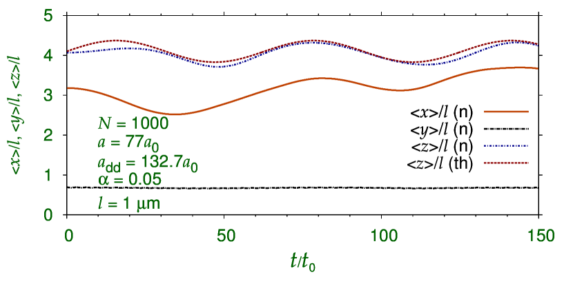
Figure 6: (Color online) Numerical (n) result for oscillation dynamics of the soliton of Fig. 2 (c) after multiplying both nonlinearities $g$ and $g_{\mathrm{dd}}$ by 1.2 at $t=0$. The theoretical (th) result for oscillation of $\langle z(t)-z(0)\rangle/l\sim\sin(2\alpha t/t_{0})$ is also shown for a comparison.

To demonstrate further the robustness of the solitons we consider a head-on collision between two solitons moving along the $x$ axis in opposite directions. We consider the collision between two identical bright solitons of Fig. 2 (c) each of 1000 ¹⁶⁴Dy atoms with $a=77a_{0}$. and $l=1$ $\mu$m. The constant velocity of about 1.9 mm/s of each of the colliding solitons was achieved by phase imprinting the wave function profiles, obtained from an imaginary-time simulation in 3D, with the factors $\exp(\pm\mathrm{i}7.5x)$. In Fig. 5 we plot the integrated 1D density $n_{1D}(x)$ for the collision dynamics obtained from Eq. (13) after a real-time numerical simulation in 3D. After the collision, the solitons emerge without a visible change of shape demonstrating the solitonic nature. However, at lower incident velocities the collision becomes inelastic and distortion in the shape of the solitons is noted.

As a further test of stability of the solitons, we demonstrate their sustained oscillation under a sizable perturbation. We perform a real-time simulation of the 3D profile of the soliton of Fig. 2 (c) upon multiplying both the nonlinearities $g$ and $g_{\mathrm{dd}}$ in Eq. (5) by the factor 1.2. The soliton executes breathing oscillation as illustrated in Fig. 6 where we plot the root-mean-square sizes $\langle x\rangle,\langle y\rangle,\langle z\rangle$, respectively, in directions $x,y$, and $z$ versus time. We also plot in this case the theoretical result for oscillation with frequency $2\alpha$ str along $z$ direction and this compares vary favorably with the numerical result.

IV Conclusion

We demonstrated the possibility of creating stable bright solitons in dipolar BEC mobile in a direction ($x$) perpendicular to the polarization direction ($z$) using the full mean-field GP equation in 3D and a reduced 2D GP equation in the plane $x-z$. The reduced 2D model is found to yield results in excellent agreement with the full 3D model. The head on collision between two identical solitons with relative velocity of about 4 mm/s is demonstrated to be quasi elastic with the solitons passing through each other with practically no deformation. The solitons are found to execute sustained breathing oscillation upon a small perturbation. The numerical simulation was done by explicitly solving the GP equation with realistic values of contact and dipolar interactions of ¹⁶⁴Dy atoms. The results and conclusions of the present paper can be tested in experiments with present-day know-how and technology and should lead to interesting future investigations.

We thank FAPESP and CNPq (Brazil) for partial support.

References

- (1) Y. S. Kivshar and B. A. Malomed, Rev. Mod. Phys. 61, 763 (1989); F. K. Abdullaev, A. Gammal, A. M. Kamchatnov, and L. Tomio, Int. J. Mod. Phys. B 19, 3415 (2005).
- (2) K. E. Strecker, G. B. Partridge, A. G. Truscott, and R. G. Hulet, Nature (London) 417, 150 (2002); L. Khaykovich, F. Schreck, G. Ferrari, T. Bourdel, J. Cubizolles, L. D. Carr, Y. Castin, and C. Salomon, Science 256, 1290 (2002).
- (3) S. L. Cornish, S. T. Thompson, and C. E. Wieman, Phys. Rev. Lett. 96, 170401 (2006).
- (4) S. Inouye et al., Nature (London) 392, 151 (1998).
- (5) M. Lu, S. H. Youn, and B. L. Lev, Phys. Rev. Lett. 104, 063001 (2010); J. J. McClelland and J. L. Hanssen, Phys. Rev. Lett. 96, 143005 (2006); S. H. Youn, M. W. Lu, U. Ray, and B. V. Lev, Phys. Rev. A 82, 043425 (2010).
- (6) M. Lu, N. Q. Burdick, Seo Ho Youn, and B. L. Lev, Phys. Rev. Lett. 107, 190401 (2011).
- (7) K. Aikawa et al., Phys. Rev. Lett. 108, 210401 (2012).
- (8) T. Lahaye et al., Nature (London) 448, 672 (2007); A. Griesmaier et al., Phys. Rev. Lett. 97, 250402 (2006).
- (9) T. Lahaye et al., Rep. Prog. Phys. 72, 126401 (2009).
- (10) L. E. Young-S., P. Muruganandam, and S. K. Adhikari, J. Phys. B 44, 101001 (2011).
- (11) R. Nath, P. Pedri, and L. Santos, Phys. Rev. Lett. 102, 050401 2009; P. Pedri and L. Santos, Phys. Rev. Lett. 95, 200404 (2005); I. I. Tikhonenkov, B. A. Malomed, and A. Vardi, Phys. Rev. Lett. 100, 090406 (2008); P. Köberle, D. Zajec, G. Wunner, and B. A. Malomed, Phys. Rev. A 85, 023630 (2012); R. Eichler, D. Zajec, P. Köberle, J. Main, and G. Wunner, Phys. Rev. A 86, 053611 (2012); R. Eichler, J. Main, and G. Wunner, Phys. Rev. A 83, 053604 (2011); Ai-Xia Zhang and Ju-Kui Xue, Phys. Rev. A 82, 013606 (2010); V. M. Lashkin, Phys. Rev. A 75, 043607 (2007).
- (12) S. K. Adhikari and P. Muruganandam, J. Phys. B 45, 045301 (2012); I. Tikhonenkov, B. A. Malomed, and A. Vardi, Phys. Rev. A 78, 043614 (2008).
- (13) S. K. Adhikari, Phys. Rev. A89, 043615 (2014).
- (14) S. K. Adhikari, J. Phys. B 47, in press (2014) arXiv:1409.5145.
- (15) S. K. Adhikari and P. Muruganandam, Phys. Lett. A 376, 2200 (2012).
- (16) S. Ronen, D. C. E. Bortolotti, and J. L. Bohn, Phys. Rev. Lett. 98, 030406 (2007).
- (17) K. Goral and L. Santos, Phys. Rev. A. 66, 023613 (2002); S. Yi and L. You, Phys. Rev. A 63, 053607 (2001).
- (18) L. Salasnich, A. Parola, and L. Reatto, Phys. Rev. A. 65, 043614 (2002).
- (19) C. Ticknor, R. M. Wilson and J. L. Bohn, Phys. Rev. Lett. 106, 065301 (2011).
- (20) R. Kishor Kumar, L. E. Young-S., D. Vudragović, A. Balaž, P. Muruganandam, S. K. Adhikari, Fortran and C programs for the time-dependent dipolar Gross-Pitaevskii equation in an anisotropic trap, submitted for publication (2014).
- (21) P. Muruganandam and S. K. Adhikari, Comput. Phys. Commun. 180, 1888 (2009); D. Vudragovic, I. Vidanovic, A. Balaz, P. Muruganandam, and S. K. Adhikari, Comput. Phys. Commun. 183, 2021 (2012); S. K. Adhikari and P. Muruganandam, J. Phys. B 35, 2831 (2002).
- (22) S. Stringari, Phys. Rev. Lett. 77, 2360 (1996).