Regularization of zero-range effective interactions in finite nuclei

Abstract

The problem of the divergences which arise in beyond mean-field calculations, when a zero-range effective interaction is employed, has not been much considered so far. Some of us have proposed, quite recently, a scheme to regularize a zero-range Skyrme-type force when it is employed to calculate the total energy, at second-order perturbation theory level, in uniform matter. Although this scheme looked promising, the extension for finite nuclei is not straightforward. We introduce such procedure in the current paper, by proposing a regularization procedure that is similar, in spirit, to the one employed to extract the so-called $V_{\rm low-k}$ from the bare force. Although this has been suggested already by B.G. Carlsson and collaborators, the novelty of our work consists in setting on equal footing uniform matter and finite nuclei; in particular, we show how the interactions that have been regularized in uniform matter behave when they are used in a finite nucleus with the corresponding cutoff. We also address the problem of the validity of the perturbative approach in finite nuclei for the total energy.

I Introduction

Self-consistent mean-field approaches provide a fairly good starting approximation to describe atomic nuclei Bender et al. (2003). Whereas so-called ab-initio approaches are increasingly successful, they cannot at present describe heavy systems and/or high-lying excited states. Mean-field approaches, instead, are able to reproduce both the experimentally observed trends of many ground-state properties (masses, radii, deformations etc.) and several features of excited states (giant resonances, rotational bands); moreover, they can be extended if needed. Either non relativistic Hamiltonians of the Skyrme or Gogny type, or covariant relativistic mean-field (RMF) Lagrangians have been used indeed beyond the mean-field approximation, for instance in second-order calculations Neck et al. (1991, 1993), in multiparticle-multihole schemes Pillet et al. (2008), in particle-vibration coupling (PVC) models Bernard and Giai (1980); Colò et al. (2010); Mizuyama et al. (2012); Mizuyama and Ogata (2012); Colò et al. (1992, 1994); Niu et al. (2012); Litvinova and Ring (2006); Litvinova and Afanasjev (2011); Afanasjev and Shawaqfeh (2011); Litvinova et al. (2008a); *LitvinovaGR1b; Litvinova et al. (2010, 2013), or within the generator coordinate method (GCM) approach Yao et al. (2013); Rodríguez and Martínez-Pinedo (2010); Nikšić et al. (2014); Yao et al. (2014).

In such approaches one introduces further correlations on top of those implicit in the mean field. Within PVC, the nucleons feel the effect of the dynamical fluctuations of the mean field, on top of its static part; within GCM, the variational space associated with a single mean-field configuration is enlarged by superimposing several mean-field configurations, each being connected with a different value of some global parameter like the quadrupole deformation. If effective interactions are fitted at mean-field level one would imagine that a re-fit of these interactions is mandatory if they are employed in a different framework. However, this is usually not done and Skyrme and Gogny forces or RMF Lagrangians are used as they are. We have in mind, for the follow-up of our discussion, mainly the PVC case since we shall consider in detail the lowest-order approximation to that model.

If single-particle (s.p.) nuclear states are calculated using Skyrme or RMF Lagrangians, the corrections induced by PVC at lowest order are typically several hundreds of keV, ranging from small values to $\approx$ 1-2 MeV Bortignon and Sagawa (2010). These corrections improve as a rule the agreement with experiment, leading to a r.m.s. deviation with respect to experimental values of about 1 MeV or less in e.g. ²⁰⁸Pb Colò et al. (2010); Cao et al. (2014). However, the convergence of these results with respect to the model space is hard to assess. Normally, one assumes that the model space is limited by the fact that only collective vibrations should be taken into account but this does not set a cutoff in a clear-cut way.

At the same time, there is another practical and yet more general point to be kept in mind. When zero-range forces are used in a beyond mean-field approach like PVC, divergences arise. In other words, diagrams beyond the HF ones (like those displayed in Fig. 1 of Colò et al. (2010)) can be shown, by simple power counting arguments, to diverge as the model space is enlarged. This is not a specific problem of Skyrme as also Gogny forces possess a zero-range term. We do not dispose at present of a reliable, fully microscopic non relativistic Hamiltonian without zero-range terms. As a consequence, it is necessary to devise a regularization technique to absorb this divergence and go beyond the usual PVC calculations. In the current work, we focus on the Skyrme case.

To simplify the formidable problem of finding a reliable regularization technique for nuclei, we only consider in the following the lowest-order (that is, second order) approximation for PVC in which the phonon is replaced by a particle-hole (p-h) pair, and we focus on the correction to the total energy instead of the correction to the s.p. energies. This problem has been already tackled in uniform matter Moghrabi et al. (2010, 2012), where it has been shown that at least a cutoff regularization is possible for a general Skyrme interaction and an arbitrary neutron/proton ratio. A dimensional regularization technique Moghrabi and Grasso (2012) has also been proposed, whereas the general study of the renormalizability of a Skyrme-type force has been recently addressed in Ref. Moghrabi and van Kolck (2013). Also these studies concern only uniform matter. The extension of the techniques introduced in Refs. Moghrabi et al. (2010, 2012) to finite nuclei is far from being straightforward and is the subject of the current paper.

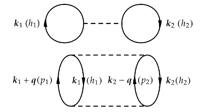
Figure 1: Diagrammatic representation of the first-order (Hartree-Fock) and second-order total energy, respectively in the upper and lower parts of the figure. The labels outside (inside) parenthesis are those used in the text for the case of uniform matter (finite nuclei).

The total energy is depicted diagrammatically in Fig. 1. We have drawn only the direct contributions but exchange terms are properly included in our calculations. The first row of the figure depicts the mean-field or Hartree-Fock (HF) total energy and the second line the second-order contribution to the same quantity. The labels outside (inside) parenthesis are momentum (generic) labels, appropriate for uniform matter (nuclei) respectively.

In the case of uniform matter, a simple power counting argument dictates that the second order contribution diverges. The simplest way to understand it is the following. The integration on momentum states is finite with respect to the hole momentum states $k_{1}$, $k_{2}$ which have the Fermi momentum $k_{F}$ as an upper limit. The center-of-mass momentum conservation leaves only one further momentum scale, which has been chosen in Refs. Moghrabi et al. (2010, 2012) to be the transferred momentum. If we label the particle states needed for the calculation of the second-order energy as $k_{3}$, $k_{4}$, the matrix elements are

$$\langle\bm{k_{3}},\bm{k_{4}}|V|\bm{k_{1}},\bm{k_{2}}\rangle=\langle\bm{k_{1}}+\bm{q},\bm{k_{2}}-\bm{q}|V|\bm{k_{1}},\bm{k_{2}}\rangle$$ (1)

(cf. Fig. 2), and the quantity

$$\bm{q}\equiv\frac{\bm{k_{3}}-\bm{k_{4}}-\bm{k_{1}}+\bm{k_{2}}}{2}$$ (2)

is the transferred momentum. For a zero-range interaction without velocity dependence (i.e., a pure $\delta$-force) the second-order contribution diverges linearly, or in other words it scales as $\int\frac{d^{3}q}{q^{2}}$, while the divergence is more severe if momentum-dependent terms are included. In Refs. Moghrabi et al. (2010, 2012) it has been shown that, by setting a cutoff $\Lambda$ on the transferred momentum, given an interaction $V$ that provides a reasonable total energy at mean-field level, it is possible to fit an interaction $V_{\Lambda}$ that reproduces the same energy when the second-order correction has been included with the cutoff $\Lambda$.

Figure 2: Representation of matrix elements in the case of uniform matter. We compare the notation used in the present paper (left) with the one in which the transferred momentum $q$ appears (right).

In finite nuclei, at variance with uniform matter, there is not translational invariance and in dealing with the matrix elements (1) we are left with two free parameters or two energy scales. In the current work we have dealt with the two scales by defining in a precise fashion the relative and center-of-mass coordinates and the associated momenta. Since the separation of center-of-mass and relative motion wave functions can be done in a neat way by using an harmonic oscillator basis, the calculations that we shall discuss below have been performed on that basis. We have systematically defined a cutoff $\lambda$ on the relative momenta (in initial and final channel) defined as

$$\bm{k} \equiv \frac{\bm{k_{1}}-\bm{k_{2}}}{\sqrt{2}},$$

$$\bm{k^{\prime}} \equiv \frac{\bm{k_{3}}-\bm{k_{4}}}{\sqrt{2}}.$$ (3)

Then, in our study, we will show how a simplified Skyrme interaction, in which only the $t_{0}$, $t_{3}$ and $\alpha$ parameters are kept and which has been regularized in uniform matter, behaves when it is used in a finite nucleus. We restrict ourselves to the case of even-even, isospin-symmetric nuclei; in particular, we will show results for ¹⁶O without Coulomb and spin-orbit forces. Our approach is thus self-consistent in the sense that we use the same Skyrme interaction both at mean-field and second order level, but we compute the total energy at second order in a perturbative way, by adding the beyond mean-field contribution on top of HF solutions. We will eventually address the problem of the validity of such perturbative approach for the total energy of a finite nucleus.

The structure of the paper is the following. Sec. II is devoted to a thorough explanation of the formalism we wish to introduce: in particular, in subsec. II.1 we discuss the interaction and its regularization, whereas in the next subsection II.2 we show the relationship between the new cutoff employed in this work and the cutoff that had been introduced previously in uniform matter. The specific formulas that implement the regularized calculation of the total energy in a finite nucleus, on the harmonic oscillator basis, are introduced in subsec. II.3. In Sec. III we describe the results obtained in the case of ¹⁶O. Conclusions and considerations related to the envisaged follow-up of this work, are in Sec. IV.

II Formalism

II.1 The regularization of the interaction

The cutoff on the relative momentum components of the effective interaction is analogous to that discussed in Ref. Carlsson et al. (2013). The underlying philosophy is the same as in the case of the $V_{\rm low-k}$ interaction and it seems quite natural, even by invoking the original argument that the Skyrme interaction is a polynomial expansion in the relative momentum that stops at second order Skyrme (1959). Therefore, we introduce the cutoffs on the relative momenta of the initial and final states and we define a regularized interaction through these cutoffs. In principle, this procedure could be avoided by using a finite-range force. However, as we stressed in the Introduction, we miss at present a widely used, reliable microscopic pure finite-range force.

To identify properly the relative momenta we introduce center-or-mass and relative coordinates. We start by writing the velocity-independent part of the Skyrme force in this form:

$$V(\bm{r}^{\prime}_{1},\bm{r}^{\prime}_{2},\bm{r}_{1},\bm{r}_{2})=g\left(\frac{\bm{r}_{1}+\bm{r}_{2}}{2}\right)\delta(\bm{r}_{1}-\bm{r}_{2})\delta(\bm{r}_{1}-\bm{r}^{\prime}_{1})\delta(\bm{r}_{2}-\bm{r}^{\prime}_{2}).$$ (4)

Our desired change of variables reads

$$\left(\begin{array}[]{l}\bm{r}^{(\prime)}\\ \bm{R}^{(\prime)}\end{array}\right)=\left(\begin{array}[]{rr}\frac{1}{\sqrt{2}}&-\frac{1}{\sqrt{2}}\\ \frac{1}{\sqrt{2}}&\frac{1}{\sqrt{2}}\\ \end{array}\right)\left(\begin{array}[]{l}\bm{r}^{(\prime)}_{1}\\ \bm{r}^{(\prime)}_{2}\end{array}\right),$$ (5)

so that the interaction (4) can be written as

$$\begin{split}V(\bm{r}^{\prime},\bm{R}^{\prime},\bm{r},\bm{R})&=\frac{\sqrt{2}}{4}g\biggl{(}\frac{\bm{R}}{\sqrt{2}}\biggr{)}\delta(\bm{r})\delta(\bm{r}^{\prime})\delta(\bm{R}-\bm{R}^{\prime})\\ &=\frac{\sqrt{2}}{4}g\biggl{(}\frac{\bm{R}}{\sqrt{2}}\biggr{)}v(\bm{r}^{\prime},\bm{r})\delta(\bm{R}-\bm{R}^{\prime}),\end{split}$$ (6)

where $g(\bm{R})=t_{0}+\frac{t_{3}}{6}\left[\rho\left(\bm{R}\right)\right]^{\alpha}$. The Fourier transform of the interaction can be written in a straightforward way as

$$\begin{split}V\left(\bm{k}_{3},\bm{k}_{4},\bm{k}_{1},\bm{k}_{2}\right)=\frac{\sqrt{2}}{4}&\frac{1}{\Omega}\int\mathrm{d}^{3}R\mathrm{d}^{3}R^{\prime}\,\mathrm{e}^{-i\frac{\bm{k}_{3}+\bm{k}_{4}}{\sqrt{2}}\!\cdot\!\bm{R}^{\prime}}g\biggl{(}\frac{\bm{R}}{\sqrt{2}}\biggr{)}\delta\left(\bm{R}-\bm{R}^{\prime}\right)\mathrm{e}^{i\frac{\bm{k}_{1}+\bm{k}_{2}}{\sqrt{2}}\!\cdot\!\bm{R}}\times\\ \times&\frac{1}{\Omega}\int\mathrm{d}^{3}r\mathrm{d}^{3}r^{\prime}\,\mathrm{e}^{-i\frac{\bm{k}_{3}-\bm{k}_{4}}{\sqrt{2}}\!\cdot\!\bm{r}^{\prime}}v(\bm{r}^{\prime},\bm{r})\mathrm{e}^{i\frac{\bm{k}_{1}-\bm{k}_{2}}{\sqrt{2}}\!\cdot\!\bm{r}},\end{split}$$ (7)

by introducing a finite quantization volume $\Omega$. The factor appearing in the second line of this equation can be written in terms of the variables $\bm{k}\equiv\frac{\bm{k}_{1}-\bm{k}_{2}}{\sqrt{2}}$ and $\bm{k}^{\prime}\equiv\frac{\bm{k}_{3}-\bm{k}_{4}}{\sqrt{2}}$ that are the conjugate variables of the relative coordinates defined by Eq. (5): these are the relative momenta (of the initial and final state respectively) that we have already introduced in Eq. (3). Thus we re-write the factor in the second line of Eq. (7) as

$$v(\bm{k}^{\prime},\bm{k}) =\frac{1}{\Omega}\int\mathrm{d}^{3}r\mathrm{d}^{3}r^{\prime}\,\mathrm{e}^{-i\bm{k}^{\prime}\!\cdot\bm{r}^{\prime}}v(\bm{r}^{\prime},\bm{r})\mathrm{e}^{i\bm{k}\!\cdot\bm{r}}=\frac{1}{\Omega},$$ (8)

where the last equality obviously holds if $v(\bm{r}^{\prime},\bm{r})=\delta(\bm{r})\delta(\bm{r}^{\prime})$ as we have written in Eq. (6) (we will keep this notation in what follows).

Then, we introduce the regularized interaction as the inverse Fourier transform of (8) in which two step functions $\theta(\lambda-k)\theta(\lambda^{\prime}-k^{\prime})$ are introduced. In this way, $\lambda$ and $\lambda^{\prime}$ are the cutoffs in the relative momenta $\bm{k}$ and $\bm{k^{\prime}}$, respectively, and the regularized interaction $v^{\lambda\lambda^{\prime}}$ is obtained as

$$v^{\lambda\lambda^{\prime}}(\bm{r}^{\prime},\bm{r})= \frac{1}{\Omega}\int\mathrm{d}^{3}k\mathrm{d}^{3}k^{\prime}\,\mathrm{e}^{i\bm{k}^{\prime}\!\cdot\bm{r}^{\prime}}v\left(\bm{k}^{\prime},\bm{k}\right)\theta(\lambda-k)\theta(\lambda^{\prime}-k^{\prime})\mathrm{e}^{-i\bm{k}\!\cdot\bm{r}}$$

$$= \frac{1}{4\pi^{4}}\frac{\lambda^{2}\lambda^{\prime 2}}{rr^{\prime}}j_{1}(r\lambda)j_{1}(r^{\prime}\lambda^{\prime})\xrightarrow[\begin{subarray}{c}\lambda\rightarrow+\infty\\ \lambda^{\prime}\rightarrow+\infty\end{subarray}]{}\delta(\bm{r})\delta(\bm{r}^{\prime}),$$ (9)

where the usual expansion of the plane waves in spherical components is used, and the limit in the last line comes from Eq. (3.5) of Ref. Mehrem (2011).

In what follows, we will employ the regularized interaction $v^{\lambda\lambda^{\prime}}(\bm{r}^{\prime},\bm{r})$ to evaluate the matrix elements of the interaction (6), and at times compare with the matrix elements obtained by using the bare interaction $v(\bm{r}^{\prime},\bm{r})$.

II.2 Uniform matter and the different choices for the cutoff

In this subsection, we wish to establish a connection between the cutoff on the transferred momentum (2) Moghrabi et al. (2010, 2012) and the cutoff on the relative momenta (3). At the same time, we deal in this subsection with that fact that in the procedure adopted in Refs. Moghrabi et al. (2010, 2012) there is no cutoff affecting the HF energy. In the present scheme, we introduce a cutoff consistently in the HF and second-order energies.

The HF potential energy, shown diagrammatically in the upper part of Fig. 1, is

$$E_{\rm HF}=\frac{1}{2}\sum_{ij}\langle ij|\bar{V}|ij\rangle,$$ (10)

where $\bar{V}$ is the antisymmetrized interaction. If we write the HF energy in symmetric nuclear matter as in Ref. Moghrabi et al. (2010), we obtain

$$\frac{E}{A}=8\frac{dgk_{F}^{6}}{\rho(2\pi)^{6}}\frac{4\pi}{3}\int\mathrm{d}^{3}\tilde{k}\,\left(1-\frac{3}{2}\tilde{k}+\frac{1}{2}\tilde{k}^{3}\right)\theta(1-\tilde{k})=\frac{3}{8}g\rho,$$ (11)

where $d$ is the level degeneracy (4 in the case of symmetric nuclear matter) and $\tilde{\bm{k}}$ is defined only in this subsection, for the sake of convenience, as $\tilde{\bm{k}}\equiv{\bm{k}}/\sqrt{2}k_{F}$. If we now wish to introduce the cutoff $\lambda$ on $\bm{k}$, we have to add a factor $\theta\!\left(\frac{\lambda}{\sqrt{2}k_{F}}-\tilde{k}\right)$. Then, Eq. (11) becomes

$$\frac{E}{A}=8\frac{dgk_{F}^{6}}{\rho(2\pi)^{6}}\frac{4\pi}{3}\int\mathrm{d}^{3}\tilde{k}\,\left(1-\frac{3}{2}\tilde{k}+\frac{1}{2}\tilde{k}^{3}\right)\theta(1-\tilde{k})\theta\!\left(\frac{\lambda}{\sqrt{2}k_{F}}-\tilde{k}\right)=\frac{3}{8}g\rho\left(8\beta^{3}-9\beta^{4}+2\beta^{6}\right),$$ (12)

where $\beta=\min\{1,\frac{\lambda}{\sqrt{2}k_{F}}\}$. Clearly, if $\lambda>\sqrt{2}k_{F}$, then $\beta=1$ and we recover the result of Eq. (11). This has been tested also numerically, and the result is displayed in Fig. 3. Note the similar figure and reasoning in Ref. Carlsson et al. (2013).

Figure 3: (Color online) Energy per particle at the HF level [cf. Eqs. (10,12)] for different values of the cutoff $\lambda$ on the relative momentum $\bm{k}$.

As for the second order contribution to the total energy, the relation between momenta used in the present work and those employed previously Moghrabi et al. (2010, 2012) can be written, generalizing Eq. (3), as

$$\left(\begin{array}[]{l}\bm{k}\\ \bm{k}^{\prime}\\ \bm{k}^{\prime\prime}\end{array}\right)=\left(\begin{array}[]{rrr}\frac{1}{\sqrt{2}}&-\frac{1}{\sqrt{2}}&0\\ \frac{1}{\sqrt{2}}&-\frac{1}{\sqrt{2}}&\sqrt{2}\\ \frac{1}{\sqrt{2}}&\frac{1}{\sqrt{2}}&0\\ \end{array}\right)\left(\begin{array}[]{l}\bm{k}_{1}\\ \bm{k}_{2}\\ \bm{q}\end{array}\right).$$ (13)

The determinant of the Jacobian matrix of this transformation is 1. One can note that

$${\bm{k}^{\prime}}={\bm{k}}+\sqrt{2}{\bm{q}}.$$ (14)

The second order contribution to the total energy, displayed in the lower part of Fig. 1 with diagrams, is

$$\Delta E=\frac{1}{2}\sum_{ijmn}\frac{\langle mn|V|ij\rangle\langle ij|\bar{V}|mn\rangle}{\varepsilon_{i}+\varepsilon_{j}-\varepsilon_{m}-\varepsilon_{n}},$$ (15)

where $\varepsilon$ are HF s.p. energies. We evaluate this expression in symmetric matter and we keep the notation of this subsection, that is, $\tilde{\bm{k}}\equiv{\bm{k}}/\sqrt{2}k_{F}$ and $\tilde{\bm{k}}^{\prime}\equiv{\bm{k}}^{\prime}/\sqrt{2}k_{F}$, $\tilde{\bm{k}}^{\prime\prime}\equiv{\bm{k}}^{\prime\prime}/\sqrt{2}k_{F}$ in an analogous way. Thus, we obtain

$$\frac{\Delta E}{A}=\chi(\rho)\frac{\sqrt{2}}{4\pi^{3}}\int_{\mathcal{D}(\tilde{\bm{k}},\tilde{\bm{k}}^{\prime},\tilde{\bm{k}}^{\prime\prime})}\mathrm{d}^{3}\tilde{k}\mathrm{d}^{3}\tilde{k}^{\prime}\mathrm{d}^{3}\tilde{k}^{\prime\prime}\,\frac{1}{\tilde{k}^{\prime 2}-\tilde{k}^{2}},$$ (16)

where $\chi(\rho)$ has been defined in Ref. Moghrabi et al. (2010), and the domain of integration is

$$\mathcal{D}(\tilde{\bm{k}},\tilde{\bm{k}}^{\prime},\tilde{\bm{k}}^{\prime\prime})\equiv\biggl{\{}\tilde{\bm{k}},\tilde{\bm{k}}^{\prime},\tilde{\bm{k}}^{\prime\prime}\in\mathbb{R}^{3}\colon\tilde{k}\leq 1,\tilde{k}^{\prime\prime}\leq 1,\left(\left|\tilde{\bm{k}}^{\prime\prime}+\tilde{\bm{k}}\right|<1\cap\left|\tilde{\bm{k}}^{\prime\prime}-\tilde{\bm{k}}\right|<1\right)\cup\left(\left|\tilde{\bm{k}}^{\prime\prime}+\tilde{\bm{k}}^{\prime}\right|>1\cap\left|\tilde{\bm{k}}^{\prime\prime}-\tilde{\bm{k}}^{\prime}\right|>1\right)\biggr{\}}.$$

Our purpose is now to compare with the results of Ref. Moghrabi et al. (2010) and convince ourselves that we can use the interactions that have been fitted therein. To this aim, we must consider the case in which the cutoff $\lambda$ on relative momenta is larger than $\sqrt{2}k_{F}$, since otherwise the HF energy should be also modified compared to the calculation with the bare force performed in Ref. Moghrabi et al. (2010) (cf. above). On top of this, the calculation of the integral appearing in Eq. (16) is rather cumbersome, and can be slightly simplified if $\lambda$ is larger than $2\sqrt{2}k_{F}$. In this case a detailed analytic evaluation has been carried out Brenna (2014). The result can be written as

$$\begin{split}\frac{\Delta E}{A}=\chi(\rho)\biggl{\{}&-\frac{11}{105}+\frac{2}{105}\ln{2}+\frac{2}{35}\tilde{\lambda}-\frac{11}{35}\tilde{\lambda}^{3}-\frac{2}{21}\tilde{\lambda}^{5}-\left(\frac{4\tilde{\lambda}^{5}}{5}-\frac{4\tilde{\lambda}^{7}}{21}\right)\ln\left(\tilde{\lambda}\right)\\ &+\left(\frac{1}{35}-\frac{\tilde{\lambda}^{4}}{3}+\frac{2\tilde{\lambda}^{5}}{5}-\frac{2\tilde{\lambda}^{7}}{21}\right)\ln\left(\tilde{\lambda}-1\right)-\left(\frac{1}{35}-\frac{\tilde{\lambda}^{4}}{3}-\frac{2\tilde{\lambda}^{5}}{5}+\frac{2\tilde{\lambda}^{7}}{21}\right)\ln\left(\tilde{\lambda}+1\right)\biggr{\}},\end{split}$$ (17)

where $\tilde{\lambda}\equiv\frac{\lambda}{\sqrt{2}k_{F}}$. We have checked that the part that does not depend on $\lambda$ is equal to the one already written in Ref. Moghrabi et al. (2010), as it should, and that the divergence is linear.

To obtain a better understanding, we have evaluated numerically the two results given by Eq. (17) and Eq. (8) of Ref. Moghrabi et al. (2010). The two calculations are almost indistinguishable when

$$\lambda=\sqrt{2}\Lambda.$$ (18)

We will then use this latter equation in the following way: when we perform a calculation of a finite system with cutoff $\lambda$ we will adopt the interaction fitted in uniform symmetric matter with the value of $\lambda$ given by Eq. (18). Ultimately, we would envisage to cast uniform matter and finite nuclei in a single scheme, so to be able to fit an effective force in the same spirit of the original Skyrme force (at second order and then beyond).

II.3 The formalism for finite nuclei using the harmonic oscillator basis

In finite nuclei the second order energy is still given by Eq. (15) but is more conveniently written in angular momentum-coupled representation as

$$\Delta E=\frac{1}{4}\sum_{pp^{\prime}hh^{\prime}J}\frac{(2J+1)|\langle(pp^{\prime})J|\bar{V}|(hh^{\prime})J\rangle|^{2}}{\varepsilon_{h}+\varepsilon_{h^{\prime}}-\varepsilon_{p}-\varepsilon_{p^{\prime}}},$$ (19)

where the particle-particle (pp) coupled matrix elements have been introduced, namely

$$\begin{aligned} \langle(\alpha\beta)J&M_{J}|\bar{V}|(\gamma\delta)JM_{J}\rangle=\sum_{\begin{subarray}{c}m_{\alpha}m_{\beta}\\ m_{\gamma}m_{\delta}\end{subarray}}\langle j_{\alpha}m_{\alpha}j_{\beta}m_{\beta}|JM_{J}\rangle\langle j_{\gamma}m_{\gamma}j_{\delta}m_{\delta}|JM_{J}\rangle\langle\alpha\beta|\bar{V}|\gamma\delta\rangle\\ &=\sum_{\begin{subarray}{c}m_{\alpha}m_{\beta}\\ m_{\gamma}m_{\delta}\end{subarray}}(-)^{j_{\alpha}-j_{\beta}+j_{\gamma}-j_{\delta}}\hat{J}^{2}\begin{pmatrix}j_{\alpha}&j_{\beta}&J\\ m_{\alpha}&m_{\beta}&-M_{J}\end{pmatrix}\begin{pmatrix}j_{\gamma}&j_{\delta}&J\\ m_{\gamma}&m_{\delta}&-M_{J}\end{pmatrix}\langle\alpha\beta|\bar{V}|\gamma\delta\rangle,\end{aligned}$$ (20)

where we have introduced the common shorthand notation $\hat{J}^{2}=2J+1$. Actually, these latter matrix elements do not depend on $M_{J}$ because of rotational invariance. Therefore, in Eq. (19) they appear without this label; in that equation, the trivial sum over $M_{J}$ has been performed.

In our calculation, we expand the single-particle wave functions in harmonic oscillator basis. Then, the corresponding matrix elements are evaluated by performing the transformation of the initial and final two-particle states to the center of mass and relative motion coordinates. As is well known, this can be done in the HO case by exploiting the Brody-Moshinsky transformations Lawson (1980); Buck and Merchant (1996); Kamuntavičius et al. (2001). In this subsection we will collect only the main equations related to the matrix elements entering our calculations; we shall provide some more details about the main steps of their derivation, together with other useful formulas, in the Appendix.

We shall indicate with the label $I$ = $0$, $\sigma$, $\tau$ and $\sigma\tau$ the terms of the pp-coupled matrix elements (20) that are proportional, respectively, to the identity in spin-isospin space, to $\bm{\sigma}(1)\bm{\sigma}(2)$, to $\bm{\tau}(1)\bm{\tau}(2)$ and to $\bm{\sigma}(1)\bm{\sigma}(2)\ \bm{\tau}(1)\bm{\tau}(2)$. The final expression for these terms reads

$$\langle(n_{a}l_{a} j_{a}\tau_{a},n_{b}l_{b}j_{b}\tau_{b})JM_{J}|\bar{V}|(n_{c}l_{c}j_{c}\tau_{c},n_{d}l_{d}j_{d}\tau_{d})JM_{J}\rangle_{I}=$$

$$= \mathcal{N}_{I}\mathcal{F}_{I}\sum_{\Sigma L}i^{-l_{a}-l_{b}+l_{c}+l_{d}}\hat{L}^{2}\hat{\Sigma}^{2}\hat{j}_{a}\hat{j}_{b}\hat{j}_{c}\hat{j}_{d}\mathcal{G}_{I}\begin{Bmatrix}l_{a}&l_{b}&L\\ \frac{1}{2}&\frac{1}{2}&\Sigma\\ j_{a}&j_{b}&J\end{Bmatrix}\begin{Bmatrix}l_{c}&l_{d}&L\\ \frac{1}{2}&\frac{1}{2}&\Sigma\\ j_{c}&j_{d}&J\end{Bmatrix}$$

$$\frac{\lambda^{2}\lambda^{\prime 2}}{\pi^{3}}\sum_{\begin{subarray}{c}n_{i}N_{i}\\ n_{f}N_{f}\end{subarray}}M_{L}(N_{f}Ln_{f}0;n_{a}l_{a}n_{b}l_{b})M_{L}(N_{i}Ln_{i}0;n_{c}l_{c}n_{d}l_{d})$$ (21)

$$\int\mathrm{d}RR^{2}R_{N_{f}L}(\sqrt{2}\beta R)g(R)R_{N_{i}L}(\sqrt{2}\beta R)$$

$$\int\mathrm{d}r\,rR_{n_{i}0}(\beta r)j_{1}(r\lambda)\int\mathrm{d}r^{\prime}\,r^{\prime}R_{n_{f}0}(\beta r^{\prime})j_{1}(r^{\prime}\lambda^{\prime}).$$

Here the single-particle states are labelled by the usual quantum numbers in spherical symmetry, $n,l,j$, together with the third component of the isospin $\tau$. These single-particle states are expanded in the harmonic oscillator basis, and $\beta$ is the harmonic oscillator parameter, $\beta\equiv\sqrt{m\omega/\hbar}$. The harmonic oscillator single-particle states and their radial wave functions $R$ are defined in Eq. (27). The symbol $M_{L}$ corresponds to the Brody-Moshinsky coefficients. The quantities $\mathcal{N}_{I},\mathcal{F}_{I},\mathcal{G}_{I}$ are defined in the Appendix. Although the structure of the formula should look clear, as it includes the transformations (i) to $LS$-coupling, (ii) to the harmonic oscillator basis, (ii) to the center-of-mass and relative coordinates, reading the Appendix may shed some further light on it.

The two-body matrix elements (21) constitute the backbone of our calculation. Nonetheless, since as explained above we will also use the renormalized interaction at the mean field level, it is useful to provide in this subsection the final form of the one-body matrix elements of the HF Hamiltonian, that are

$$h^{(\alpha)}_{ab} =\,\,t_{ab}$$ (22)

$$+\sum_{{\begin{subarray}{c}\beta\\ \varepsilon_{\beta}\leq\varepsilon_{F}\end{subarray}}}\sum_{cd}c_{\beta,c}^{*}\langle ac|\bar{V}|bd\rangle c_{\beta,d}$$ (23)

$$+\frac{1}{2}\sum_{{\begin{subarray}{c}\beta\gamma\\ \varepsilon_{\beta,\gamma}\leq\varepsilon_{F}\end{subarray}}}\,\,\,\sum_{{cdef}}c_{\beta,c}^{*}c_{\gamma,d}^{*}\langle cd|\frac{\partial{\bar{V}}}{\partial c_{\alpha,a}^{*}}|ef\rangle c_{\beta,e}c_{\gamma,f},$$ (24)

where $c$ denotes the expansion coefficients of the s.p. states on the harmonic oscillator basis, the Greek letters represent the set of quantum number which identify a s.p. state and the Latin letters indicate the harmonic oscillator basis quantum number.

The explicit expression for the term (22) can be easily found in Ref. Bertsch (1972). The second term (23) can be written using Eq. (21). Nevertheless, the expression can be further simplified because of two simple considerations Vautherin and Brink (1972):

• we are dealing with even-even nuclei, thus the matrix elements of the operator $\bm{\sigma}(1)\bm{\sigma}(2)$ vanishes;

• there is no charge mixing of the HF states, so the isospin exchange operator $P_{\tau}$ reduces to a Kronecker delta.

With these simplifications and by using the orthogonality relations for the 9$-j$ symbol, we get

$$\sum_{{\begin{subarray}{c}\beta\\ \varepsilon_{\beta}\leq\varepsilon_{F}\end{subarray}}} \sum_{cd}c_{\beta,c}^{*}\langle ac|\bar{V}|bd\rangle c_{\beta,d}=\sum_{{\begin{subarray}{c}\beta\\ \varepsilon_{\beta}\leq\varepsilon_{F}\end{subarray}}}\sum_{cd}\sum_{J}\frac{\hat{J}^{2}}{\hat{j}^{2}_{\alpha}}c_{\beta,c}^{*}\langle(ac)JM|\bar{V}|(bd)JM\rangle c_{\beta,d}$$

$$= \sum_{{\begin{subarray}{c}\beta\\ \varepsilon_{\beta}\leq\varepsilon_{F}\end{subarray}}}\sum_{cd}c_{\beta,c}^{*}c_{\beta,d}\sum_{L}\sum_{\begin{subarray}{c}n_{i}N_{i}\\ n_{f}N_{f}\end{subarray}}\frac{\hat{L}^{2}\hat{j}^{2}_{\beta}}{\hat{l}^{2}_{\alpha}\hat{l}^{2}_{\beta}}M_{L}(N_{f}Ln_{f}0;al_{\alpha}cl_{\beta})M_{L}(N_{i}Ln_{i}0;bl_{\alpha}dl_{\beta})$$

$$\qquad\times\left(1-\frac{1}{2}\delta_{q_{\alpha},q_{\beta}}\right)\int\mathrm{d}RR^{2}R_{N_{f}L}(\sqrt{2}\beta R)g(R)R_{N_{i}L}(\sqrt{2}\beta R)$$ (25)

$$\qquad\times\frac{\lambda^{2}\lambda^{\prime 2}}{\pi^{3}}\int\mathrm{d}r\,rR_{n_{i}0}(\beta r)j_{1}(r\lambda)\int\mathrm{d}r^{\prime}\,r^{\prime}R_{n_{f}0}(\beta r^{\prime})j_{1}(r^{\prime}\lambda^{\prime}).$$

Following the same strategy, the last term (24), which is the rearrangement term, can be written as

$$\frac{1}{2}\sum_{{\begin{subarray}{c}\beta\gamma\\ \varepsilon_{\beta,\gamma}\leq\varepsilon_{F}\end{subarray}}}\,\,\, \sum_{\begin{subarray}{c}cd\\ ef\end{subarray}}c_{\beta,c}^{*}c_{\gamma,d}^{*}\langle cd|\frac{\partial{\bar{V}}}{\partial c_{\alpha,a}^{*}}|ef\rangle c_{\beta,e}c_{\gamma,f}$$

$$= \frac{1}{2}\sum_{{\begin{subarray}{c}\beta\gamma\\ \varepsilon_{\beta,\gamma}\leq\varepsilon_{F}\end{subarray}}}\,\,\,\sum_{\begin{subarray}{c}cd\\ ef\end{subarray}}c_{\beta,c}^{*}c_{\gamma,d}^{*}c_{\beta,e}c_{\gamma,f}$$

$$\times\sum_{L}\sum_{\begin{subarray}{c}n_{i}N_{i}\\ n_{f}N_{f}\end{subarray}}\frac{\hat{L}^{2}\hat{j}^{2}_{\gamma}\hat{j}^{2}_{\beta}}{\hat{l}^{2}_{\gamma}\hat{l}^{2}_{\beta}}M_{L}(N_{f}Ln_{f}0;cl_{\beta}dl_{\gamma})M_{L}(N_{i}Ln_{i}0;el_{\beta}fl_{\gamma})$$

$$\qquad\times\left(1-\frac{1}{2}\delta_{q_{\gamma},q_{\beta}}\right)\int\mathrm{d}RR^{2}R_{N_{f}L}(\sqrt{2}\beta R)g^{\prime}(R)R_{N_{i}L}(\sqrt{2}\beta R)$$ (26)

$$\qquad\times\frac{\lambda^{2}\lambda^{\prime 2}}{\pi^{3}}\int\mathrm{d}r\,rR_{n_{i}0}(\beta r)j_{1}(r\lambda)\int\mathrm{d}r^{\prime}\,r^{\prime}R_{n_{f}0}(\beta r^{\prime})j_{1}(r^{\prime}\lambda^{\prime}),$$

where $g^{\prime}(R)=\frac{t_{3}\alpha}{24\pi}R_{al_{\alpha}}(\beta R)R_{bl_{\alpha}}(\beta R)\rho^{\alpha-1}(R)$.

Table 1: Parameter sets (named SkP_Λ) obtained in the fits associated with different values of the cutoff $\Lambda$ compared with the original set SkP, labeled with SkP (first line) Moghrabi .

	$t_{0}$	$t_{3}$	$\alpha$			$t_{0}$	$t_{3}$	$\alpha$
SkP	$-$2931.70	18709.00	$1/6$
SkP0.1	$-$2937.45	18758.12	0.16674		SkP1.9	$-$649.68	7431.97	1.13340
SkP0.2	$-$2931.54	18723.70	0.16713		SkP2.0	$-$618.70	7062.93	1.16305
SkP0.3	$-$2906.45	18577.75	0.16881		SkP2.1	$-$593.41	6596.73	1.16744
SkP0.4	$-$2842.25	18204.63	0.17328		SkP2.2	$-$573.43	6052.99	1.14457
SkP0.5	$-$2719.66	17494.17	0.18249		SkP2.3	$-$558.79	5469.05	1.09369
SkP0.6	$-$2531.08	16406.95	0.19873		SkP2.4	$-$549.99	4892.54	1.01547
SkP0.7	$-$2288.58	15022.28	0.22432		SkP2.5	$-$548.24	4374.67	0.91252
SkP0.8	$-$2020.60	13517.37	0.26140		SkP3.0	$-$544.99	3624.67	0.66267
SkP0.9	$-$1758.46	12085.78	0.31144		SkP3.5	$-$514.79	3386.33	0.62361
SkP1.0	$-$1524.15	10862.96	0.37503		SkP4.0	$-$489.40	3180.44	0.59654
SkP1.1	$-$1326.93	9904.53	0.45153		SkP5.0	$-$448.19	2858.89	0.56329
SkP1.2	$-$1166.61	9204.84	0.53904		SkP8.0	$-$368.24	2279.23	0.52259
SkP1.3	$-$1038.29	8724.34	0.63454		SkP10.0	$-$334.14	2045.30	0.51106
SkP1.4	$-$935.83	8409.46	0.73409		SkP20.0	$-$244.47	1457.29	0.49046
SkP1.5	$-$853.56	8203.44	0.83327		SkP40.0	$-$176.94	1035.19	0.48119
SkP1.6	$-$786.87	8050.45	0.92736		SkP60.0	$-$145.95	846.69	0.47822
SkP1.7	$-$732.24	7899.09	1.01172		SkP80.0	$-$127.16	733.92	0.47675
SkP1.8	$-$687.11	7704.42	1.08184		SkP100.0	$-$114.20	656.81	0.47589

III Results

In our work we have focused on the calculation of the total energy (19) in ¹⁶O. As explained in the previous Sections, we aim at using interactions fitted with a cutoff regularization in uniform matter and check that this strategy is enough to prevent the divergence of the total energy in the finite system. The relation between the cutoffs that are used throughout our procedure has been given in Eq. (18) above, and reads

$$\lambda=\sqrt{2}\Lambda.$$

The interactions $V_{\Lambda}$ associated with the re-fit of symmetric matter, when the second-order contribution has an associated cutoff $\Lambda$, are provided in Table 1. As already mentioned, we employ an harmonic oscillator basis. The oscillator parameter $\beta\equiv\sqrt{m\omega/\hbar}$ is 0.5 fm^-1 and the number of oscillator shells is $n_{\rm max}$ = 10. The radial wave functions are calculated up to a maximum value of $r$ given by $R$ = 12 fm.

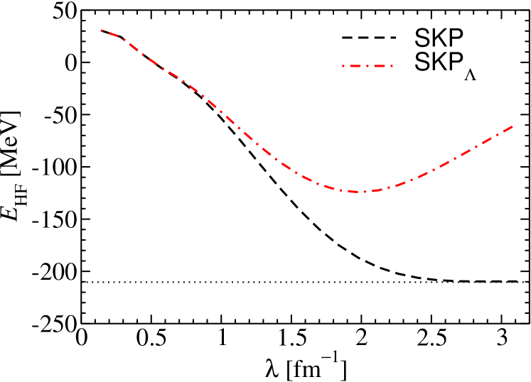
Figure 4: (Color online) Total HF energy as a function of a cutoff $\lambda$. The dashed (dot-dashed) curve corresponds to the result obtained with SkP with only $t_{0}$, $t_{3}$ terms (SkP_Λ). The thin dotted line corresponds to the result without any cutoff, obtained with SkP with only $t_{0}$, $t_{3}$ term, and is meant to guide the eye for the convergence of the dashed line. See the text for a more detailed discussion.

In Fig. 4 we display the mean-field energy obtained with the renormalized interactions, as a function of $\lambda$, by means of the line labeled with SkP_Λ. As a reference we provide the same quantity calculated with the bare interaction SkP (line labeled with SkP), and the mean field value (without cutoff) which is associated with the horizontal line and is $-210.3$ MeV. We stress here that the velocity-dependent terms of the original SkP interaction have been dropped. The original SkP set, if of course all terms (central terms, both velocity-independent but also velocity-dependent ones, spin-orbit term and Coulomb term) are retained, reasonably reproduces the experimental value of the binding energy of ¹⁶O which is known to be $-127.619$ MeV Audi et al. (2012). The HF result obtained with SkP can be understood, since when the cutoff increases the calculation tends obviously to the exact one, while reducing the momentum components amounts to trying to minimize the energy in a Hilbert space which is not complete: although the variational principle cannot be rigorously invoked, it is plausible that the energy does not attain its minimum and is instead smaller in absolute value. It is instructive to note that the convergence to the exact result is obtained only for $\lambda$ of the order of 2.5 fm^-1: in fact, inside this light nucleus the density can rise up to 0.25 fm^-3 (cf. Fig. 5) and the associated maximum effective (local) $k_{F}$ is therefore $\approx$ 1.54 fm^-1, so that the maximum value for the momenta defined in Eq. (3) can be as high as 2.2 fm^-1. The result associated with the renormalized interaction is more subtle to understand. For low values of the cutoff energy the renormalization of the interaction is not significant (as one can notice from the values of the parameters in Table 1). This is understandable, since for small values of $\lambda$ the second-order contribution in infinite matter is small, and one needs to weakly renormalize the interaction in order to obtain in the same system the HF energy associated with the bare interaction. As a consequence, for small values of $\lambda$ the curves associated with the bare and renormalized interactions overlap. However, for large values of $\lambda$ the total energy still decreases in absolute value when it is calculated with the renormalized interaction. In this case, in fact, most of the momentum components are retained, but the interaction is strongly renormalized (again, this can be seen from the values of the parameters in Table 1) and, as a consequence, the mean-field total energy is small. As a conclusion, we infer from Fig. 4 that for either too small or too large values of $\lambda$ the system calculated at mean-field level with the renormalized interaction is far away from the system we would like to reproduce by adding the second-order contribution: in other words, perturbation theory is doomed to fail for those values of $\lambda$, especially if we start from a situation in which the total energy is positive at mean-field but not only in that case. In practice, we restrict our following discussion to, and draw conclusions from, values of $\lambda$ between $\approx$ 2 and 2.7 fm^-1 (although we will show in the figures some results associated with a broader range of values for $\lambda$).

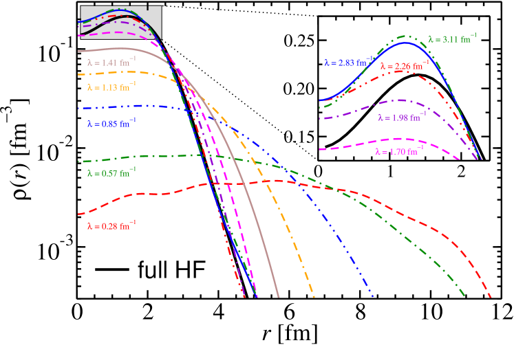
Figure 5: (Color online) Total density profiles obtained with the renormalized SkP_Λ interactions. The thick black line refers to the bare interaction. The inset shows some detail of the region in which the density attains its largest values.

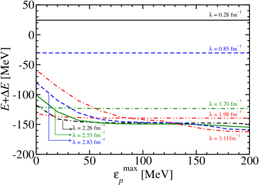
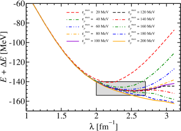
Figure 6: (Color online) Total energy at second order as a function of the maximum particle energy (left panel) or as a function of the cutoff (right panel). All curves are obtained with renormalized interactions. See the text for a discussion.

This view is in part confirmed by the results shown in Fig. 5: here we display the different profiles for the total density emerging from the HF calculations when different renormalized interactions are employed. Along the same line of the discussion in the previous paragraph, if the cutoff is small a large fraction of the high momentum or small distance components of the relative motion are cut, and the system becomes very dilute, almost like a uniform unbound nucleon gas.

We now discuss our main results, that are summarized in the three panels of Figs. 6 and 7. In the left panel of Fig. 6, the total energy calculated at second order with the renormalized interactions is shown, for various values of $\lambda$, as a function of the maximum particle energy $\varepsilon_{p}^{\rm max}$. For the sake of clarity only a selection of the results obtained with the interactions associated with different values of $\Lambda$ are displayed. For values of $\lambda$ between $\approx$ 2 and 2.7 fm^-1, the results are close to one another. Even more importantly, these results do not depend on the value of $\varepsilon_{p}^{\rm max}$, at least if this is larger than $\approx$ 80 MeV. This can be understood on the basis of a simple semiclassical argument: particles having energies larger than $\approx$ 80 MeV, and having thus very large kinetic energies, would contribute to the total energy through matrix elements associated with momentum components that are actually eliminated by our choice of the cutoff. Therefore, the most important conclusion is that our proposed renormalization procedure can work, and the extra scale associated with the maximum value of the particle energy, or with the total momentum, does not spoil that procedure.

The stability of the renormalized results for the second order energy, is also visible in the right panel of Fig. 6. The curves associated with values of $\lambda$ between $\approx$ 2 and 2.7 fm^-1, for a broad range of values of $\varepsilon_{p}^{\rm max}$, lie in the shaded box that corresponds to $\approx$ 10% error in the total energy. A quick glance of the behavior of our results is allowed by the plot of Fig. 7, that collects the same information already provided in the two panels of Fig. 6 by means of a more intuitive three-dimensional global representation.

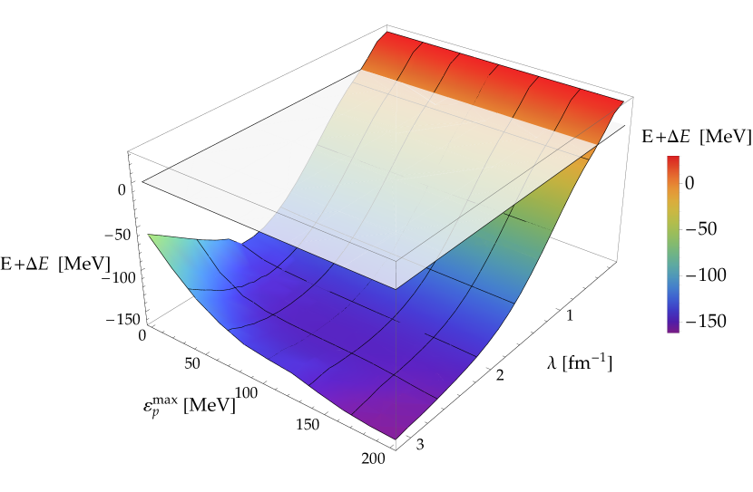
Figure 7: (Color online) The same as Fig. 6 in a three-dimensional representation, that is, total energy at second order as a function of both the maximum particle energy and the cutoff.

IV Conclusions

The problem associated with the fact that zero-range forces produce divergent results when employed beyond mean-field has become object of a renewed interest. Skyrme forces have zero-range character but also Gogny forces possess a zero-range terms; pure finite-range forces have not been so widely developed and systematically applied in non-relativistic approaches.

The problem of the renormalization of these divergences has been tackled first in a simple system like uniform nuclear matter, restricting to the case of the second-order correction to the energy. The purpose of this work is to make a significant first step in the direction of a full renormalization scheme for the Skyrme force in finite nuclei. Our main idea is to work in a harmonic oscillator basis, so that the center-of mass and relative motion coordinates and associated momenta can be neatly separated. The cutoff we set on the momentum associated with the relative motion can be then related to the one used in the previous calculations of nuclear matter. We have illustrated such formal scheme in full detail in this paper.

As a numerical application, we have limited ourselves to ¹⁶O calculated with a simple, momentum-independent Skyrme force. Our main results are listed as follows:

• under certain conditions, it is possible to relate the cutoff $\lambda$ on the relative momentum to the cutoff $\Lambda$ that has been previously introduced in Moghrabi et al. (2010, 2012) [cf. Eq. (18) and the related discussion];

• if calculations of the total energy at second order are envisaged, with a cutoff $\lambda$, the interactions introduced in uniform matter using the associated value of $\Lambda$ can be employed;

• the practical way to do these calculations is to work in harmonic oscillator basis and change the form of the interaction so that relative-momentum components larger than $\lambda$ are cut;

• at least for a reasonable range of values, $\lambda\approx 2-2.7$ fm^-1, the results turn out to be stable, namely the divergence does not show up;

• in particular, the second energy scale associated with the total momentum, that in finite systems is associated with the maximum value of the particle energy $\varepsilon_{p}^{\rm max}$, does not seem to spoil this stability. This can be justified by semiclassical arguments.

In terms of perspectives, several issues remain to be considered. Our results look promising only in a limited window for values of the cutoff. We are inclined to think that this is due to the choice of a perturbative scheme to calculate the second-order energies. At variance with the case of infinite matter, a consistent second-order calculation that employs the proper equations (Dyson equation for the s.p. energies, Koltun sum rule for the total energy) is probably called for. On top of this, we are dealing with a simple Skyrme force which is not very realistic and the extension to the full force must be also envisaged. Only after this, one could judge if the plan of devising a zero-range force that is fitted and consistently used beyond mean-field, is feasible. In this respect, our results can be seen as promising but we can draw only qualitative, and not too much quantitative, conclusions at the present stage.

Appendix A Derivation of the pp-coupled matrix elements

We discuss here, in some detail, the steps that are necessary to evaluate the particle-particle coupled matrix elements of Eq. (20) and we give some intermediate formula which can be useful for the reader.

Let us consider a two-particle state $|n_{a}l_{a}j_{a}m_{a},n_{b}l_{b}j_{b}m_{b}\rangle$ in a harmonic oscillator potential. The single particle wave functions are

$$|nljm\tau\rangle=\psi^{\tau}_{nljm}(\bm{r})=i^{l}R_{nl}(\beta r)\left[Y_{l}(\hat{r})\otimes\chi_{\frac{1}{2}}\right]_{jm}\xi_{\tau},$$ (27)

where $\beta^{2}=\frac{m\omega}{\hbar}$. If the two states are coupled to total angular momentum $JM$ as in Eq. (20), we need to switch from the $j$–$j$ coupling scheme to the $L$–$S$ one before making the Brody-Moshinsky transformation. Then, the two-particle states read

$$|n_{a} l_{a}j_{a}m_{a}\tau_{a},n_{b}l_{b}j_{b}m_{b}\tau_{b}\rangle=\begin{aligned} \sum_{\begin{subarray}{c}JM_{J}\\ \Lambda\Sigma\end{subarray}}\hat{\Lambda}\hat{\Sigma}\hat{j}_{a}\hat{j}_{b}&\langle j_{a}m_{a}j_{b}m_{b}|JM_{J}\rangle\begin{Bmatrix}l_{a}&l_{b}&\Lambda\\ \frac{1}{2}&\frac{1}{2}&\Sigma\\ j_{a}&j_{b}&J\end{Bmatrix}|[n_{a}n_{b},(l_{a},l_{b})\Lambda,(\frac{1}{2},\frac{1}{2})\Sigma,\tau_{a}\tau_{b}]JM_{J}\rangle\end{aligned}$$

$$\begin{aligned} =&\sum_{J\Lambda\Sigma}\sum_{\begin{subarray}{c}M_{\Lambda}M_{\Sigma}M_{J}\\ M_{l}M_{L}\end{subarray}}\sum_{\sigma_{a}\sigma_{b}}i^{l_{a}+l_{b}}(-)^{j_{a}-j_{b}+\Lambda+M_{\Lambda}+\Sigma+M_{\Sigma}+L+l}\hat{J}^{2}\hat{\Lambda}^{2}\hat{\Sigma}^{2}\hat{j}_{a}\hat{j}_{b}\begin{Bmatrix}l_{a}&l_{b}&\Lambda\\ \frac{1}{2}&\frac{1}{2}&\Sigma\\ j_{a}&j_{b}&J\end{Bmatrix}\\ &\begin{pmatrix}j_{a}&j_{b}&J\\ m_{a}&m_{b}&-M_{J}\end{pmatrix}\begin{pmatrix}\Lambda&\Sigma&J\\ M_{\Lambda}&M_{\Sigma}&-M_{J}\end{pmatrix}\begin{pmatrix}\frac{1}{2}&\frac{1}{2}&\Sigma\\ \sigma_{a}&\sigma_{b}&-M_{\Sigma}\end{pmatrix}\begin{pmatrix}L&l&\Lambda\\ M_{L}&M_{l}&-M_{\Lambda}\end{pmatrix}\\ &\sum_{nlNL}M_{\Lambda}(NLnl;n_{a}l_{a}n_{b}l_{b})R_{nl}(\beta r)R_{NL}(\beta R)Y_{lM_{l}}(\hat{r})Y_{LM_{L}}(\hat{R})\chi_{\sigma_{a}}(1)\chi_{\sigma_{b}}(2)\xi_{\tau_{a}}(1)\xi_{\tau_{b}}(2),\end{aligned}$$ (28)

where the center of mass and relative motion coordinates have been introduced as in Eq. (5) and the corresponding Brody-Moshinsky coefficients are denoted by $M_{\Lambda}$ Lawson (1980); Buck and Merchant (1996); Kamuntavičius et al. (2001). In addition, several intermediate quantum numbers are introduced.

We want to compute the matrix elements of the Skyrme interaction, written as in Eq. (4), between the two-particle states (28). We are interested in the antisymmetrized interaction $\bar{V}=V(1-P_{M}P_{\sigma}P_{\tau})$, where $P_{M}$ is the Majorana exchange operator while $P_{\sigma}$ and $P_{\tau}$ are the spin and isospin exchange operators. In the case of the center of mass and relative motion coordinate system the Majorana operator is non-trivial. The exchange operator acts on the two-particle state (28) in the following way:

$$|n_{b} l_{b}j_{b}m_{b}\tau_{b},n_{a}l_{a}j_{a}m_{a}\tau_{a}\rangle=P_{M}P_{\sigma}P_{\tau}|n_{a}l_{a}j_{a}m_{a}\tau_{a},n_{b}l_{b}j_{b}m_{b}\tau_{b}\rangle$$

$$= i^{l_{a}+l_{b}}\hat{j}_{a}\hat{j}_{b}\sum_{JM_{J}}\sum_{\Lambda M_{\Lambda}}\sum_{\Sigma M_{\Sigma}}\sum_{LM_{L}}\sum_{lM_{l}}\sum_{Nn}\sum_{\sigma_{a}\sigma_{b}}(-1)^{l_{a}+l_{b}-L}\hat{J}^{2}\hat{\Lambda}^{2}\hat{\Sigma}^{2}\begin{Bmatrix}l_{a}&l_{b}&\Lambda\\ \frac{1}{2}&\frac{1}{2}&\Sigma\\ j_{a}&j_{b}&J\end{Bmatrix}$$

$$(-1)^{j_{a}-j_{b}+\Lambda+M_{\Lambda}+\Sigma+M_{\Sigma}+L+l}M_{\Lambda}(NLnl;n_{a}l_{a}n_{b}l_{b})$$

$$R_{nl}(\beta r)R_{NL}(\beta R)Y_{lM_{l}}(\hat{r})Y_{LM_{L}}(\hat{R})$$

$$\begin{pmatrix}j_{a}&j_{b}&J\\ m_{a}&m_{b}&-M_{J}\end{pmatrix}\begin{pmatrix}\Lambda&\Sigma&J\\ M_{\Lambda}&M_{\Sigma}&-M_{J}\end{pmatrix}\begin{pmatrix}\frac{1}{2}&\frac{1}{2}&\Sigma\\ \sigma_{a}&\sigma_{b}&-M_{\Sigma}\end{pmatrix}\begin{pmatrix}L&l&\Lambda\\ M_{L}&M_{l}&-M_{\Lambda}\end{pmatrix}$$

$$P_{\sigma}\left[\chi_{\sigma_{a}}(1)\chi_{\sigma_{b}}(2)\right]P_{\tau}\left[\xi_{\tau_{a}}(1)\xi_{\tau_{b}}(2)\right],$$

that is equal to Eq. (28) except for the $P_{\sigma}$, $P_{\tau}$ operators and the phase factor $(-1)^{l_{a}+l_{b}-L}$. This can be checked by direct calculation.

As mentioned in the main text (cf. Subsec. II.3) we provide separately the expressions for the different spin and isospin terms of the pp-coupled matrix elements (20), and we shall use for them, respectively, the label $I$ that can assume the values $I=0,\sigma,\tau,\sigma\tau$. We also introduce the following quantities:

$$\begin{split}\mathcal{F}_{I}&=\begin{cases}\delta_{\tau_{a}\tau_{c}}\delta_{\tau_{b}\tau_{d}}&\text{if }I=0,\sigma\\ \sum_{\mu}(-)^{1+\tau_{a}+\tau_{b}+\mu}\begin{pmatrix}\frac{1}{2}&1&\frac{1}{2}\\ \tau_{c}&\mu&-\tau_{a}\end{pmatrix}\begin{pmatrix}\frac{1}{2}&1&\frac{1}{2}\\ \tau_{d}&-\mu&-\tau_{b}\end{pmatrix}&\text{if }I=\tau,\sigma\tau\end{cases}\\ \mathcal{G}_{I}&=\begin{cases}1&\text{if }I=0,\tau\\ (-)^{1+\Sigma}\begin{Bmatrix}\frac{1}{2}&\frac{1}{2}&\Sigma\\ \frac{1}{2}&\frac{1}{2}&1\end{Bmatrix}&\text{if }I=\sigma,\tau\end{cases}\\ \mathcal{N}_{I}&=\begin{cases}\frac{3}{4}&\text{if }I=0\\ -\frac{3}{2}&\text{if }I=\sigma,\tau\\ -9&\text{if }I=\sigma\tau\end{cases}\\ \mathcal{M}_{I}&=\begin{cases}\left(1-\frac{1}{4}(-1)^{l_{c}+l_{d}-L}\right)&\text{if }I=0\\ (-1)^{l_{c}+l_{d}-L}&\text{if }I=\sigma\tau.\end{cases}\end{split}$$

Then, the general expression for the four terms of the matrix elements reads

$$\begin{split}\langle(n_{a}l_{a}&j_{a}\tau_{a},n_{b}l_{b}j_{b}\tau_{b})JM_{J}|\bar{V}|(n_{c}l_{c}j_{c}\tau_{c},n_{d}l_{d}j_{d}\tau_{d})JM_{J}\rangle_{I}=\\ =&\mathcal{N}_{I}\mathcal{F}_{I}\sum_{\begin{subarray}{c}\Lambda\Sigma\\ Ll\end{subarray}}i^{-l_{a}-l_{b}+l_{c}+l_{d}}(-)^{l}\mathcal{M}_{I}\mathcal{G}_{I}\begin{Bmatrix}l_{a}&l_{b}&\Lambda\\ \frac{1}{2}&\frac{1}{2}&\Sigma\\ j_{a}&j_{b}&J\end{Bmatrix}\begin{Bmatrix}l_{c}&l_{d}&\Lambda\\ \frac{1}{2}&\frac{1}{2}&\Sigma\\ j_{c}&j_{d}&J\end{Bmatrix}\\ &\frac{\hat{\Lambda}^{2}\hat{\Sigma}^{2}\hat{j}_{a}\hat{j}_{b}\hat{j}_{c}\hat{j}_{d}}{\hat{l}}\sum_{\begin{subarray}{c}n_{i}N_{i}\\ n_{f}N_{f}\end{subarray}}M_{\Lambda}(N_{f}Ln_{f}l;n_{a}l_{a}n_{b}l_{b})M_{\Lambda}(N_{i}Ln_{i}l;n_{c}l_{c}n_{d}l_{d})\\ &\int\mathrm{d}RR^{2}R_{N_{f}L}(\sqrt{2}\beta R)g(R)R_{N_{i}L}(\sqrt{2}\beta R)\\ &\int\mathrm{d}r\mathrm{d}r^{\prime}\,r^{2}r^{\prime 2}R_{n_{f}l}(\beta r^{\prime})v_{lm}(r^{\prime},r)R_{n_{i}l}(\beta r).\end{split}$$ (29)

It can be a useful exercise to insert in this expression the standard coefficients of the multipole expansion of the velocity-independent part of the Skyrme interaction, that are

$$\begin{split}v_{lm}(r^{\prime},r)=\frac{(-)^{l}\hat{l}}{4\pi}\frac{\delta(r)}{r^{2}}\frac{\delta(r^{\prime})}{r^{\prime 2}}.\end{split}$$ (30)

Then the matrix element reads

$$\langle(n_{a}l_{a} j_{a}\tau_{a},n_{b}l_{b}j_{b}\tau_{b})JM_{J}|\bar{V}|(n_{c}l_{c}j_{c}\tau_{c},n_{d}l_{d}j_{d}\tau_{d})JM_{J}\rangle_{I}=$$

$$= \mathcal{N}_{I}\mathcal{F}_{I}\sum_{\Sigma L}i^{-l_{a}-l_{b}+l_{c}+l_{d}}\frac{\hat{L}^{2}\hat{\Sigma}^{2}\hat{j}_{a}\hat{j}_{b}\hat{j}_{c}\hat{j}_{d}}{4\pi}\mathcal{G}_{I}\begin{Bmatrix}l_{a}&l_{b}&L\\ \frac{1}{2}&\frac{1}{2}&\Sigma\\ j_{a}&j_{b}&J\end{Bmatrix}\begin{Bmatrix}l_{c}&l_{d}&L\\ \frac{1}{2}&\frac{1}{2}&\Sigma\\ j_{c}&j_{d}&J\end{Bmatrix}$$

$$\sum_{\begin{subarray}{c}n_{i}N_{i}\\ n_{f}N_{f}\end{subarray}}M_{L}(N_{f}Ln_{f}0;n_{a}l_{a}n_{b}l_{b})M_{L}(N_{i}Ln_{i}0;n_{c}l_{c}n_{d}l_{d})$$ (31)

$$R_{n_{i}0}(0)R_{n_{f}0}(0)\int\mathrm{d}RR^{2}R_{N_{f}L}(\sqrt{2}\beta R)g(R)R_{N_{i}L}(\sqrt{2}\beta R).$$

This expression does not include isospin coupling (when this is considered, cf. the analogous expression in e.g. Ref. Lawson (1980)).

For the renormalized interaction the multipole expansion coefficients can be found, instead, as

$$\begin{split}v_{lm}^{\lambda\lambda^{\prime}}(r^{\prime},r)=&\frac{1}{4\pi^{4}}\frac{\lambda^{2}\lambda^{\prime 2}}{rr^{\prime}}j_{1}(\lambda r)j_{1}(\lambda^{\prime}r^{\prime})\frac{(-)^{l}}{\hat{l}}\sum_{m}\int\mathrm{d}\hat{r}^{\prime}\mathrm{d}\hat{r}\,Y^{*}_{lm}(\hat{r})Y_{lm}(\hat{r}^{\prime})\\ =&\frac{1}{4\pi^{4}}\frac{\lambda^{2}\lambda^{\prime 2}}{rr^{\prime}}j_{1}(\lambda r)j_{1}(\lambda^{\prime}r^{\prime})\frac{(-)^{l}}{\hat{l}}\sum_{m}4\pi\delta_{l,0}\delta_{m,0}=\frac{1}{4\pi^{3}}\frac{\lambda^{2}\lambda^{\prime 2}}{rr^{\prime}}j_{1}(\lambda r)j_{1}(\lambda^{\prime}r^{\prime})\delta_{l,0};\end{split}$$ (32)

then, the corresponding matrix element reads

$$\langle(n_{a}l_{a} j_{a}\tau_{a},n_{b}l_{b}j_{b}\tau_{b})JM_{J}|\bar{V}|(n_{c}l_{c}j_{c}\tau_{c},n_{d}l_{d}j_{d}\tau_{d})JM_{J}\rangle_{I}=$$

$$= \mathcal{N}_{I}\mathcal{F}_{I}\sum_{\Sigma L}i^{-l_{a}-l_{b}+l_{c}+l_{d}}\hat{L}^{2}\hat{\Sigma}^{2}\hat{j}_{a}\hat{j}_{b}\hat{j}_{c}\hat{j}_{d}\mathcal{G}_{I}\begin{Bmatrix}l_{a}&l_{b}&L\\ \frac{1}{2}&\frac{1}{2}&\Sigma\\ j_{a}&j_{b}&J\end{Bmatrix}\begin{Bmatrix}l_{c}&l_{d}&L\\ \frac{1}{2}&\frac{1}{2}&\Sigma\\ j_{c}&j_{d}&J\end{Bmatrix}$$

$$\frac{\lambda^{2}\lambda^{\prime 2}}{\pi^{3}}\sum_{\begin{subarray}{c}n_{i}N_{i}\\ n_{f}N_{f}\end{subarray}}M_{L}(N_{f}Ln_{f}0;n_{a}l_{a}n_{b}l_{b})M_{L}(N_{i}Ln_{i}0;n_{c}l_{c}n_{d}l_{d})$$

$$\int\mathrm{d}RR^{2}R_{N_{f}L}(\sqrt{2}\beta R)g(R)R_{N_{i}L}(\sqrt{2}\beta R)$$

$$\int\mathrm{d}r\,rR_{n_{i}0}(\beta r)j_{1}(r\lambda)\int\mathrm{d}r^{\prime}\,r^{\prime}R_{n_{f}0}(\beta r^{\prime})j_{1}(r^{\prime}\lambda^{\prime}).$$

These are the matrix elements displayed in Eq. (21) in the main text.

References

- Bender et al. (2003) M. Bender, P.-H. Heenen, and P.-G. Reinhard, Rev. Mod. Phys. 75, 121 (2003).
- Neck et al. (1991) D. V. Neck, M. Waroquier, and J. Ryckebusch, Nucl. Phys. A 530, 347 (1991).
- Neck et al. (1993) D. V. Neck, M. Waroquier, V. V. der Sluys, and K. Heyde, Nucl. Phys. A 563, 1 (1993).
- Pillet et al. (2008) N. Pillet, J.-F. Berger, and E. Caurier, Phys. Rev. C 78, 024305 (2008).
- Bernard and Giai (1980) V. Bernard and N. V. Giai, Nucl. Phys. A 348, 75 (1980).
- Colò et al. (2010) G. Colò, H. Sagawa, and P. F. Bortignon, Phys. Rev. C 82, 064307 (2010).
- Mizuyama et al. (2012) K. Mizuyama, G. Colò, and E. Vigezzi, Phys. Rev. C 86, 034318 (2012).
- Mizuyama and Ogata (2012) K. Mizuyama and K. Ogata, Phys. Rev. C 86, 041603 (2012).
- Colò et al. (1992) G. Colò, P. F. Bortignon, N. V. Giai, A. Bracco, and R. A. Broglia, Phys. Lett. B 276, 279 (1992).
- Colò et al. (1994) G. Colò, N. Van Giai, P. F. Bortignon, and R. A. Broglia, Phys. Rev. C 50, 1496 (1994).
- Niu et al. (2012) Y. F. Niu, G. Colò, M. Brenna, P. F. Bortignon, and J. Meng, Phys. Rev. C 85, 034314 (2012).
- Litvinova and Ring (2006) E. Litvinova and P. Ring, Phys. Rev. C 73, 044328 (2006).
- Litvinova and Afanasjev (2011) E. V. Litvinova and A. V. Afanasjev, Phys. Rev. C 84, 014305 (2011).
- Afanasjev and Shawaqfeh (2011) A. Afanasjev and S. Shawaqfeh, Phys. Lett. B 706, 177 (2011).
- Litvinova et al. (2008a) E. Litvinova, P. Ring, and V. Tselyaev, Phys. Rev. C 78, 014312 (2008a).
- Litvinova et al. (2008b) E. Litvinova, P. Ring, and V. Tselyaev, Phys. Rev. C 78, 049902 (2008b).
- Litvinova et al. (2010) E. Litvinova, P. Ring, and V. Tselyaev, Phys. Rev. Lett. 105, 022502 (2010).
- Litvinova et al. (2013) E. Litvinova, P. Ring, and V. Tselyaev, Phys. Rev. C 88, 044320 (2013).
- Yao et al. (2013) J. M. Yao, M. Bender, and P.-H. Heenen, Phys. Rev. C 87, 034322 (2013).
- Rodríguez and Martínez-Pinedo (2010) T. R. Rodríguez and G. Martínez-Pinedo, Phys. Rev. Lett. 105, 252503 (2010).
- Nikšić et al. (2014) T. Nikšić, P. Marević, and D. Vretenar, Phys. Rev. C 89, 044325 (2014).
- Yao et al. (2014) J. M. Yao, K. Hagino, Z. P. Li, J. Meng, and P. Ring, Phys. Rev. C 89, 054306 (2014).
- Bortignon and Sagawa (2010) G. Bortignon, P.F. Colò and H. Sagawa, J. Phys. G Nucl. Partic. 37 (2010).
- Cao et al. (2014) L.-G. Cao, G. Colò, H. Sagawa, and P. F. Bortignon, Phys. Rev. C 89, 044314 (2014).
- Moghrabi et al. (2010) K. Moghrabi, M. Grasso, G. Colò, and N. Van Giai, Phys. Rev. Lett. 105, 262501 (2010).
- Moghrabi et al. (2012) K. Moghrabi, M. Grasso, X. Roca-Maza, and G. Colò, Phys. Rev. C 85, 044323 (2012).
- Moghrabi and Grasso (2012) K. Moghrabi and M. Grasso, Phys. Rev. C 86, 044319 (2012).
- Moghrabi and van Kolck (2013) M. Moghrabi, K. Grasso and U. van Kolck, arXiv:1312.5949 [nucl-th] (2013).
- Carlsson et al. (2013) B. G. Carlsson, J. Toivanen, and U. von Barth, Phys. Rev. C 87, 054303 (2013).
- Skyrme (1959) T. Skyrme, Nucl. Phys. 9, 615 (1958–1959).
- Mehrem (2011) R. Mehrem, Appl. Math. Comput. 217, 5360 (2011).
- Brenna (2014) M. Brenna, A microscopic particle-vibration coupling approach for atomic nuclei. Giant resonance properties and the renormalization of the effective interaction, Ph.D. thesis, University of Milano (2014), arXiv:nucl-th/1408.0301 .
- Lawson (1980) R. Lawson, Theory of the nuclear shell model, Oxford Studies in Nuclear Physics Series (Clarendon Press, 1980).
- Buck and Merchant (1996) B. Buck and A. Merchant, Nucl. Phys. A 600, 387 (1996).
- Kamuntavičius et al. (2001) G. Kamuntavičius, R. Kalinauskas, B. Barrett, S. Mickevičius, and D. Germanas, Nucl. Phys. A 695, 191 (2001).
- Bertsch (1972) G. Bertsch, The practitioner’s shell model (North-Holland, 1972).
- Vautherin and Brink (1972) D. Vautherin and D. M. Brink, Phys. Rev. C 5, 626 (1972).
- (38) K. Moghrabi, “private communication,” .
- Audi et al. (2012) G. Audi, M. Wang, A. Wapstra, F. Kondev, M. MacCormick, X. Xu, and B. Pfeiffer, Chinese Phys. C 36, 1287 (2012).