Role of defects in the onset of wall-induced granular convection

Abstract

We investigate the onset of wall-induced convection in vertically vibrated granular matter by means of experiments and two-dimensional computer simulations. In both simulations and experiments we find that the wall-induced convection occurs inside the bouncing bed region of the parameter space in which the granular bed behaves like a bouncing ball. A good agreement between experiments and simulations is found for the peak vibration acceleration at which convection starts. By comparing the results of simulations initialised with and without defects, we find that the onset of convection occurs at lower vibration strengths in the presence of defects. Furthermore, we find that the convection of granular particles initialised in a perfect hexagonal lattice is related to the nucleation of defects and the process is described by an Arrhenius law.

I Introduction

Mixing and demixing of vibrated granular matter Jaeger et al. (1996); Luding (2009) are of importance in nature Miyamoto et al. (2007) as well as in many industrial processes. For example, they are used in the pharmaceutical, construction Duran. (2000) or waste reprocessing Mohabuth and Miles (2005) industries. The term Brazil Nut Effect (BNE) Rosato et al. (1987), which originally referred to the rise of a large particle to the top of a container filled with smaller grains, is now used to indicate the more general demixing of differently sized particles under vertical oscillations. Schröter et al. (2006) reviewed and identified seven possible mechanisms that lead to the BNE and to the Reverse Brazil Nut Effect (RBNE) Hong et al. (2001). Convective cells induced by the walls of the container were found to be a major contributing mechanism to the occurrence of the BNE Knight et al. (1993); Cooke et al. (1996); Pöschel and Herrmann (1995); Kudrolli (2004); Majid and Walzel (2009).

The complexity of the BNE characterisation is in part due to an underlying dynamical behaviour which even for one component systems is very rich. At driving accelerations smaller than the gravitational acceleration, the granular bed comoves with the bottom wall. Upon increasing the acceleration the granular bed behaves like a bouncing ball Mehta and Luck (1990), and above this bouncing bed region collective undulations (also known as arches) appear Douady et al. (1989); Ugawa and Sano (2003); Sano (2005); Eshuis et al. (2007). At still higher accelerations the granular Leidenfrost effect occurs, in which a dense granular fluid hovers over a granular gas. Recently, Eshuis et al. (2010) systematically drew phase diagrams for all these phenomena, and found at very high accelerations a convective regime in which the sample is completely fluidized Eshuis et al. (2007, 2010).

However, this convection regime is distinct from the wall-induced convection which occurs at low accelerations and is one of the driving mechanisms for the BNE. The wall-induced convection is caused by the shear forces between particles and walls. During the upward acceleration the mixture gets compacted and shear forces induced by the side walls propagate efficiently through the whole sample. During the downward motion the mixture is more expanded and consequently those particles adjacent to the walls experience stronger downward shear forces than those in the centre of the container. The combination of the two type of motions gives rise to convection Schröter et al. (2006). This cycle of expansion and compression of the granular bed was studied by Sun et al. (2006) and found to be strongly dependent on wall friction. Even though their study was done in relation to BNE, no connection to the convective motion is made. The onset of convection has been studied extensively in both experiments Clemént et al. (1992); Knight et al. (1996) and with numerical simulations Taguchi (1992); Luding et al. (1994); Bourzutschky and Miller (1995); Risso et al. (2005).

In this article, we study with both computer simulations and experiments the dynamical phase diagram of two-dimensional vertically oscillated granular matter and analyse the mechanism behind the onset of the wall-induced convection to clarify the role of topological defects.

II Methods

For the theoretical investigation we carry out Molecular Dynamic(MD) Frenkel and Smit (2002) simulations of a two-dimensional system in a box of size $L_{x}\times L_{z}$ delimited by flat hard walls and gravity $\bm{g}=-g\bm{e}_{z}$ pointing in the negative $z$ direction. The particles have two translational degrees of freedom in the $x-$ and $z-$directions and one rotational degree of freedom about the perpendicular $y$-axes. The granular beads are described as soft disks of diameter $\sigma$, mass $m$, and moment of inertia $I=m\sigma^{2}/8$, which interact via a linear contact model with viscoelastic damping between the disks and via static friction Cundall and Strack (1979). This model and its parameter values (See Tab. 1) have been chosen because they reproduce the contact properties Schäfer et al. (1996) of granular beads, and give results for the dynamics of an intruder in a vertically oscillated granular bed, that are in good agreement with experiments Sun et al. (2006).

The simulation box is driven sinusoidally, i.e., the bottom of the container is moved in time according to

$$z_{b}=-\frac{1}{2}L_{z}+A\sin{(\omega t)}\ ,$$ (1)

where $z_{b}$ is the height coordinate of the bottom of the container, $A$ is the amplitude of the oscillation, $\omega$ is the frequency and $t$ is the time.

We traced the dynamical phase diagram for a fixed oscillation frequency $\omega=1.0t_{0}^{-1}$ and lateral wall separation $L_{x}/\sigma=20$. Reduced units are used throughout the article: the particle mass $m$, the particle diameter $\sigma$ and the gravitational acceleration $g$ are our fundamental units. Consequently, the derived units are the time $t_{0}=\sqrt{\sigma/g}$, velocity $v_{0}=\sqrt{g\sigma}$, force $f_{0}=mg$, elastic constant $k_{0}=mg/\sigma$ and damping coefficient $\gamma_{0}=\sqrt{g/\sigma}$. Further details of the model are given in appendix  A.

The external driving force is characterised by a dimensionless acceleration $\Gamma=A\omega^{2}/g$, corresponding to the maximum acceleration due to Eq. (1) divided by the gravitational acceleration $g$. Alternatively, we use the dimensionless energy parameter Pak and Behringer (1993) $K_{m}=\frac{A^{2}\omega^{2}}{\sigma g}$, i.e., the maximum kinetic energy per particle ’injected’ in the system every period of oscillation .

The experiment is conducted with a monolayer of spherical polished opaque glass beads (SiLiBeads P) with a diameter of $2\pm 0.02$ mm. A rectangular cell made up of two glass plates $40$ mm width by $200$ mm height separated by a distance of $2.3$ mm is used to create a quasi-two-dimensional configuration. The cell is mounted on an electromagnetic shaker (Tira TV50350) with the sinusoidal frequency and amplitude controlled by a function generator (Agilent FG33220). The acceleration is obtained by an accelerometer (Dyson 3035B2). In order to avoid the influence from electrostatic forces, the side walls of the container are made of aluminium. With a backlight illumination, the mobility of the particles are captured with a high speed camera (IDT MotionScope M3) mounted in front of the cell. The camera is externally triggered so as to take images at fixed phases of each vibration cycle. The snapshots captured are subjected to an image processing procedure to locate all spheres based on a Hough transformation Kimme et al. (1975). Tracer particles are used to determine the thresholds for the bouncing bed phase and for the start of convection (see appendix B for details).

In order to compare the results of the simulations with the experiments, we produced results for fixed numbers of particles, namely $N=200,400,800,1200,1600$. The different sets are identified via the linear density $N_{l}=N/L_{x}$. This number gives an approximate value for the number of particle layers and hence, the height of the granular bed. In reality the height depends on the local structure of the granular bed, namely, the orientation of the hexagonally-ordered particles, and the type and amount of defects.

III Initialisation

In the experiment the system is initialised with a strong agitation to create a completely fluidized state, followed by a slow ramping down of the vertical acceleration. In the simulation the initial configuration is prepared with two distinct procedures. In the crystal initialisation, the particles are placed in a perfect hexagonal lattice resting at the bottom of the container. In the random initialisation, the particles are placed randomly in the box. Via molecular dynamics we evolve the system until all particles have fallen under gravity and have reached a rest position.

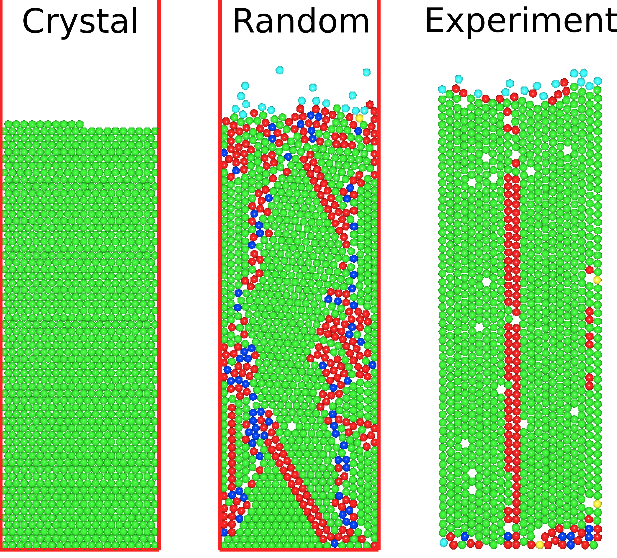
Figure 1: (colour online) Simulation snapshots of the typical initial configurations for $N_{l}=60$. The colour indicate the local order of the particles according to an analysis with the $q_{6}$ order parameter Steinhardt et al. (1983). Green (light grey) indicates hexagonal order, red (dark grey) indicates a square local order while other colours indicate a disordered configuration. From left to right: the crystalline and random initialisations of the simulation, and the experimental initial configuration.

The resulting configurations are shown in Fig. 1. We note that in both simulations initialised randomly and the experiments a large amount of particles have local hexagonal order with many topological defects, such as dislocations and grain boundaries. For a two dimensional system there are two favoured orientations of the hexagonal lattice, when in contact with a flat wall. In Fig. 2a) the Orientation A with the [111] direction parallel to the wall is shown. In Fig. 2b) the orientation B has the [010] direction parallel to the wall.

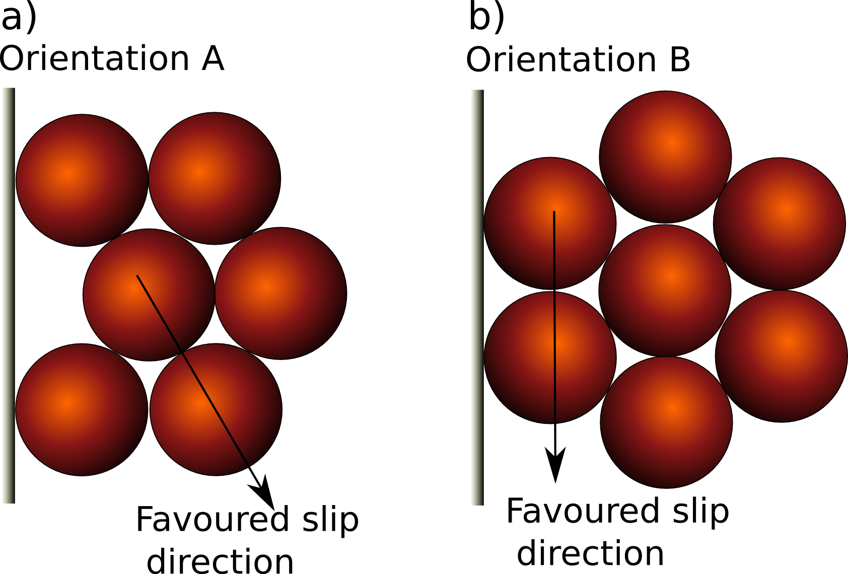
Figure 2: (colour online) Sketch of the possible orientations of the hexagonal crystal in contact with the lateral wall of the container box.

In the crystalline initialisation we chose to place the particles according to orientation A. After the random initialisation processes, we find that in the experiment almost all particles have orientation B, while in simulation the orientation A seems to be favoured, but grain boundaries between the different orientations are visible. Figure 1 shows the configurations obtained in the three cases.

IV Dynamical phases

We have systematically investigated the onset of convection at different dimensionless accelerations/energies and heights of the granular bed. Figure 3 shows the location of the dynamical phases as a function of the dimensionless acceleration $\Gamma$ and the energy parameter $K_{m}$ for different values of the linear density $N_{l}$. The parameter $N_{l}\sigma$ is also a measure of the number of layers in the granular bed, and therefore of its height.

The transition from the comoving to bouncing bed phase occurs, as expected, at $\Gamma$ slightly larger than one, with the critical value of the acceleration increasing slightly with increasing number of layers. We find good agreement between simulations (green triangles/blue circles) and experiments (connected squares). In experiments, the determination of this boundary is sensitive to the accuracy of the particle position determination, which is set by the resolution of the camera.

Inside the bouncing bed regime, we observe a transition from a bouncing bed phase without convection to a bouncing bed phase with convection. We find reasonable agreement between experiments and the simulations initialised randomly. For $N_{l}\sigma$=60,80 the model underestimates the amount of energy necessary for the convection to start. The discrepancy is probably related to variability in the concentration of defects, as well as to the presence of the front and back wall in the experiments. For simulations that start without topological defects we consistently detect the onset of convection (blue circles) at higher values of the acceleration with respect to the experiments and to the simulations started with defects. The enhancement of the convection due to the presence of defects explains the observation of Pöschel and Herrmann (1995) that an intruder can initiate convection. The presence of an intruder induces topological defects de Villeneuve et al. (2005) that initiate the convection and segregation.

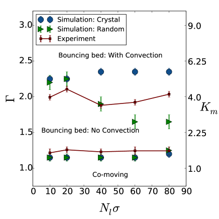
Figure 3: (colour online) Dynamical phases at different accelerations $\Gamma$ and linear density/number of layers $N_{l}\sigma$. On the right $y$-axis the energy parameter $K_{m}$ is also reported. Symbols are for simulation results for either the system initialised randomly (triangles) or in a crystalline configuration (circles). The connected squares are the experimental results.

V Onset of convection

In crystalline materials collective particle movements occur via crystalline plane slips Cooke et al. (1996). The same occurs in our granular systems, but we noted some differences in slip behaviour between simulation and experiments. In simulation the slip occur primarily along the oblique directions, while in the experiment it occurs mainly along the vertical direction. The difference can be explained by the different orientation of the hexagonal crystal in the two cases. The granular particles experience a shear stress due to the wall of the container along the vertical direction. In the experiments the particles are oriented like in Fig. 2b), and slips occur preferentially in the vertical direction. On the other hand, in simulations we find more particles with an orientation like in Fig. 2a) and the pyramidal slip planes will be activated first. As long as plane slips are concerned, the worst case scenario is represented by a perfect crystal with orientation A. Since no defects are initially present, slips along the pyramidal planes can only occur if defects are nucleated first. Another difference is that in experiments we often observe single convective rolls similar to the observation in a two-dimensional rotating cell Rietz and Stannarius (2012). This type of convective motion is not detected in simulation and the reason for the discrepancy is likely due to a small tilt of the side walls Knight et al. (1993).

In order to clarify the role of defects in the onset of convection, we analyse in computer simulations the granular temperature $T_{g}$ in relation to the average input energy $K_{m}$ The granular temperature is defined as

$$T_{g}=\frac{m}{N}\langle\sum_{i=1}^{N}\frac{1}{2}(\bm{v}_{i}(t)-\bm{v}_{\rm cm}(t))^{2}\rangle\,$$ (2)

where $\bm{v}_{\rm cm}$ is the centre of mass velocity and $\bm{v}_{i}(t)$ is the velocity of particle $i$ at time $t$ and $\langle\rangle$ indicates a time average. Figures 4a-b show the behaviour of the reduced granular temperature $T_{g}^{*}=T_{g}/(mg\sigma)$ as a function of the dimensionless energy parameter $K_{m}$ for systems initialised with and without defects, respectively. In both cases the temperature increases monotonically over many orders of magnitude. The curve gives an indication of how much input energy $K_{m}$ is converted into the kinetic energy of the granular particles.

We divide the energy $K_{m}$ parameter space in regions with different slopes of the temperature curves. For the random initialisation (Fig. 4a) we find two regions: $A$ and $B$. The transition occurs at $K_{m}\simeq 3.3$ as signalled by a change in slope of the temperature curve. Comparing the energy value for this transition with the diagram of Fig. 3, we note that it corresponds to the energy value at the onset of convection.

On the other hand, for the case initialised without defects (Fig. 4b) we can distinguish three regions. Following the naming convention used in Fig. 4a, we indicate with $B$ the region where convection is detected. The region $A$, without convection, is now divided in two subregions $A_{1}$ and $A_{2}$.

In order to clarify the origin of the different regions of temperature behaviour, we investigate the slip probability of a particle in the bulk of the granular bed, i.e. away from the top free interface . The slip of a particle is detected if a displacement larger than $0.2\leavevmode\nobreak\ \sigma$ is measured for at least two nearest neighbours after one oscillation. We define the slip probability $p_{s}$ as the fraction of particles which undergo a slip in one oscillation period. The value of $p_{s}$ is averaged over 200 periods of oscillation. The slip probability as a function of $1/K_{m}$ is shown in Figs. 5a-b for the random and crystal initialisation, respectively. For the random case we do not observe a change in the slip behaviour between regions $A$ and $B$. On the other hand a quite dramatic change of behaviour is observed for the crystal case. In particular, in region $A_{1}$ the number of detected slip is exactly zero, while region $A_{2}$ is characterised by a quite steep increase of slip events, which slows down considerably upon onset of convection (region $B$).

In all cases the curves can be fitted to an Arrhenius law, $p_{s}\propto\exp(-E_{b}/K_{m})$, indicating the presence of activating mechanisms. The energy parameter $E_{b}$ is a measure of the barrier height and the dimensionless energy $K_{m}$ assumes the role of a reservoir temperature. For the random case just a single curve can be fitted to the entire range of inverse energies. From the fit we find an average dimensionless barrier height $E_{b}=7\pm 1$. For the case initialised with the crystal, we find a barrier $E_{b}=130\pm 20$ in region $A_{2}$, and a barrier $E_{b}=7\pm 1$ in region $B$.

Since the barrier height is the same for the system with initial defects, independent of the presence of convection, we can speculate that the activation mechanism indicated by the Arrhenius equation is the activation of slip events in a crystal with topological defects. Interestingly, the same barrier is measured for the system without initial defects in region B, suggesting the same activation mechanism. But in order for this to occur defects must first nucleate inside a perfect crystal, and we speculate that the very high barrier in region $A_{2}$ is due to the nucleation of defects in a perfect hexagonal crystal.

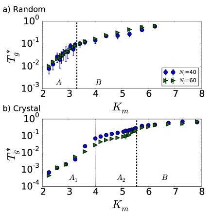
Figure 4: (colour online) Granular temperature $T_{g}$ versus dimensionless energy parameter $K_{m}$. The dashed lines separate regions with different slopes of the temperature curves. a) For the system initialised randomly, i.e. with defects. b) For the system initialised in a perfect hexagonal lattice, i.e. without initial defects.

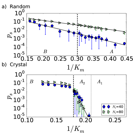
Figure 5: (colour online) Slip probability $p_{s}$ versus the inverse dimensionless energy parameter $1/K_{m}$. The continuos lines represent exponential fit functions. The dashed lines separate the regions defined in Fig. 4. a) For the system initialised randomly, i.e. with defects. b) For the system initialised in a perfect hexagonal lattice, i.e. without initial defects.

VI Conclusions

In conclusion, using two-dimensional computer simulations and experiments we locate the wall-induced convection in the bouncing bed region in the dynamical phase diagram of vertically vibrated granular matter.

For the onset of convection, we find a reasonable agreement between the experimental results and those from simulations initialised with defects. We believe the reason behind the discrepancy is the presence of a front and a back wall in the experimental box, as well as some variability, due to the presence of defects. Other phenomenological differences between simulations and experiments are observed for the favoured crystal orientation and slip events. We think that these differences are due to a small tilt of the experimental box and small variations of the experimental box width $L_{x}$.

For a system initialised in a perfect crystal, i.e., without initial defects, we consistently observe the wall-induced convective motion to occur at higher values of the dimensionless energy parameter (shaking strength) with respect to the system initialised randomly. From the analysis of the granular temperature we distinguish different regions based on the slope of the temperature as a function of the dimensionless energy $K_{m}$. For systems initialised randomly, i.e. with many initial defects, we distinguish two regions ($A$ and $B$) of temperature. The transition between the two regions occurs at the onset of convection, but we do not observe any change in the slip probability in the transition between regions $A$ and $B$.

On the other hand, for systems initialised with a perfect hexagonal lattice, i.e. without initial defects, we distinguish three regions in the temperature curve. Moreover, in this case the slip probability has very different behaviour in the three regions. In particular, in region $A_{1}$ the number of detected slips is exactly zero, while region $A_{2}$ is characterised by a quite steep increase of slip events with the input energy, which slows down considerably upon onset of convection (region $B$).

The slip probability follows an Arrhenius law, indicating the presence of an activating mechanisms. The very high barrier in the region $A_{2}$ of the system without defects is due to the nucleation of defects in the perfect hexagonal crystal. We noted that the barrier in region $B$ is the same for the system initialised with and without initial defects. In this region the behaviour of the slip probability is related to the activation of slip events.

The results of our work provide an explanation for the onset of the convective regime in vertically oscillated granular systems and show that defects enhance onset of convection, i.e. systems with topological defects show convection at lower oscillation strengths, with respect to systems without defects. More work is needed to quantify the degree of variability for the onset of convection due to its sensitivity to the concentration and possibly types of defects. Interestingly, since defects can diffuse out of the system when they reach the top of the granular bed, regions of transient convective motion are possible, provided that the time scale for the defects diffusion is larger than the time scale for the nucleation of defects. This conjecture was not studied in this work, but represents an interesting avenue of future research. Furthermore, we plan to study how the size polydispersity of the granular particles changes the onset of the wall-induced convection as well as the influence of the box size on the dynamical behaviour. Furthermore, we would like to explore the effect of shock waves Huang et al. (2006) on the dynamical behaviour of the system.

Appendix A Details of the Model

We carry out Molecular Dynamics simulations at fixed time step $dt$, for two translational degrees of freedom and one rotational degree of freedom for a system of soft disks. An illustration of the model is shown in Fig. 6. Two particles at positions $\bm{r}_{i}$ and $\bm{r}_{j}$ with velocities $\bm{v}_{i}$ and $\bm{v}_{j}$ and angular velocities $\bm{\omega}_{i}$ and $\bm{\omega}_{j}$ define a system with an effective mass $m_{\rm eff}=m_{i}m_{j}/(m_{i}+m_{j})$ and a normal unit vector $\bm{n}_{ij}=\frac{\bm{r}_{i}-\bm{r}_{j}}{|\bm{r}_{i}-\bm{r}_{j}|}$. The tangential direction is defined as $\bm{t}_{ij}=\frac{\bm{v}_{t_{ij}}}{|\bm{v}_{t_{ij}}|}$ where

$$\bm{v}_{t_{ij}}=\bm{v}_{ij}-\bm{v}_{n_{ij}}-\frac{1}{2}(\sigma_{i}\bm{\omega}_{i}+\sigma_{j}\bm{\omega}_{j})\times\bm{n}_{ij}\ ,$$ (3)

with $\bm{v}_{n_{ij}}=(\bm{v}_{ij}\cdot\bm{n}_{ij})\bm{n}_{ij}$.

We define the displacement in the two directions $\delta_{n_{ij}}=d-|\bm{r}_{i}-\bm{r}_{j}|$, with $d=1/2(\sigma_{i}+\sigma_{j})$, and $\delta_{t_{ij}}\bm{t}_{ij}=\bm{v}_{t_{ij}}dt$. For the disk-disk interactions we use a linear model with forces

$$\bm{F}_{n_{ij}} = (\kappa_{n}\delta_{n_{ij}}\bm{n}_{ij}-\gamma_{n}m_{eff}\bm{v}_{n_{ij}})$$ (4)

$$\bm{F}_{t_{ij}} = (-\kappa_{t}\delta_{t_{ij}}\bm{t}_{ij}-\gamma_{t}m_{eff}\bm{v}_{t_{ij}})\ ,$$ (5)

in the normal and shear tangential directions, respectively. The parameters $\kappa_{n}$ and $\kappa_{t}$ are the stiffness coefficients in the normal and tangential direction, respectively. The energy dissipated during the contact is regulated by the damping coefficients $\gamma_{n}$ and $\gamma_{t}$. In addition we model the static friction by keeping track of the elastic shear displacement $\delta_{t_{ij}}$ over the contact lifetime and truncate it such that the Coulomb condition $|F_{t_{ij}}|<|\mu F_{n_{ij}}|$ is satisfied, where $\mu$ is the static friction coefficient.

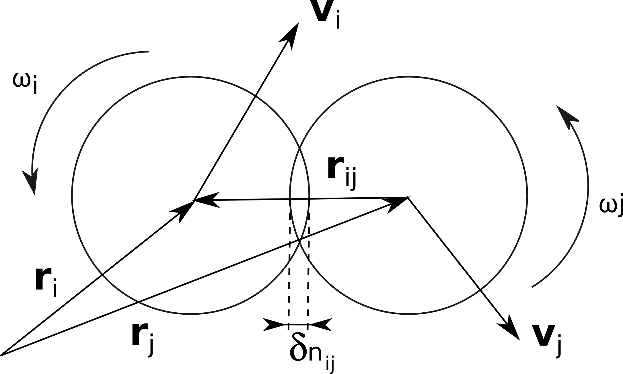
Figure 6: Illustration of the contact model of two granular disks at distance $\bm{r}_{ij}=\bm{r}_{i}-\bm{r}_{j}$ and relative velocity $\bm{v}_{ij}=\bm{v}_{i}-\bm{v}_{j}$, which overlap by a distance $\delta_{n_{ij}}$.

The same kind of interaction is used between the particles and the container wall. We also consider the gravitational force $\bm{g}=-g\bm{e_{z}}$, where $\bm{e_{z}}$ is the unit vector pointing in $z$ direction.

Once the forces on all particles are known the total force and torque $\tau_{i}$ on a particle $i$ is determined by

$$\bm{F}_{i} = m\bm{g}+\sum_{j}(\bm{F}_{n_{ij}}+\bm{F}_{t_{ij}})$$ (6)

$$\bm{\tau}_{i} = -\frac{1}{2}\sum_{j}\sigma_{j}\bm{n}_{ij}\times\bm{F}_{t_{ij}}\ .$$

Coefficient		Particle-Particle	Wall-Particle
Normal stiffness	$k_{n}$	$10^{6}\leavevmode\nobreak\ (k_{0})$	$10^{6}\leavevmode\nobreak\ (k_{0})$
Tangential stiffness	$k_{t}$	$10^{4}\leavevmode\nobreak\ (k_{0})$	$10^{4}\leavevmode\nobreak\ (k_{0})$
Static friction	$\mu$	0.6	0.6
Normal damping	$\gamma_{n}$	100 ($\gamma_{0})$	100 ($\gamma_{0})$
Tangential damping	$\gamma_{t}$	100 ($\gamma_{0})$	100 ($\gamma_{0})$

Table 1: Numerical values of the simulation parameters.

The typical numerical values of simulation parameters are shown in Table 1. In this linear model it is possible to calculate the contact duration Schäfer et al. (1996)

$$t_{c}=\pi\left(\frac{k_{n}}{m_{eff}}-\frac{\gamma_{n}^{2}}{4}\right)^{-0.5}\ .$$ (7)

In order to obtain an accurate integration of the equation of motion during contact, the time step of the simulation is chosen to be $\delta t\approx t_{c}/50$ Lee (1994).

Appendix B Detection of the dynamical phases

The detection of the convective motion, in both computer simulations and experiments, is performed by using $N_{t}$ tracer particles, which are initially positioned at the centre of the oscillating box in a straight horizontal line. In order to determine the threshold for convection, we analyse the deviation of the imaginary line connecting the tracer particles from the initial straight horizontal configuration. This is carried out by calculating, at the beginning of each cycle, the variance the tracers height from their average height

$$s^{2}_{j}=\frac{1}{N_{t}}\sum_{i=1}^{N_{t}}\left(z^{i}_{j}-\langle z_{j}\rangle\right)^{2}\ ,$$ (8)

where $\langle z_{j}\rangle$ is the average vertical position of the tracers at frame $j$ and $z^{i}_{j}$ is the vertical position of tracer $i$ at the beginning of cycle $j$.

An average variance over all $N_{f}$ frames is calculated

$$s^{2}_{\rm c}=\frac{1}{N_{f}}\sum_{j=1}^{N_{f}}s^{2}_{j}\ ,$$ (9)

and the start of the convection is identified via the condition $s_{\rm c}>\sigma$, where $\sigma$ is the diameter of the grains.

The detection of the bouncing bed dynamical phase is performed by detecting the detachment of the granular bed from the bottom plate, which can occur at any phase of the oscillating cycle. Therefore, we calculate the average height of the tracers with respect to the oscillating plate for each phase $k$

$$s(k)=\frac{1}{N_{f}}\sum_{j=1}^{N_{f}}(\langle z_{j}(k)\rangle_{i}-z_{\rm b}(k)),$$ (10)

where $\langle z_{j}(k)\rangle_{i}=\frac{1}{N_{t}}\sum_{i=1}^{N_{t}}z_{j}^{i}(k)$ is the average height of all $N_{t}$ tracer particles at phase $k$ and cycle $j$, $z_{\rm b}(k)$ is the height of the plate at phase $k$, and $N_{f}$ is the total number of frames at a certain phase.

Consequently, the variance over all $N_{k}$ phases is calculated

$$s^{2}_{\rm b}=\frac{1}{N_{k}}\sum_{k=1}^{N_{k}}s^{2}(k),$$ (11)

and the bouncing bed phase is identified with the condition $s_{\rm b}>\sigma/30$. The value $\sigma/30$ corresponds to half a pixel of the experimental images. For the sake of comparison, the same value is used in the analysis of the simulation trajectories.